

Item Difficulty Prediction Using Item Text Features: Comparison of Predictive Performance across Machine-Learning Algorithms

Abstract
:1. Introduction
2. Materials and Methods
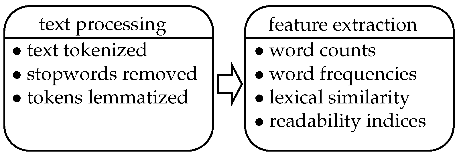
2.1. Dataset and Item Text Processing
2.2. Item Difficulty Based on Student Responses
2.3. Machine Learning Algorithms
2.3.1. Regularization
2.3.2. Naïve Bayes Classifier
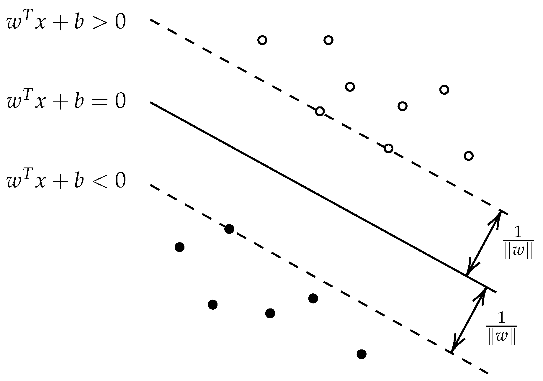
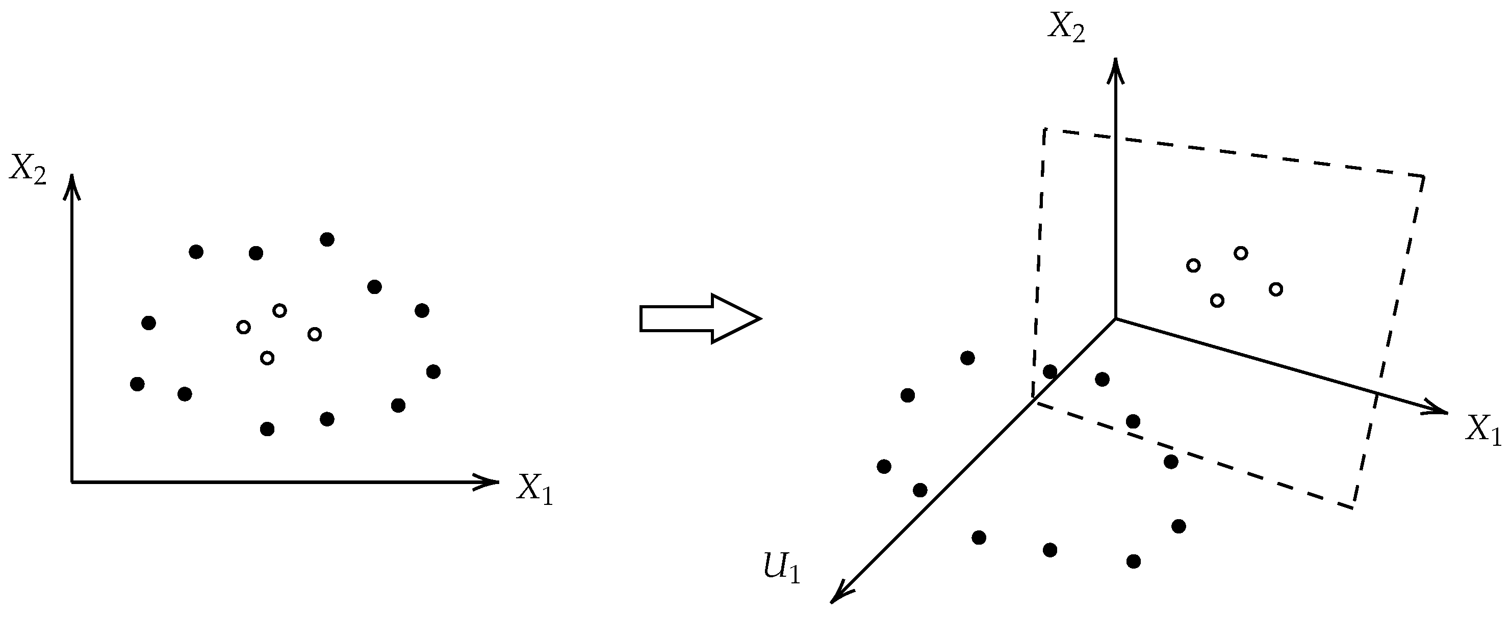
2.3.3. Support Vector Machines
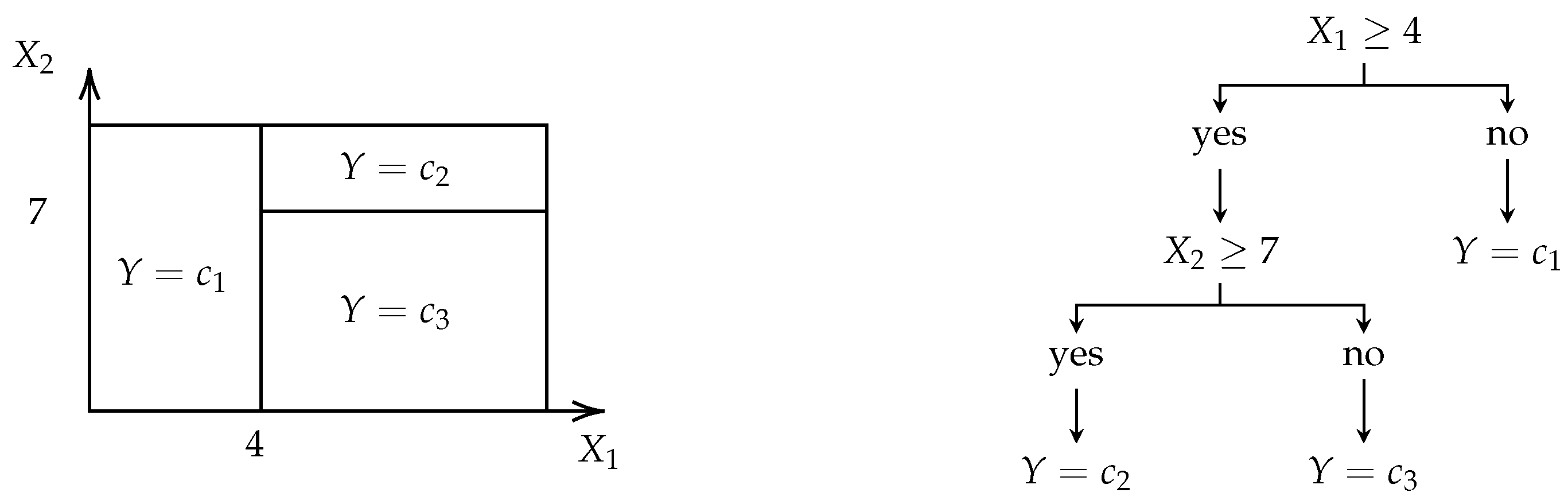
2.3.4. Regression and Classification Trees and Random Forests
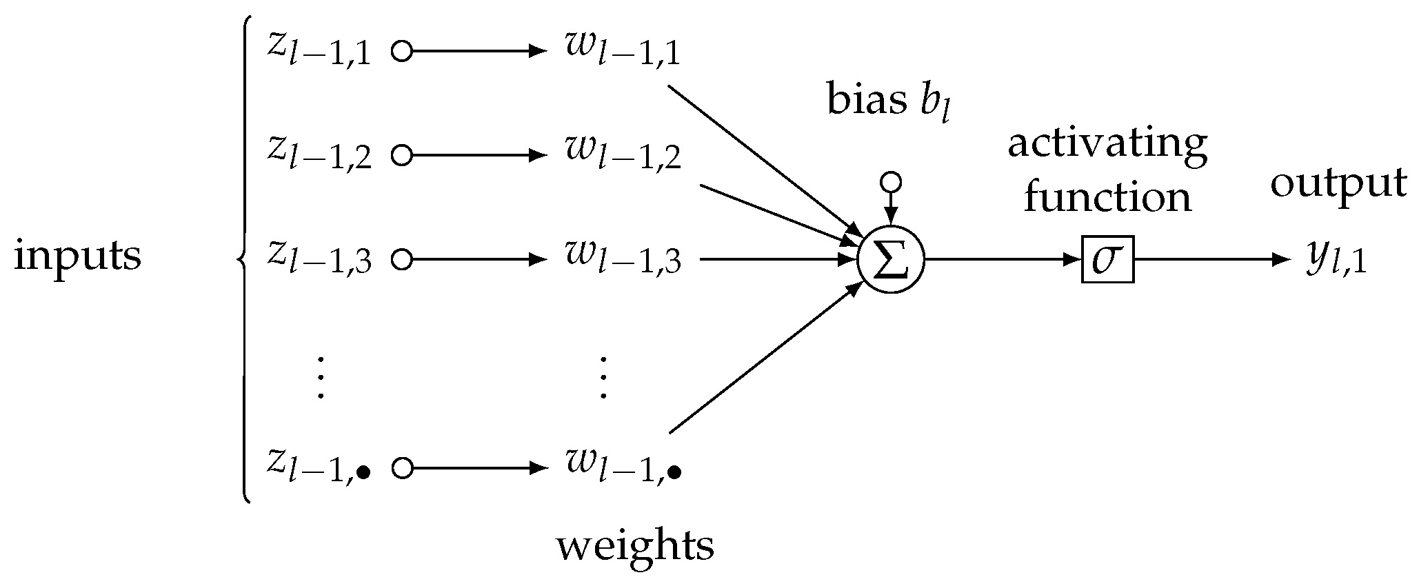
2.3.5. Neural Networks
2.3.6. Variable Importance Analysis
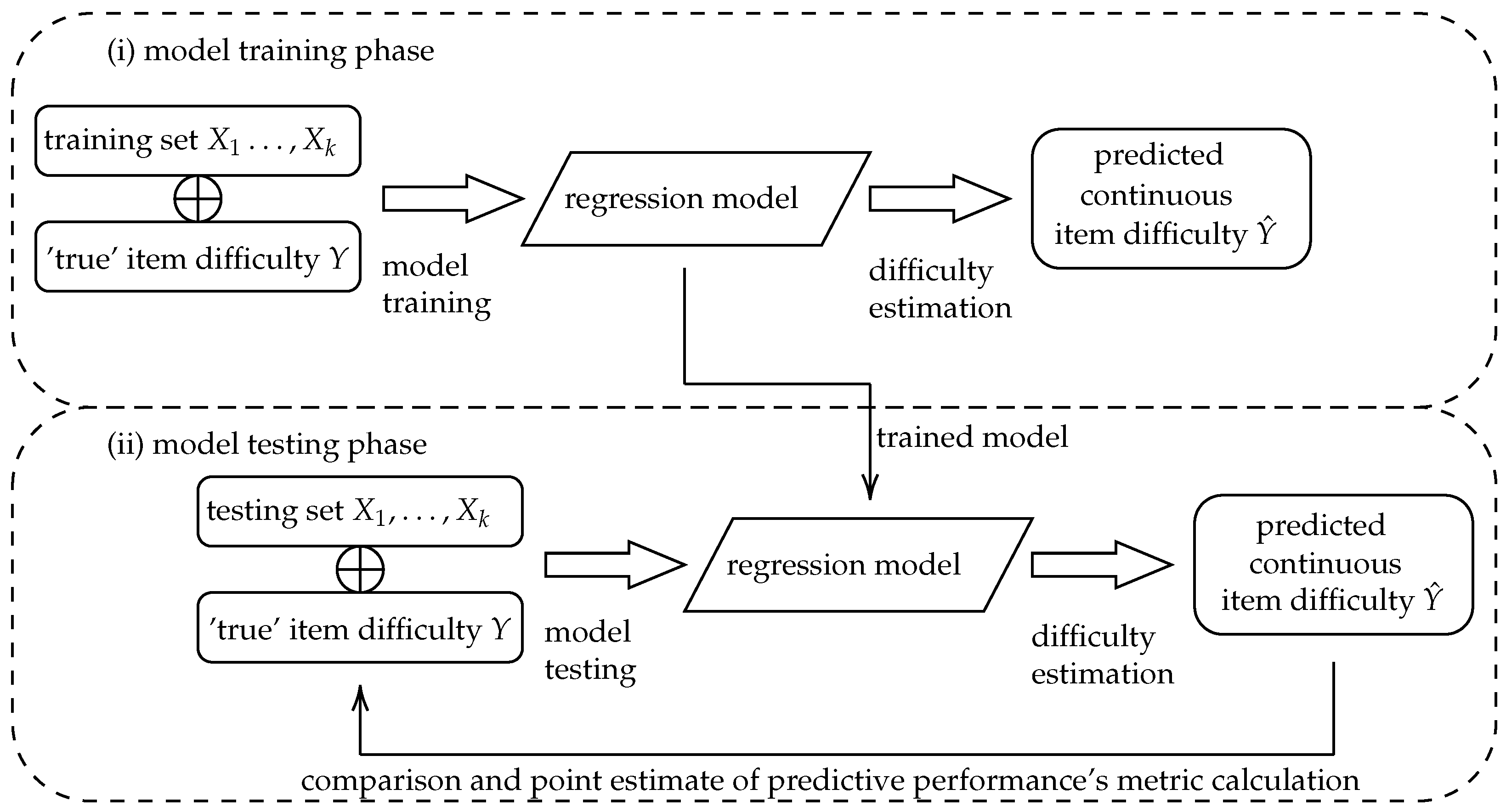
2.4. Evaluation of Algorithm Performance
2.4.1. Evaluation of Regression Performance
2.4.2. Evaluation of Classification Performance
2.4.3. Cross-Validation
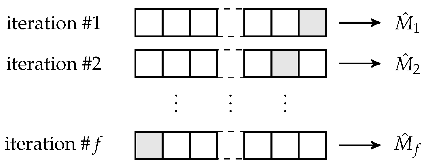
2.4.4. Relationship between Model’s Predictive Performance and a Number of Item Features in a Model
3. Implementation
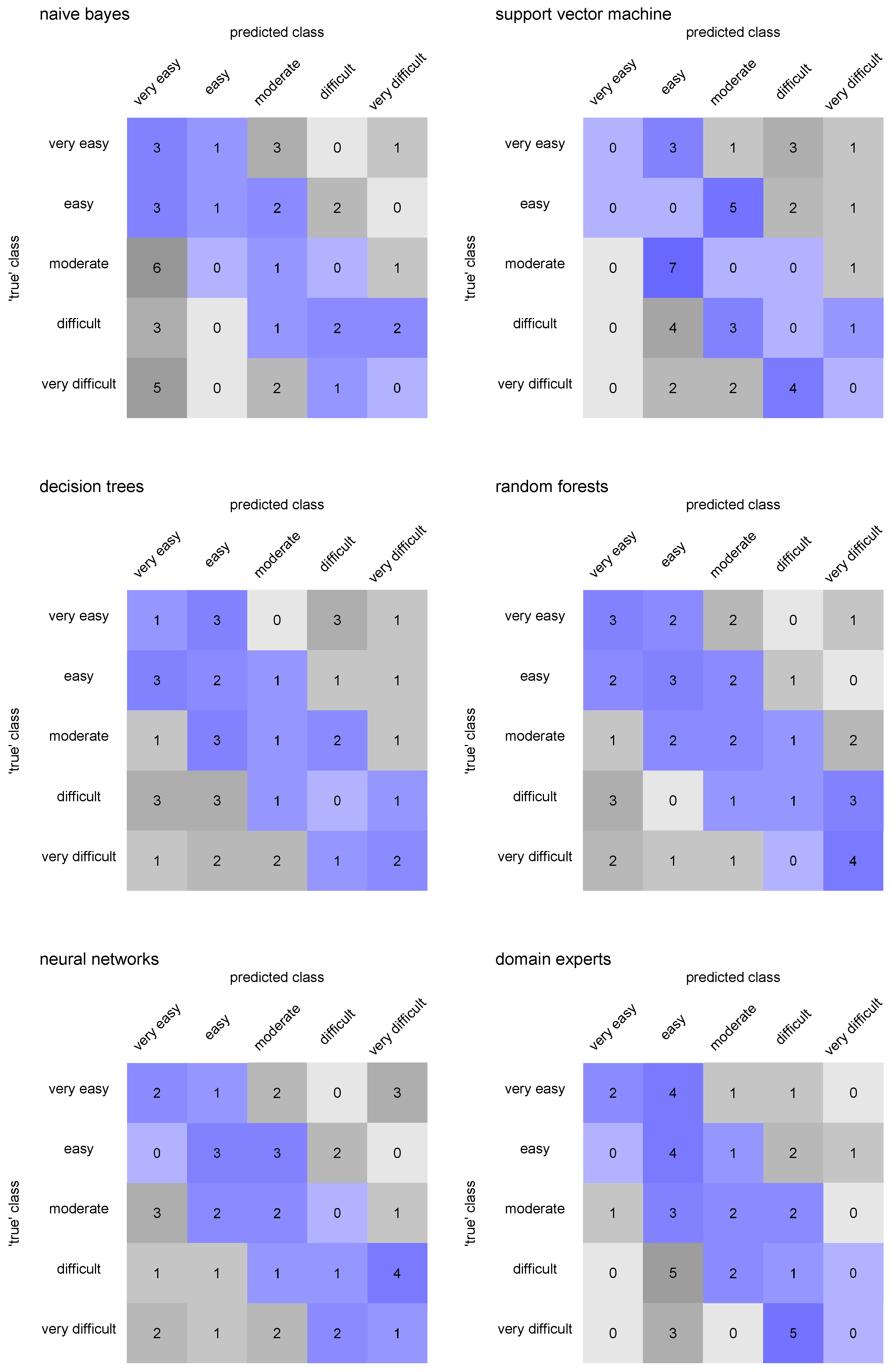
4. Results
5. Discussion
6. Conclusions
Author Contributions
Funding
Data Availability Statement
Acknowledgments
Conflicts of Interest
Appendix A
| Item Feature | Description or Definition of the Item Feature |
| number of characters | Total number of characters in a text of the item wording. |
| {}–number of characters | Total number of characters in a text of part of the item wording. |
| number of tokens | Total number of unique tokens, i.e., words in a text of the item wording. |
| {}–number of tokens | Total number of unique tokens, i.e., words in a text of part of the item wording. |
| number of monosyllabic words | Number of monosyllabic words, i.e., words with only one syllable in a text of the item wording. |
| {}–number of monosyllabic words | Number of monosyllabic words, i.e., words with only one syllable in a text of part of the item wording. |
| number of multi-syllable words | Number of multi-syllable words, i.e., words with more than three syllables in a text of the item wording. |
| {}–number of multi-syllable words | Number of multi-syllable words, i.e., words with more than three syllables in a text of part of the item wording. |
| average word length (characters) | Average number of characters in words in a text of the item wording. |
| {}–average word length (characters) | Average number of characters in words in a text of part of the item wording. |
| longest word length (characters) | Number of characters contained by the longest word in a text of the item wording. |
| {}–longest word length (characters) | Number of characters contained by the longest word in a text of part of the item wording. |
| average sentence length (words) | Average number of words in sentences in a text of the item wording. |
| {}–average sentence length (words) | Average number of words in sentences in a text of part of the item wording. |
| word length’s standard deviation (characters) | Standard deviation of a number of characters in words in a text of the item wording. |
| {}–word length’s standard deviation (characters) | Standard deviation of a number of characters in words in a text of part of the item wording. |
| number of uncommon words, according to COCA corpus | Number of words in a text of the item wording that appear uncommonly as defined in COCA (Corpus of Contemporary American English) corpus. |
| number of rare words, according to COCA corpus | Number of words in a text of the item wording that appear rarely as defined in COCA (Corpus of Contemporary American English) corpus. |
| frequency of the A1 words (CEFR) | Frequency of words in a text of the item wording at A1 level in CEFR (Common European Framework of Reference for Languages) scale. |
| frequency of the B2–C2 words (CEFR) | Frequency of words in a text of the item wording at B2–C2 levels in CEFR (Common European Framework of Reference for Languages) scale. |
| number of footnotes (hints) in the item | Total number of footnotes or hints in a text of the item wording. |
| Dale-Chall index | The readability score of a text of the item wording based on Dale-Chall readability formula. Dale-Chall readability formula follows,
|
| FOG index | The readability score of a text of the item wording based on Gunning’s Fog Index. The formula is
|
| SMOG index | The readability score of a text of the item wording based on Simple Measure of Gobbledygook (SMOG) index, so
|
| Traenkle-Bailer index | The readability score of a text of the item wording based on Traenkle-Bailer index (mostly used in German-speaking countries) is calculated as
|
| –euclidean distance | Let us assume two textual parts of item wording, and , so that a union of their tokens has a length . Additionally, let us assume two vectors of the same length l, i.e., and , where (or ) if and only if text (text ) contains token i, otherwise is (or ), for . The euclidean distance between the parts and is
|
| –cosine similarity | Again, let us assume two textual parts of item wording, and , so that a union of their tokens has a length . Additionally, let us assume two vectors of the same length l, i.e., and , where (or ) if and only if text (text ) contains token i, otherwise is (or ), for . The cosine similarity between the parts and is
|
| –word2vec similarity | Similarity of parts and of the item wording based on word2vec algorithms. Vectors of tokens for each part and are generated, and the similarity between them is captured from the context [88]. Thus, text parts with similar context end up with similar vectors and high word2vec similarity. |
| –common words1 | Proportion of common words from a text of part found in a text of part of the item wording. Let us assume two textual parts of item wording, and , so that a union of their tokens, called also document-feature matrix
has a length . Additionally, let us assume two vectors of the same length l, i.e., and , where (or ) if and only if text (text ) contains token i, otherwise is (or ), for . Then the –common words1 is
|
| –common words2 | Proportion of common words from a text of part found in a text of part of the item wording. Let us assume two textual parts of item wording, and , so that a union of their tokens, called also document-feature matrix
has a length . Additionally, let us assume two vectors of the same length l, i.e., and , where (or ) if and only if text (text ) contains token i, otherwise is (or ), for . Then the –common words2 is
|
| –number of features from a document-feature (DF) matrix | Let us assume two textual parts of item wording, and , so that a union of their tokens, called also document-feature matrix
(abbreviated as DF matrix) has a length . Additionally, let us assume two vectors of the same length l, i.e., and , where (or ) if and only if text (text ) contains token i, otherwise is (or ), for . The number of features from a document-feature matrix for the parts and is equal to
|
References
- Martinková, P.; Hladká, A. Computational Aspects of Psychometric Methods: With R; CRC Press: Boca Raton, FL, USA, 2023. [Google Scholar] [CrossRef]
- Kumar, V.; Boulanger, D. Explainable Automated Essay Scoring: Deep Learning Really Has Pedagogical Value. Front. Educ. 2020, 5, 572367. [Google Scholar] [CrossRef]
- Amorim, E.; Cançado, M.; Veloso, A. Automated Essay Scoring in the Presence of Biased Ratings. In Proceedings of the 2018 Conference of the North American Chapter of the Association for Computational Linguistics: Human Language Technologies, New Orleans, LA, USA, 1–6 June 2018; Association for Computational Linguistics: New Orleans, LA, USA, 2018. 1 (Long Papers). pp. 229–237. [Google Scholar] [CrossRef]
- Tashu, T.M.; Maurya, C.K.; Horvath, T. Deep Learning Architecture for Automatic Essay Scoring. arXiv 2022, arXiv:2206.08232. [Google Scholar] [CrossRef]
- Flor, M.; Hao, J. Text Mining and Automated Scoring; Springer International Publishing: Cham, Switzerland, 2021; pp. 245–262. [Google Scholar] [CrossRef]
- Attali, Y.; Runge, A.; LaFlair, G.T.; Yancey, K.; Goodwin, S.; Park, Y.; Davier, A.A.v. The interactive reading task: Transformer-based automatic item generation. Front. Artif. Intell. 2022, 5, 903077. [Google Scholar] [CrossRef]
- Gierl, M.J.; Lai, H.; Turner, S.R. Using automatic item generation to create multiple-choice test items. Med. Educ. 2012, 46, 757–765. [Google Scholar] [CrossRef]
- Du, X.; Shao, J.; Cardie, C. Learning to Ask: Neural Question Generation for Reading Comprehension. In Proceedings of the 55th Annual Meeting of the Association for Computational Linguistics (Volume 1: Long Papers), Vancouver, BC, Canada, 30 July–4 August 2017; Association for Computational Linguistics: Vancouver, Canada, 2017; pp. 1342–1352. [Google Scholar] [CrossRef]
- Settles, B.; T LaFlair, G.; Hagiwara, M. Machine learning–driven language assessment. Trans. Assoc. Comput. Linguist. 2020, 8, 247–263. [Google Scholar] [CrossRef]
- Kochmar, E.; Vu, D.D.; Belfer, R.; Gupta, V.; Serban, I.V.; Pineau, J. Automated Data-Driven Generation of Personalized Pedagogical Interventions in Intelligent Tutoring Systems. Int. J. Artif. Intell. Educ. 2022, 32, 323–349. [Google Scholar] [CrossRef]
- Gopalakrishnan, K.; Dhiyaneshwaran, N.; Yugesh, P. Online proctoring system using image processing and machine learning. Int. J. Health Sci. 2022, 6, 891–899. [Google Scholar] [CrossRef]
- Kaddoura, S.; Popescu, D.E.; Hemanth, J.D. A systematic review on machine learning models for online learning and examination systems. PeerJ Comput. Sci. 2022, 8, e986. [Google Scholar] [CrossRef]
- Kamalov, F.; Sulieman, H.; Santandreu Calonge, D. Machine learning based approach to exam cheating detection. PLoS ONE 2021, 16, e0254340. [Google Scholar] [CrossRef]
- von Davier, M.; Tyack, L.; Khorramdel, L. Scoring Graphical Responses in TIMSS 2019 Using Artificial Neural Networks. Educ. Psychol. Meas. 2023, 83, 556–585. [Google Scholar] [CrossRef]
- von Davier, M.; Tyack, L.; Khorramdel, L. Automated Scoring of Graphical Open-Ended Responses Using Artificial Neural Networks. arXiv 2022, arXiv:2201.01783. [Google Scholar] [CrossRef]
- von Davier, A.A.; Mislevy, R.J.; Hao, J. (Eds.) Computational Psychometrics: New Methodologies for a New Generation of Digital Learning and Assessment: With Examples in R and Python; Methodology of Educational Measurement and Assessment; Springer International Publishing: Cham, Switzerland, 2021. [Google Scholar] [CrossRef]
- Hvitfeldt, E.; Silge, J. Supervised Machine Learning for Text Analysis in R; Chapman and Hall/CRC: Boca Raton, FL, USA, 2021. [Google Scholar]
- Ferrara, S.; Steedle, J.T.; Frantz, R.S. Response demands of reading comprehension test items: A review of item difficulty modeling studies. Appl. Meas. Educ. 2022, 35, 237–253. [Google Scholar] [CrossRef]
- Belov, D.I. Predicting Item Characteristic Curve (ICC) Using a Softmax Classifier. In Proceedings of the Annual Meeting of the Psychometric Society; Springer: Cham, Switzerland, 2022; pp. 171–184. [Google Scholar] [CrossRef]
- AlKhuzaey, S.; Grasso, F.; Payne, T.R.; Tamma, V. A systematic review of data-driven approaches to item difficulty prediction. In Lecture Notes in Computer Science; Lecture notes in computer science; Springer International Publishing: Cham, Switzerland, 2021; pp. 29–41. [Google Scholar]
- James, G.; Witten, D.; Hastie, T.; Tibshirani, R. An Introduction to Statistical Learning; Springer: New York, NY, USA, 2021. [Google Scholar] [CrossRef]
- Jurafsky, D. Speech and Language Processing: An Introduction to Natural Language Processing, Computational Linguistics, and Speech Recognition; Pearson Prentice Hall: Upper Saddle River, NJ, USA, 2009. [Google Scholar]
- Chomsky, N. Three models for the description of language. IEEE Trans. Inf. Theory 1956, 2, 113–124. [Google Scholar] [CrossRef]
- Davies, M. The Corpus of Contemporary American English (COCA). 2008. Available online: http://corpus.byu.edu/coca/ (accessed on 29 June 2023).
- Davies, M. Most Frequent 100,000 Word Forms in English (Based on Data from the COCA Corpus). 2011. Available online: https://www.wordfrequency.info/ (accessed on 29 June 2023).
- Tonelli, S.; Tran Manh, K.; Pianta, E. Making Readability Indices Readable. In Proceedings of the First Workshop on Predicting and Improving Text Readability for Target Reader Populations; Association for Computational Linguistics: Montréal, QC, Canada, 2012; pp. 40–48. [Google Scholar]
- Rasch, G. Probabilistic Models for Some Intelligence and Attainment Tests; The University of Chicago Press: Chicago, IL, USA, 1993. [Google Scholar]
- Debelak, R.; Strobl, C.; Zeigenfuse, M.D. An introduction to the Rasch Model with Examples in R; CRC Press: Boca Raton, FL, USA, 2022. [Google Scholar]
- Alpaydin, E. Introduction to Machine Learning; MIT Press: Cambridge, MA, USA, 2010. [Google Scholar]
- Tibshirani, R. Regression Shrinkage and Selection Via the Lasso. J. R. Stat. Soc. Ser. (Methodol.) 1996, 58, 267–288. [Google Scholar] [CrossRef]
- Hoerl, A.E.; Kennard, R.W. Ridge Regression: Biased Estimation for Nonorthogonal Problems. Technometrics 1970, 12, 55–67. [Google Scholar] [CrossRef]
- Tuia, D.; Flamary, R.; Barlaud, M. To be or not to be convex? A study on regularization in hyperspectral image classification. In Proceedings of the 2015 IEEE International Geoscience and Remote Sensing Symposium (IGARSS), Milan, Italy, 26–31 July 2015; IEEE: Piscataway, NJ, USA, 2015. [Google Scholar] [CrossRef]
- Zou, H.; Hastie, T. Regularization and Variable Selection Via the Elastic Net. J. R. Stat. Soc. Ser. Stat. Methodol. 2005, 67, 301–320. [Google Scholar] [CrossRef]
- Fan, J.; Li, R. Comment: Feature Screening and Variable Selection via Iterative Ridge Regression. Technometrics 2020, 62, 434–437. [Google Scholar] [CrossRef]
- Friedman, N.; Geiger, D.; Goldszmidt, M. Bayesian Network Classifiers. Mach. Learn. 1997, 29, 131–163. [Google Scholar] [CrossRef]
- Cortes, C.; Vapnik, V. Support-vector networks. Mach. Learn. 1995, 20, 273–297. [Google Scholar] [CrossRef]
- Schölkopf, B. The Kernel Trick for Distances. In Proceedings of the 13th International Conference on Neural Information Processing Systems (NIPS’00), Hong Kong, China, 3–6 October 2006; MIT Press: Cambridge, MA, USA, 2000; pp. 283–289. [Google Scholar]
- Gray, N.A.B. Capturing knowledge through top-down induction of decision trees. IEEE Expert 1990, 5, 41–50. [Google Scholar] [CrossRef]
- Breslow, L.A.; Aha, D.W. Simplifying decision trees: A survey. Knowl. Eng. Rev. 1997, 12, 1–40. [Google Scholar] [CrossRef]
- Rutkowski, L.; Jaworski, M.; Pietruczuk, L.; Duda, P. The CART Decision Tree for Mining Data Streams. Inf. Sci. 2014, 266, 1–15. [Google Scholar] [CrossRef]
- Breiman, L. Classification and Regression Trees; Chapman & Hall: New York, NY, USA, 1993. [Google Scholar]
- McCulloch, W.S.; Pitts, W. A logical calculus of the ideas immanent in nervous activity. Bull. Math. Biophys. 1943, 5, 115–133. [Google Scholar] [CrossRef]
- Rojas, R. The Backpropagation Algorithm. In Neural Networks; Springer: Berlin/Heidelberg, Germany, 1996; pp. 149–182. [Google Scholar] [CrossRef]
- Mishra, M.; Srivastava, M. A view of Artificial Neural Network. In Proceedings of the 2014 International Conference on Advances in Engineering & Technology Research (ICAETR-2014), Unnao, Kanpur, India, 1–2 August 2014; IEEE: Piscataway, NJ, USA, 2014. [Google Scholar] [CrossRef]
- Hastie, T.; Tibshirani, R.; Friedman, J. The Elements of Statistical Learning; Springer: New York, NY, USA, 2009. [Google Scholar] [CrossRef]
- Altmann, A.; Toloşi, L.; Sander, O.; Lengauer, T. Permutation importance: A corrected feature importance measure. Bioinformatics 2010, 26, 1340–1347. [Google Scholar] [CrossRef] [PubMed]
- Powers, D.M.W. Evaluation: From precision, recall and F-measure to ROC, informedness, markedness and correlation. arXiv 2020, arXiv:2010.16061. [Google Scholar]
- Provost, F.J.; Fawcett, T.; Kohavi, R. The Case against Accuracy Estimation for Comparing Induction Algorithms. In Proceedings of the Fifteenth International Conference on Machine Learning (ICML ’98), Madison, WI, USA, 24–27 July 1998; Morgan Kaufmann Publishers Inc.: San Francisco, CA, USA, 1998; pp. 445–453. [Google Scholar]
- Moore, A.W.; Lee, M.S. Efficient algorithms for minimizing cross validation error. In Proceedings of the 11th International Conference on Machine Learning, New Brunswick, NJ, USA, 10–13 July 1994; Morgan Kaufmann: Burlington, MA, USA, 1994; pp. 190–198. [Google Scholar]
- Kohavi, R. A Study of Cross-Validation and Bootstrap for Accuracy Estimation and Model Selection. In Proceedings of the 14th International Joint Conference on Artificial Intelligence–Volume 2 (IJCAI’95), Montréal, QC, Canada, 20–25 August 1995; Morgan Kaufmann Publishers Inc.: San Francisco, CA, USA, 1995; pp. 1137–1143. [Google Scholar]
- R Core Team. R: A Language and Environment for Statistical Computing; R Core Team: Vienna, Austria, 2021. [Google Scholar]
- Mair, P.; Hatzinger, R.; Maier, M.J.; Rusch, T.; Debelak, R. eRm: Extended Rasch Modeling. 2021. Available online: https://cran.r-project.org/web/packages/eRm/index.html (accessed on 29 June 2023).
- Benoit, K.; Watanabe, K.; Wang, H.; Nulty, P.; Obeng, A.; Müller, S.; Matsuo, A. Quanteda: An R Package for the Quantitative Analysis of Textual Data. J. Open Source Softw. 2018, 3, 774. [Google Scholar] [CrossRef]
- Friedman, J.; Tibshirani, R.; Hastie, T. Regularization Paths for Generalized Linear Models via Coordinate Descent. J. Stat. Softw. 2010, 33, 1–22. [Google Scholar] [CrossRef]
- Meyer, D.; Dimitriadou, E.; Hornik, K.; Weingessel, A.; Leisch, F. e1071: Misc Functions of the Department of Statistics, Probability Theory Group (Formerly: E1071), TU Wien. 2023. R Package Version 1.7-13. Available online: https://rdrr.io/rforge/e1071/ (accessed on 29 June 2023).
- Therneau, T.; Atkinson, B. rpart: Recursive Partitioning and Regression Trees, 2022. R Package Version 4.1.19. Available online: https://cogns.northwestern.edu/cbmg/LiawAndWiener2002.pdf (accessed on 29 June 2023).
- Liaw, A.; Wiener, M. Classification and Regression by Random Forest. R News 2002, 2, 18–22. [Google Scholar]
- Fritsch, S.; Guenther, F.; Wright, M.N. neuralnet: Training of Neural Networks. 2019. R Package Version 1.44.2. Available online: https://journal.r-project.org/archive/2010/RJ-2010-006/RJ-2010-006.pdf (accessed on 29 June 2023).
- Craig, C.C. A Note on Sheppard’s Corrections. Ann. Math. Stat. 1941, 12, 339–345. [Google Scholar] [CrossRef]
- Chen, J.; de Hoogh, K.; Gulliver, J.; Hoffmann, B.; Hertel, O.; Ketzel, M.; Bauwelinck, M.; van Donkelaar, A.; Hvidtfeldt, U.A.; Katsouyanni, K.; et al. A comparison of linear regression, regularization, and machine learning algorithms to develop Europe-wide spatial models of fine particles and nitrogen dioxide. Environ. Int. 2019, 130, 104934. [Google Scholar] [CrossRef]
- Dong, Y.; Zhou, S.; Xing, L.; Chen, Y.; Ren, Z.; Dong, Y.; Zhang, X. Deep learning methods may not outperform other machine learning methods on analyzing genomic studies. Front. Genet. 2022, 13, 992070. [Google Scholar] [CrossRef]
- Su, J.; Fraser, N.J.; Gambardella, G.; Blott, M.; Durelli, G.; Thomas, D.B.; Leong, P.; Cheung, P.Y.K. Accuracy to Throughput Trade-offs for Reduced Precision Neural Networks on Reconfigurable Logic. arXiv 2018, arXiv:1807.10577. [Google Scholar] [CrossRef]
- Benedetto, L.; Cappelli, A.; Turrin, R.; Cremonesi, P. Introducing a Framework to Assess Newly Created Questions with Natural Language Processing. In Lecture Notes in Computer Science; Springer International Publishing: Cham, Switzerland, 2020; pp. 43–54. [Google Scholar] [CrossRef]
- Benedetto, L.; Cappelli, A.; Turrin, R.; Cremonesi, P. R2DE: A NLP approach to estimating IRT parameters of newly generated questions. In Proceedings of the Tenth International Conference on Learning Analytics & Knowledge; ACM: New York, NY, USA, 2020. [Google Scholar] [CrossRef]
- Ehara, Y. Building an English Vocabulary Knowledge Dataset of Japanese English-as-a-Second-Language Learners Using Crowdsourcing. In Proceedings of the Eleventh International Conference on Language Resources and Evaluation (LREC 2018), Miyazaki, Japan, 7–12 May 2018; European Language Resources Association (ELRA): Miyazaki, Japan, 2018. [Google Scholar]
- Lee, J.U.; Schwan, E.; Meyer, C.M. Manipulating the Difficulty of C-Tests. In Proceedings of the 57th Annual Meeting of the Association for Computational Linguistics, Florence, Italy, 28 July–2 August 2019; Association for Computational Linguistics: Florence, Italy, 2019; pp. 360–370. [Google Scholar] [CrossRef]
- Pandarova, I.; Schmidt, T.; Hartig, J.; Boubekki, A.; Jones, R.D.; Brefeld, U. Predicting the Difficulty of Exercise Items for Dynamic Difficulty Adaptation in Adaptive Language Tutoring. Int. J. Artif. Intell. Educ. 2019, 29, 342–367. [Google Scholar] [CrossRef]
- Qiu, Z.; Wu, X.; Fan, W. Question Difficulty Prediction for Multiple Choice Problems in Medical Exams. In Proceedings of the 28th ACM International Conference on Information and Knowledge Management, Beijing, China, 3–7 November 2019; ACM: New York, NY, USA, 2019. [Google Scholar] [CrossRef]
- Ha, L.A.; Yaneva, V.; Baldwin, P.; Mee, J. Predicting the Difficulty of Multiple Choice Questions in a High-stakes Medical Exam. In Proceedings of the Fourteenth Workshop on Innovative Use of NLP for Building Educational Applications, Florence, Italy, 2 August 2019; Association for Computational Linguistics: Florence, Italy, 2019; pp. 11–20. [Google Scholar] [CrossRef]
- Xue, K.; Yaneva, V.; Runyon, C.; Baldwin, P. Predicting the Difficulty and Response Time of Multiple Choice Questions Using Transfer Learning. In Proceedings of the Fifteenth Workshop on Innovative Use of NLP for Building Educational Applications, Online, 10 July 2020; Association for Computational Linguistics: Seattle, WA, USA, 2020; pp. 193–197. [Google Scholar] [CrossRef]
- Yaneva, V.; Ha, L.A.; Baldwin, P.; Mee, J. Predicting Item Survival for Multiple Choice Questions in a High-Stakes Medical Exam. In Proceedings of the Twelfth Language Resources and Evaluation Conference, Marseille, France, 11–16 May 2020; European Language Resources Association: Marseille, France, 2020; pp. 6812–6818. [Google Scholar]
- Yin, Y.; Liu, Q.; Huang, Z.; Chen, E.; Tong, W.; Wang, S.; Su, Y. QuesNet. In Proceedings of the 25th ACM SIGKDD International Conference on Knowledge Discovery & Data Mining, Anchorage, AK, USA, 4–8 August 2019; ACM: New York, NY, USA, 2019. [Google Scholar] [CrossRef]
- Hsu, F.Y.; Lee, H.M.; Chang, T.H.; Sung, Y.T. Automated estimation of item difficulty for multiple-choice tests: An application of word embedding techniques. Inf. Process. Manag. 2018, 54, 969–984. [Google Scholar] [CrossRef]
- Lin, L.H.; Chang, T.H.; Hsu, F.Y. Automated Prediction of Item Difficulty in Reading Comprehension Using Long Short-Term Memory. In Proceedings of the 2019 International Conference on Asian Language Processing (IALP), Shanghai, China, 15–17 November 2019; IEEE: Piscataway, NJ, USA, 2019. [Google Scholar] [CrossRef]
- McTavish, D.G.; Pirro, E.B. Contextual content analysis. Qual. Quant. 1990, 24, 245–265. [Google Scholar] [CrossRef]
- Stipak, B.; Hensler, C. Statistical Inference in Contextual Analysis. Am. J. Political Sci. 1982, 26, 151. [Google Scholar] [CrossRef]
- Martinková, P.; Štěpánek, L.; Drabinová, A.; Houdek, J.; Vejražka, M.; Štuka, Č. Semi-real-time analyses of item characteristics for medical school admission tests. In Proceedings of the 2017 Federated Conference on Computer Science and Information Systems, Prague, Czech Republic, 3–6 September 2017; IEEE: Piscataway, NJ, USA, 2017. [Google Scholar] [CrossRef]
- Erosheva, E.A.; Martinková, P.; Lee, C.J. When zero may not be zero: A cautionary note on the use of inter-rater reliability in evaluating grant peer review. J. R. Stat. Soc. Ser. (Stat. Soc.) 2021, 184, 904–919. [Google Scholar] [CrossRef]
- Van den Besselaar, P.; Sandström, U.; Schiffbaenker, H. Studying grant decision-making: A linguistic analysis of review reports. Scientometrics 2018, 117, 313–329. [Google Scholar] [CrossRef]
- Penfield, R.D.; Camilli, G. Differential item functioning and item bias. In Psychometrics; Rao, C.R., Sinharay, S., Eds.; Handbook of Statistics; Elsevier: Amsterdam, The Netherlands, 2006; Volume 26, pp. 125–167. [Google Scholar] [CrossRef]
- Martinková, P.; Drabinová, A.; Liaw, Y.L.; Sanders, E.A.; McFarland, J.L.; Price, R.M. Checking equity: Why differential item functioning analysis should be a routine part of developing conceptual assessments. CBE-Life Sci. Educ. 2017, 16, rm2. [Google Scholar] [CrossRef]
- Hladká, A.; Martinková, P. difNLR: Generalized Logistic Regression Models for DIF and DDF Detection. R J. 2020, 12, 300–323. [Google Scholar] [CrossRef]
- Martinková, P.; Hladká, A.; Potužníková, E. Is academic tracking related to gains in learning competence? Using propensity score matching and differential item change functioning analysis for better understanding of tracking implications. Learn. Instr. 2020, 66, 101286. [Google Scholar] [CrossRef]
- Chall, J.S.; Dale, E. Readability REVISITED: The New Dale-Chall Readability Formula; Brookline Books: Cambridge, MA, USA, 1995. [Google Scholar]
- Gunning, R. The Technique of Clear Writing; McGraw-Hill: New York, NY, USA, 1952. [Google Scholar]
- McLaughlin, G.H. SMOG Grading: A New Readability Formula. J. Read. 1969, 12, 639–646. [Google Scholar]
- Tränkle, U.; Bailer, H. Kreuzvalidierung und Neuberechnung von Lesbarkeitsformeln für die deutsche Sprache. Zeitschrift für Entwicklungspsychologie und Pädagogische Psychologie 1984, 16, 231–244. [Google Scholar]
- Mikolov, T.; Chen, K.; Corrado, G.; Dean, J. Efficient Estimation of Word Representations in Vector Space. arXiv 2013, arXiv:1301.3781. [Google Scholar]


| Predicted Class () | |||||
|---|---|---|---|---|---|
| ⋯ | |||||
| ‘true’ class () | ⋯ | ||||
| ⋯ | |||||
| ⋮ | ⋮ | ⋮ | ⋱ | ⋮ | |
| ⋯ | |||||
| Regression Algorithm | Root Mean Square Error (RMSE) |
|---|---|
| LASSO regression | 0.694 |
| Ridge regression | 0.719 |
| Elastic net regression | 0.666 |
| Support vector machines | 0.716 |
| Regression trees | 0.978 |
| Random forests | 0.719 |
| Neural networks | 0.971 |
| Domain experts | 1.004 |
| Classification Algorithm | Predictive Accuracy | Extended Predictive Accuracy |
|---|---|---|
| Naïve Bayes classifier | 0.175 | 0.425 |
| Support vector machines | 0.000 | 0.575 |
| Classification trees | 0.150 | 0.525 |
| Random forests | 0.325 | 0.650 |
| Neural networks | 0.225 | 0.550 |
| Domain experts | 0.225 | 0.650 |
| Item Feature | |
|---|---|
| Number of characters | 5.912 ± 0.673 |
| Word length’s standard deviation (characters) | |
| Passage and distractors–word2vec similarity | |
| Text readability–Traenkle-Bailer index | |
| Question and key item–word2vec similarity | |
| Distractors–average sentence length (words) | |
| Key option and distractors–number of features from a DF matrix | |
| Distractors–average word length (characters) | |
| Distractors–average word length (characters) | |
| Text readability–SMOG index | |
| Question and key option–number of features from a DF matrix | |
| Item passage and distractors–common words1 | |
| Passage and key option–word2vec similarity | |
| Text readability–FOG index | |
| Question and passage–euclidean distance | |
| Average word length (characters) | |
| Passage and key option–euclidean distance | |
| Passage and distractors–euclidean distance | |
| Item passage and distractors–cosine similarity | |
| Question and distractors–euclidean distance |
| Item Feature | |
|---|---|
| Word length’s standard deviation (characters) | |
| Number of characters | |
| Text readability–Traenkle-Bailer index | |
| Question and key item–word2vec similarity | |
| Passage and distractors–word2vec similarity | |
| Passage and distractors–euclidean distance | |
| Item passage and distractors–common words1 | |
| Distractors–average word length (characters) | |
| Distractors–average word length (characters) | |
| Question and passage–number of features from a DF matrix | |
| Text readability–FOG index | |
| Text readability–Dale-Chall index | |
| Text readability–SMOG index | |
| Distractors–average sentence length (words) | |
| Key option and distractors–number of features from a DF matrix | |
| Item passage and distractors–cosine similarity | |
| Average word length (characters) | |
| Question and passage–euclidean distance | |
| Average sentence length (words) | |
| Passage and key option–euclidean distance |
| Item Feature | Coefficient |
|---|---|
| (intercept) | −3.808 |
| Number of characters | 0.002 |
| Word length’s standard deviation (characters) | 0.809 |
| Distractors–average sentence length (words) | 0.002 |
| Dale-Chall index | 0.004 |
| FOG index | 0.026 |
| Passage and distractors–common words1 | 0.630 |
| Key option and distractors–word2vec similarity | 0.023 |
Disclaimer/Publisher’s Note: The statements, opinions and data contained in all publications are solely those of the individual author(s) and contributor(s) and not of MDPI and/or the editor(s). MDPI and/or the editor(s) disclaim responsibility for any injury to people or property resulting from any ideas, methods, instructions or products referred to in the content. |
© 2023 by the authors. Licensee MDPI, Basel, Switzerland. This article is an open access article distributed under the terms and conditions of the Creative Commons Attribution (CC BY) license (https://creativecommons.org/licenses/by/4.0/).
Share and Cite
Štěpánek, L.; Dlouhá, J.; Martinková, P. Item Difficulty Prediction Using Item Text Features: Comparison of Predictive Performance across Machine-Learning Algorithms. Mathematics 2023, 11, 4104. https://0-doi-org.brum.beds.ac.uk/10.3390/math11194104
Štěpánek L, Dlouhá J, Martinková P. Item Difficulty Prediction Using Item Text Features: Comparison of Predictive Performance across Machine-Learning Algorithms. Mathematics. 2023; 11(19):4104. https://0-doi-org.brum.beds.ac.uk/10.3390/math11194104
Chicago/Turabian StyleŠtěpánek, Lubomír, Jana Dlouhá, and Patrícia Martinková. 2023. "Item Difficulty Prediction Using Item Text Features: Comparison of Predictive Performance across Machine-Learning Algorithms" Mathematics 11, no. 19: 4104. https://0-doi-org.brum.beds.ac.uk/10.3390/math11194104