An Exact Approach for Selecting Pickup-Delivery Stations in Urban Areas to Reduce Distribution Emission Costs

Abstract

This paper deals with a variant of the multifacility location-routing problem in urban areas. The distribution network is modelled by an undirected graph, in which the nodes are split into a set of pickup-delivery stations, a depot, and a set of customers. The arcs represent the minimum-cost connections between nodes. A customer is assigned to a pickup-delivery station if he or she can reach it at the lowest sustainable cost, i.e., on foot or by bicycle, without exceeding a predefined maximum distance. The goal is to minimise the goods’ total delivery cost, including pollutant emissions. In this perspective, both travel distance and means of transport play a key role. We present an exact novel approach based on partitioning the research space of the solutions of a Mixed Integer Linear Programming model. In the model, Boolean decisional variables, representing the selection of the locations for the pickup-delivery stations, are fixed simultaneously with the solution of the classical Travelling Salesman Problem. A branching constraint allows us to determine the route that serves the selected pickup-delivery stations and the route, if any, that serves customers who do not go to any pickup-delivery station. We conduct extensive experimentation to test the proposed approach’s computational efficiency and analyse the optimal solution’s robustness with respect to the maximum distance of customers from the stations, their activation cost and the pollutant emissions. The effectiveness of the proposed approach in terms of solution quality and computation time is certified by a set of computational tests based on randomly generated instances with up to 150 customers and 30 pickup-delivery stations. The application of the proposed exact method to a case study related to a district of the city of Genoa (Italy) confirms its validity also for sustainably addressing real-size urban delivery problems. An evaluation of incentives for customers using pickup-delivery stations, possibly by implementing discount policies on orders, is also proposed.

1. Introduction and Problem Definition

Nowadays, there is a growing concern for climate change, especially in terms of the reduction of carbon emissions in urban and metropolitan areas. In this scenario, large retail business-to-consumer companies operating within cities are experiencing a period of great organisational change due to the need to supply customers in an increasingly environmentally sustainable manner (Cano et al., 2022 [1]).

As cost minimisation is one of the primary goals of distribution logistics, much attention in recent literature is focused on suggesting to interested companies how to limit delivery costs while minimising pollutant emissions (Dekker et al., 2012 [2]; Bektaş et al., 2019 [3]; Heshmati et al., 2019 [4]). In particular, taking into account also the social need and the impact that the distribution of goods has on citizens, in the current decade, many studies have been proposed aimed at sustainable urban mobility, especially from a smart city perspective (Nathanail et al., 2016 [5]; Behnke and Kirschstein, 2017 [6]; Carrabs et al., 2017 [7]; Marakova et al., 2017 [8]; Cerulli et al., 2018 [9]; Strale, 2019 [10]; Cerrone and Sciomachen, 2022 [11]). This concern is deeply considered in cities not only with high populational density but also with a lack of parking spaces and pickup-delivery stations, which will potentially lead to unnecessary vehicular movements and increase carbon emissions (UNFCCC, 2015 [12]). For this reason, particular attention is devoted to the last-mile distribution that is from 15% to 75% of the entire supply chain (Wang et al., 2022 [13]). In fact, city centres represent major destinations for last-mile delivery and pickup activities, with a very limited supply of commercial and industrial land available and accessible for operating logistics facilities. Further, the time-sensitive delivery expectations by end-customers make it even more critical to be able to ensure efficient delivery in the city centre. Therefore, the problem of defining pickup and delivery stations ($pds$) plays a crucial role in the development of today’s e-commerce companies. In fact, determining the optimal location of the various goods to be delivered to end users allows for a reduction in transport costs and, thus, in polluting emissions, thanks to the logistical advantages of transporting, storing, and delivering goods. In addition, the use of $pds$ enables the company to expand the service covering network and to make deliveries more efficient, allowing a greater number of users to receive the goods ordered, thanks to the $pds$, bringing producer-consumer distances closer together and eliminating duplicate transport trips for multiple deliveries in close areas (He et al., 2017 [14]; Deutsch and Golany, 2018 [15]).

Even if many similar problems share the same background features, different constraints and issues related to particular instances can be found in the literature concerning distribution problems with pickup and delivery. The general pickup and delivery problem has been defined in Savelbergh et al. (1995) [16]. The operative scenario where pickup and delivering are solved simultaneously in location routing problems is faced in Karaoglan et al., 2011 [17], Zhou et al., 2016 [18]; Yu et al., 2022 [19]. The present work faces a variant of the classic multi-facility location-routing problem in which $pds$ are connected to customers and a warehouse in an urban logistic network. Customers must go to a node $p\in P$ to pick up the required items. The number and the subset of the selected nodes of P are chosen with the goal of minimising the total costs, including travelling and emission ones. In this perspective, both travelling distance and means of transport (i.e., walking, bike, car, electric vehicle, etc.) are considered. The fixed cost associated with the nodes in P is given. A customer $c\in C$ is assigned to a given node $p\in P$ if it can reach p at its minimum sustainable cost while not exceeding a predefined maximum distance between them. As a further innovative aspect of this problem, customers are split into subsets Q and $Q^{\prime }$ such that $C=Q\cup Q^{\prime }$ and the $pds$ are located to serve customers belonging to Q, while the others are directly served from the warehouse.

A similar work is proposed in Bonomi et al., (2022) [20] where contrary to this present work of ours, the authors deal with a Vehicle Routing Problem (VRP) in a direct graph with unlimited lockers capacity; also, the objective function has different cost components. We propose a Mixed Integer Linear Programming (MILP) model that clusters customers in set Q according to their proximity to nodes in set P, with the twofold aim of minimising the number of $pds$ needed and reducing total travel and emission costs in the urban network. Clustering techniques have been widely used to solve location and routing problems (Wu et al., 2022 [21]). To obtain exact solutions in a computationally efficient way, we embed the MILP model in a branching scheme in which the space of solutions is partitioned according to how the sets Q and $Q^{\prime }$ are determined. Other branching algorithms have been recently proposed in the literature to face location-routing problems in different contests. Among others, Yıldız (2016) [22] proposed a branch and price approach for a location-routing problem involving refuelling stations, while Bao and Xie (2021) [23] proposed two solution methods, both of which are of the partitioning type but in the exact and approximate manners, respectively, for finding optimal locations for charging stations of electric vehicles. Farzadnia and Lysgaard (2021) [24] addressed a location–allocation–routing problem related to a school bus routing problem and used exact and heuristic algorithms which are developed based on a layered graph derived by the partition of the node set into different clusters.

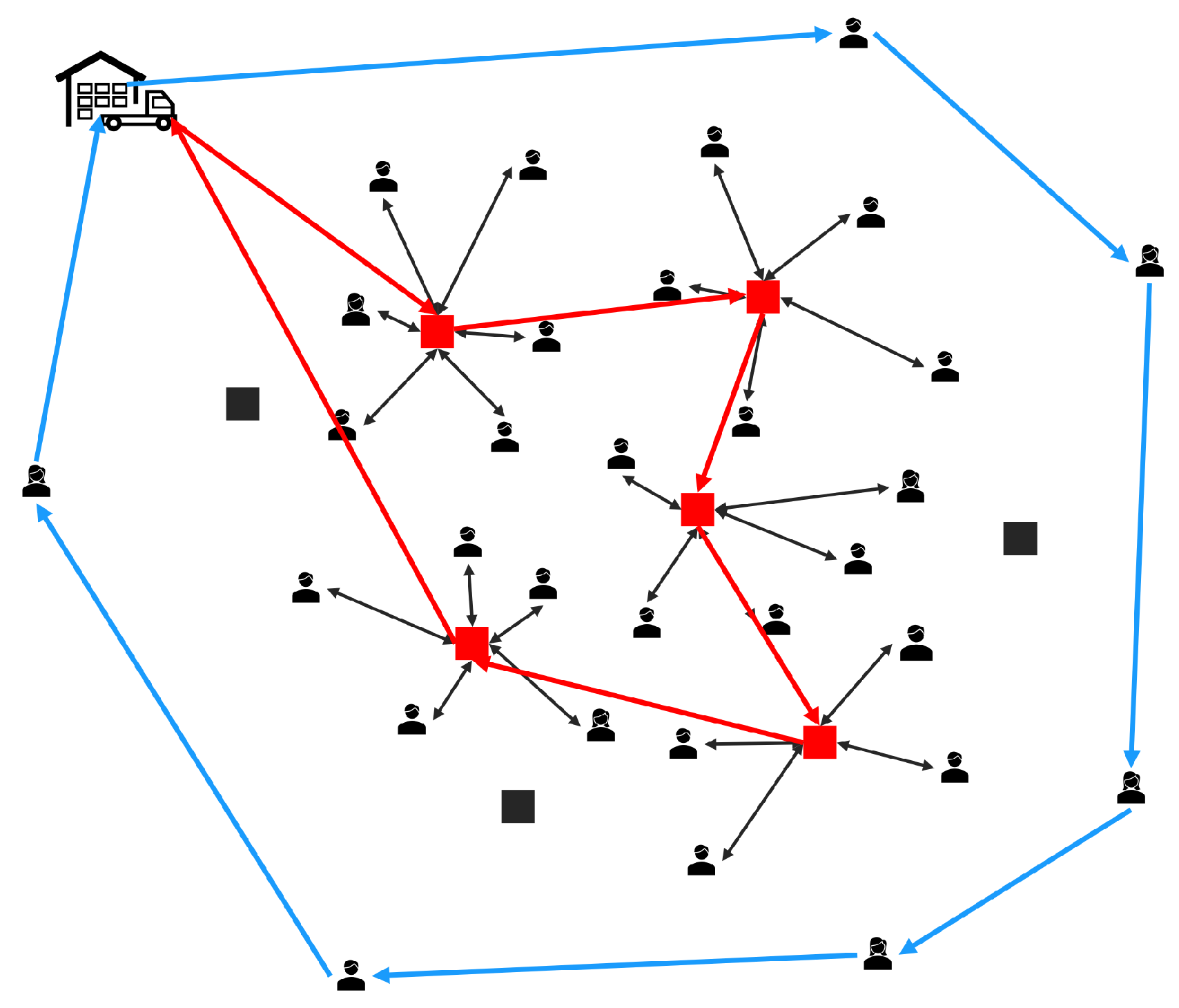
It is worth mentioning that the present research work comes from the strategic planning perspective of a company that operates in the e-commerce channel and is particularly aware of the need to ensure sustainable urban distribution. Nowadays, there are many potential customers who order various items on the Internet, and this phenomenon has been increasing in recent years [25,26]. The aim is to minimise the mobility of polluting vehicles dedicated to home delivery in urban areas, which are already affected by several polluting factors. Therefore, the focus is precisely where the company can locate and activate the $pds$ to maximise the number of customers who are able to reach the $pds$ closest to them to pick up their goods, either on foot or by nonpolluting vehicles such as bicycles or electric scooters. Of course, there may be customers located far from $pds$ or who cannot reach them sustainably and who therefore need to request a home service. In order to estimate the cost of serving all these latter customers who are not assigned to $pds$, we determine the lowest cost delivery circle, thus solving a Travelling Salesman Problem (TSP) that originates and returns to the warehouse. It will be up to the company to determine, based on the number and distance of customers to be served at home, which will be the best strategy to adopt between making a single route for delivery, or multiple routes, thus solving a VRP based on the fleet available. Figure 1 summarises a generic solution to the location-routing problem we are dealing with. It can be seen that two different circuits depart from the warehouse; one, the most external, which directly supplies customers at home; the other, more internal, which supplies the $pds$, to which customers pick up the required goods on foot or with environmentally sustainable vehicles. Isolated $pds$ (represented by squares) are those not selected.

It is worth emphasizing here the validity of the solution method, which highlights how strategic it is to determine where and how many $pds$ to locate with the objective of maximizing sustainable mobility, showing in the two circuits shown in Figure 1, how the customers to be served directly and those who will use the $pds$ are distributed. Once the company determines by which means of transport it will deliver goods to customers and $pds$, the same approach proposed here can determine the optimal VRP instead of the two circuits presently calculated. Moreover, by determining simultaneously the $pds$ to activate and the optimal tours to serve the selected $pds$ and the customers who do not go to any $pds$ it is also possible to evaluate incentive policies or discounts for customers using $pds$, as it will be explained later.

The organization of the paper is as follows. In Section 2, we introduce the proposed exact approach together with the MILP model and the required notation. Section 3 reports the results of different computational experiments. Most of them are performed based on random instances representing an urban distribution network, assuming a higher concentration of users in the centre than in the periphery. The instances generated for our tests differ in the number of customers and $pds$ and their distance from each other, and pollutant emissions, dependent on the vehicles used. In the last test, a real-size urban delivery problem in the city of Genoa is presented. Finally, in Section 4, we give some conclusions and outline future work.

2. The Proposed Exact Approach

To find the solution to the present $pds$ location-delivering problem that minimizes the total cost, given by the travelling and emission cost components, we propose an exact approach consisting of a MILP model presented in Section 2.1, and successive partitioning criteria described in Section 2.2. First, the required notation is here below reported.

• w is a node representing the warehouse from which all delivering routes depart.
• C is a finite set of customers.
• $Q\subseteq C$ is the subset of customers served by $pds$.
• $Q^{\prime }=C\backslash Q$ is the subset of customers that will not be served by $pds$.
• $\widehat{Q}$ = $C\cup \left\{w\right\}$ is a finite set of customer plus the warehouse.
• P is a finite set of pds.
• $P^{\prime }\subseteq P$ is the subset of activated $pds$.
• $\widehat{P}$ = $P\cup \left\{w\right\}$ is a finite set of $pds$ plus the warehouse.
• $r_j\ge 0$ is the capacity of $p_j$, $\forall j\in P$ defined as the maximum number of customers it can serve.
• $a_j\ge 0$ is the activation cost of $p_j$, $\forall j\in P$.
• D is the maximum distance that a user is willing to travel by nonpolluting means (e.g., on foot or bikes).
• f is the fuel cost.
• e is the air pollution emission per km.
• $d_{ij}$ is the distance to customer i from pds j.
• $d_{il}$ is the distance to customer i from customer l.
• $d_{jk}$ is the distance to pds j from pds k.
• $c_{ij}=e·2d_{ij}$ is the air pollution cost of $q_i$ from $p_j$, $\forall i\in C$, $\forall j\in P$.
• $c_{il}=d_{il}·f·e$ is the service cost of $q_i$ from $q_l$, $\forall i,l\in Q$.
• $c_{jk}=d_{jk}·f·e$ is the service cost of $p_j$ from $p_k$, $\forall j,k\in \widehat{P}$.
• $u_i$$\in {\mathbb{R}}^{+}$ is an arbitrary real numbers for the subtour elimination $\forall i\in \widehat{Q}$.
• $u_j\in {\mathbb{R}}^{+}$ is an arbitrary real numbers for the subtour elimination $\forall j\in \widehat{P}$.

All parameters are given by the benchmark problem instances. The mathematical programming formulation of the problem requires the following 4 decision variables, defined as:

$$\begin{array}{cc}\hfill x_{ij}& =\left\{\begin{array}{cc}1\hfill & \mathrm{if}\mathrm{customer}{q}_i\in C\mathrm{is}\mathrm{served}\mathrm{by}{p}_j\in P\hfill \\ 0\hfill & \mathrm{otherwise};\hfill \end{array}\right.\hfill \\ \hfill y_j& =\left\{\begin{array}{cc}1\hfill & \mathrm{if}{p}_j\in P\mathrm{is}\mathrm{activated}\hfill \\ 0\hfill & \mathrm{otherwise};\hfill \end{array}\right.\hfill \\ \hfill t_{il}& =\left\{\begin{array}{cc}1\hfill & \mathrm{if}\mathrm{the}\mathrm{path}\mathrm{from}{q}_i\in \widehat{Q}\mathrm{to}{q}_l\in \widehat{Q}\mathrm{is}\mathrm{selected}\hfill \\ 0\hfill & \mathrm{otherwise};\hfill \end{array}\right.\hfill \\ \hfill s_{jk}& =\left\{\begin{array}{cc}1\hfill & \mathrm{if}\mathrm{the}\mathrm{path}\mathrm{from}{p}_j\in \widehat{P}\mathrm{to}{p}_k\in \widehat{P}\mathrm{is}\mathrm{selected}\hfill \\ 0\hfill & \mathrm{otherwise};\hfill \end{array}\right.\hfill \end{array}$$

2.1. The Proposed Milp Model

The objective function of the model aims to minimize the overall distribution costs within an urban distribution network. In particular, it consists of the following 4 cost components (Equation (1)):

• pollutant emission from customers to $pds$,
• activation cost of the selected $pds$,
• cost of the distance traveled to serve customers not served by $pds$,
• and total distance traveled to refill the activated $pds$.

It is worth noting that in the computational tests that we will present in Section 3, component $\left(a\right)$ of the objective function (1) will have a zero contribution, setting the pollutant emission produced by customers walking or cycling to their reference $pds$ at 0. In one experiment, however, this component will be taken into account by including the same pollutant coefficient as the vehicles used by the distribution company to refuell $pds$ and non-pds users. In the latter case, the relative cost can be seen as a “saving” value on the total refuelling cost, which can then be taken into account as an incentive for customers to go directly to $pds$ instead of opting for home delivery. This possible saving and its computation will be analysed in Section 3. Then, the proposed model for solving the problem under consideration is as follows:

$$\mathit{MIN}z=\sum _{q_i\in C}\sum _{p_j\in P}{c}_{ij}{x}_{ij}+\sum _{p_j\in P}{a}_j{y}_j+\sum _{q_i\in \widehat{Q}}\sum _{q_l\in \widehat{Q}}{c}_{il}{t}_{il}+\sum _{p_j\in \widehat{P}}\sum _{p_k\in \widehat{P}}{c}_{jk}{s}_{jk}$$

(1)

Subject to the constraints:

$$\begin{array}{ccc}\hfill \sum _{p_j\in \widehat{P}}{x}_{ij}& =1\hfill & \hfill \forall q_i\in C\end{array}$$

(2)

$$\begin{array}{ccc}\hfill \sum _{q_i\in C}{x}_{ij}& \le r_j{y}_j\hfill & \hfill \forall p_j\in P\end{array}$$

(3)

$$\begin{array}{ccc}\hfill d_{ij}{x}_{ij}& \le D\hfill & \hfill \forall q_i\in C,\forall p_j\in P\end{array}$$

(4)

$$\begin{array}{cc}\hfill \sum _{i\in C}{t}_{iw}& \le 1\hfill \end{array}$$

(5)

$$\begin{array}{cc}\hfill \sum _{l\in C}{t}_{wl}& \le 1\hfill \end{array}$$

(6)

$$\begin{array}{ccc}\hfill \sum _{q_l\in \widehat{Q}|l\ne i}{t}_{il}& =x_{iw}\hfill & \hfill \forall q_i\in C\end{array}$$

(7)

$$\begin{array}{ccc}\hfill \sum _{q_i\in \widehat{Q}|l\ne i}{t}_{li}& =x_{lw}\hfill & \hfill \forall q_l\in C\end{array}$$

(8)

$$\begin{array}{ccc}\hfill u_i+\left(\right|\widehat{Q}|-1)t_{il}-\left(\right|\widehat{Q}|-2)& \le u_l\hfill & \hfill \forall i,l\in \widehat{Q}\end{array}$$

(9)

$$\begin{array}{cc}\hfill \sum _{j\in \widehat{P}}{s}_{jw}& \le 1\hfill \end{array}$$

(10)

$$\begin{array}{cc}\hfill \sum _{k\in \widehat{P}}{s}_{wk}& \le 1\hfill \end{array}$$

(11)

$$\begin{array}{ccc}\hfill \sum _{p_k\in \widehat{P}|j\ne k}{s}_{jk}& =y_j\hfill & \hfill \forall p_j\in \widehat{P}\end{array}$$

(12)

$$\begin{array}{ccc}\hfill \sum _{p_j\in \widehat{P}|j\ne k}{s}_{kj}& =y_k\hfill & \hfill \forall p_k\in \widehat{P}\end{array}$$

(13)

$$\begin{array}{ccc}\hfill u_j+\left(\right|\widehat{P}|-1)s_{jk}-\left(\right|\widehat{P}|-2)& \le u_k\hfill & \hfill \forall j,k\in \widehat{P}\end{array}$$

(14)

$$\begin{array}{ccc}\hfill x_{ij}& \in \left\{0,1\right\}\hfill & \hfill \forall i\in C,\forall j\in P\end{array}$$

(15)

$$\begin{array}{ccc}\hfill y_j& \in \left\{0,1\right\}\hfill & \hfill \forall j\in P\end{array}$$

(16)

$$\begin{array}{ccc}\hfill t_{il}& \in \left\{0,1\right\}\hfill & \hfill \forall i,l\in \widehat{Q}\end{array}$$

(17)

$$\begin{array}{ccc}\hfill s_{jk}& \in \left\{0,1\right\}\hfill & \hfill \forall j,k\in \widehat{P}\end{array}$$

(18)

Constraints (2) ensure that each customer $q_i\in C$ is either served directly by exactly one $pds$ $p_j\in \widehat{P}$, to which it goes to pick up the goods it has ordered or is served in the home delivery route that starts from the warehouse w.

Constraints (3) ensure that each $pds$ $p_j\in P$ cannot serve more customers than its capacity $r_j$. Constraints (4) impose that the distance between each customer and each $pds$ should not exceed the given maximum distance D. Constraints (5), (6), (10) and (11) ensures that from node w must leave at most one outgoing and ingoing edge, for each customer $\in C$ and $pds\in \widehat{P}$. The two different delivery tours of the goods are defined in the following constraints. Indeed, constraints (7) and (8) are the classical TSP formulation involving each customer $\in C$ served by the warehouse and defining the partitioning between the set Q and $Q^{\prime }$. Constraints (12) and (13) are the classical TSP formulation involving each $pds\in \widehat{P}$. More precisely, these constraints guarantee that each node must have only one outgoing edge and only one ingoing edge, that is each node must have a predecessor node and a successor node in the circuit. Constraints (9) and (14) are the Miller Tucker Zemlin (MTZ) formulation for the subtour elimination constraints [27]. Finally, constraints (15)–(18) define the decision variables.

2.2. The Partitioning Criteria

To obtain exact solutions of the proposed MILP model in a computationally efficient way we embed it in a branching scheme in which its solution space is partitioned according to how the sets Q and $Q^{\prime }$ are determined. More precisely, we partition the set C of customers by dividing it into two disjoint (nonoverlapping) subsets according to the following conditions:

e.

at least one customer does not go to a pickup station and is served directly by w;

f.

no customers are served by w, that is each customer has a reference pickup station close enough to pick up the ordered goods independently.

In the case $\left(e\right)$ constraints (5) and (6) of the above model are modified as follows:

$$\begin{array}{cc}\hfill \sum _{i\in C}{t}_{iw}& =1\hfill \end{array}$$

(19)

$$\begin{array}{cc}\hfill \sum _{l\in C}{t}_{wl}& =1\hfill \end{array}$$

(20)

where constraints (19) and (20) ensure that there is at least one customer served by the warehouse.

In the case $\left(f\right)$, instead, we eliminate from the objective function the costs relating to the customers served by w. Thus, we will have three cost components:

$$\mathit{MIN}z=\sum _{q_i\in C}\sum _{p_j\in P}{c}_{ij}{x}_{ij}+\sum _{p_j\in P}{a}_j{y}_j+\sum _{p_j\in \widehat{P}}\sum _{p_k\in \widehat{P}}{c}_{jk}{s}_{jk}$$

(21)

From the model described in the Section 2.1 we use the constraints: (3), (4) and (10)–(18) and we modify the constraint (2) as follows:

$$\begin{array}{ccc}\hfill \sum _{p_j\in P}{x}_{ij}& =1\hfill & \hfill \forall q_i\in C\end{array}$$

(22)

Constraint (22) is defined $\forall j\in P$; in fact, having no customers to serve from w it guarantees that all customers go to a $pds$ to pick up the ordered goods.

Then, the optimal solution of the problem is the best between the solution of the model associated with the case $\left(e\right)$, that is (1)–(4), (7)–(20) and the one associated with the case $\left(f\right)$, that is (3), (4), (10)–(16), (18), (21) and (22).

3. Computational Experimentations and Discussion of the Results

In this section, we present the results of the computational experimentation performed. Tests were carried out with the aim of supporting the decision makers of companies operating in the e-commerce to verify how the activation costs of $pds$, the distance between customers and their nearest $pds$ and the vehicle pollutant emission impact on the choice of $pds$ number and location and consequently on the total cost of the pickup and delivery process. In the computational experiments reported in the first four subsections the instances have been generated using a tournament method to obtain a greater density of customers in the center than in the peripheral zones and considering the Euclidean distance on a 3 × 3 km city area. In Section 3.5 a case study with data derived from a delivery problem involving customers in a district of the city of Genoa (Italy) is presented. All test have been run on a Windows Server 2019 Intel(R) Core(TM) i9-9820X CPU 10 cores, 20 thread, 3.30 GHz 3.31 GHz, 16 GB RAM (based in Italy). IBM ILOG CPLEX Optimization Studio 20.1.0 has been used as mixed integer linear programming solver. A time limit of 1 h have been set for solving each instance. We first performed tests by varying the number of customers from 10 to 150 and the number of $pds$ from 5 to 30. For each type of these instances we generated the activation cost of the $pds$ from 5 to 10 and their capacity from 10 to 30. More specifically, information about the customers and $pds$ of the instances considered is shown in

Table 1. Definition of the instances of the problem for the first set of computational experiments.

Type	C	P	Act	Cap
1	10	5	5–10	10–30
2	20	5	5–10	10–30
3	50	5	5–10	10–30
4	50	10	5–10	10–30
5	100	10	5–10	10–30
6	50	20	5–10	10–30
7	80	20	5–10	10–30
8	100	20	5–10	10–30
9	120	30	5–10	10–30
10	150	30	5–10	10–30

. Column headings of Table 1 are as follows. Type refers to the type of instance considered; C is the number of customers; P the number of $pds$; Act is the activation cost for each $pds$ and Cap is the capacity of each $pds$.

In the first tests we estimated the cost of air pollution to be $2.27$ €/vehicle per km, as the average air pollution for land freight transport. Of course, this value may vary depending on the type of vehicle, the load/weight of the vehicle, the fuel used and also the type of city, whether urban or suburban [28]. In this paper, we assume that deliveries are made by a light commercial vehicle (LCV), according to the standards used by the European Union to denote a commercial transport vehicle with an authorized gross weight not exceeding 3 tons. Due to the smaller size and lower carrying capacity of LCVs, their fuel consumption averages about 8–10 L/100 km. We initially assumed the cost of fuel consumption of the vehicle used by the company to be 0.1 €/L. Instead, as anticipated in the previous section, we assume equal to zero the emission cost of moving customers to/from $pds$, and thus null the component $\left(a\right)$ of the objective function $\left(1\right)$. Finally, the maximum acceptable distance for customers to go directly to pickup the ordered goods at a $pds$ is set to 850 m.

Table 2. First computational test. Results of cost component values.

Type	Total Act Cost	$\widehat{\mathit{Q}}$ Cost	$\widehat{\mathit{P}}$ Cost	Obj	CPU
1	6.28	29.01	9.22	44.52	0.16
2	12.74	32.27	14.98	60	0.19
3	19.51	80.76	19.22	119.5	33.93
4	23.71	46.02	22.38	92.12	0.9
5	40.04	53.54	33.17	126.76	15.86
6	27.31	29.79	26.48	83.59	7.61
7	36.98	31.28	33.2	101.47	60.7
8	45.22	26.57	37.34	109.13	538.22
9	51.22	15.44	43.60	110.28	1744.06
10	52.89	19.86	45.58	118.33	2004.56

reports the results obtained by solving the model reported in Section 2.2 with different instances of the problem using the above settings. In particular, Table 2 in each row shows the average results obtained by running 10 instances for each type defined above. Among the 10 instances the data that change are the activation cost of $pds$ (5–10), the $pds$ capacity (10–30), and the distance between customers and $pds$. Column headings of Table 2 are as follows. Total Act Cost is the average of the activation cost of the selected $pds$; $\widehat{\mathit{Q}}$ Cost is the average total cost to serve customers not served by $pds$; $\widehat{\mathit{P}}$ Cost is the average total cost to refill all the activated $pds$; Obj is the average value of the objective function $\left(1\right)$ of the problem and CPU is the average computational time required to find the optimal solution, expressed in seconds.

Looking at the results in Table 2, in all types of instances we obtained an optimal solution within the assumed maximum time of one hour. We can immediately see that 850 m is an ideal distance because a fair amount of $pds$ are activated. More precisely, on average 4.42 $pds$ are activated, which manage to serve approximately 85% of the customers, as can be seen from

Table 3. First computational test. Results of the selected $pds$ and served customers.

Type	Selected pds	PDS	W
1	0.9	55%	45%
2	1.8	74.5%	25.5%
3	2.6	70.6%	29.4%
4	3.2	84.4%	15.6%
5	5.3	90.7%	9.3%
6	4	90.8%	9.2%
7	5.3	93.75%	6.25%
8	6.1	95.9%	4.1%
9	7.3	98%	2%
10	7.7	98%	2%

, where the average number of selected $pds$ and the percentage of served and not served customers by the $pds$ (see columns Selected $pds$, PDS and W, respectively), are reported. Moreover, having the remaining 15% of customers to be served directly at home, we are therefore able to maintain an excellent balance of activation costs and transportation ones and above all contain the costs in terms of sustainability that we have included in the delivering cost.

After pointing out that the exact method described in Section 2 was able to find the optimal solution for all the instances considered, it is important to emphasise how the branching technique proposed in Section 2.2 resulted in a particularly significant reduction in computational time compared to using only model (1)–(18). Figure 2 shows the comparison of the computational time (second) required to find the optimal solution of the instances in Table 2 to the model alone (dashed line) and to the entire partitioning method (solid line), thus highlighting the efficiency of the proposed solution method. From Figure 2, it can also be seen that for instances of type 1 and 6, the computational time is lower than for the others, relative to the increase in their size. This is due to the very favorable ratio of these instances between the number of customers and the number of available $pds$.

3.1. Tests with and without the Cost Component of Pollutant Emissions from Customer Mobility

As a next computational test, we select the first instance of each type used in Table 2 by including the component $\left(a\right)$ in the objective function, respectively (1) and (21), of the model related to the cost of pollutant emission of the customers personally going to collect the ordered goods. In this analysis, we have assumed that customers use the same type of vehicle of the company to directly supply customers from the warehouse. This allows us to evaluate the saving between the cost of activating a $pds$ and the delivery cost more significantly.

Table 4. Results of the first instance of each type considered in Table 2 without the cost component $\left(a\right)$ of the objective function.

Instance	Total Act Cost	$\widehat{\mathit{Q}}$ Cost	$\widehat{\mathit{P}}$ Cost	Obj
1	5.49	16.18	11.16	32.83
2	5.01	26.56	10.92	42.49
3	21.31	36.97	21.29	79.56
4	18.42	36.97	21.36	76.75
5	50.14	62.00	37.07	149.22
6	25.91	21.76	26.64	74.30
7	43.07	26.76	36.89	106.72
8	47.34	15.90	37.08	100.32
9	40.85	37.45	36.64	114.94
10	56.93	0.00	41.97	98.90

shows the optimal value of the solution of the considered instances when cost component $\left(a\right)$ is not taken into account, and thus setting the emission cost to zero. The same results are shown in

Table 5. Results of the instances of Table 4 with all the cost components of the objective function.

Instance	Served C Cost	Total Act Cost	$\widehat{\mathit{Q}}$ Cost	$\widehat{\mathit{P}}$ Cost	Obj
1	2.25	5.49	16.18	11.16	35.08
2	3.52	5.01	26.56	10.92	46.02
3	9.63	21.31	36.97	21.29	89.20
4	10.95	18.42	36.97	21.36	87.70
5	18.34	50.14	62.00	37.07	167.56
6	11.24	25.91	21.76	26.64	85.54
7	15.10	38.00	37.06	31.76	121.92
8	21.16	39.86	31.77	32.00	124.79
9	21.81	44.74	32.26	41.94	140.74
10	29.39	59.32	0.00	42.05	130.75

where, to the same columns of Table 4, column Served C Cost reporting the objective function component $\left(a\right)$ is added.

It can easily be seen that up to instance 6, there is no difference between the values reported in Table 4 and Table 5. In fact, if we do not consider the Served C Cost column of Table 5, the values in the Obj columns of both tables are the same, and are related to the same activation choice of the $pds$, as it is reported in

Table 6. Results of the selected $pds$ and served customers.

Instance	Results Table 4			Results Table 5
	Selected pds	PDS	W	Selected pds	PDS	W
1	1	80%	20%	1	80%	20%
2	1	80%	20%	1	80%	20%
3	3	88%	12%	3	88%	12%
4	3	88%	12%	3	88%	12%
5	6	89%	11%	6	89%	11%
6	4	94%	6%	4	94%	6%
7	6	95%	5%	5	92.50%	7.50%
8	6	98%	2%	5	95%	5%
9	6	95%	5%	7	95.83%	4.17%
10	7	100%	0	7	100%	0

. The column headings of Table 6 are the same as those of Table 3.

Instead, in instances 7–10, we can see different values for not adding or adding, respectively, in the objective function, the cost paid by customers going to pick up their goods. More precisely, we can see that the model makes different choices in terms of activating pickup-delivery stations in the two cases based on the number of customers served. In fact, the model does not activate a $pds$ if it serves a limited number of customers compared to its capacity (Table 5), as this would be disadvantageous. Readers can observe the opposite behaviour in Table 4 and Table 6, where the model activates a pickup-delivery station even if it only serves a limited number of customers compared to its capacity. Significant, however, is the solution obtained in the case of instances 7 and 8, where the optimal solution corresponds to different choices between that made without the customer transfer costs (Table 4) and that including them (Table 5). In particular, in the first case one pickup-delivery station more than in the last case is activated. In fact, it is more cost-effective to activate an additional $pds$ (see Table 6), even if it serves only a few customers, since the total cost is more sustainable anyway. An example of this case related to instance 7 is shown in Figure 3, where a pickup-delivery station is activated despite serving only two customers.

The opposite case occurs in the same instance shown in Table 5, where having added the transport cost of customers to/from the $pds$, it is not convenient to activate an additional $pds$ when only two customers are served. In this case, in fact, it is preferable to serve customers directly from the warehouse in the route shown in Figure 4. Thus, we can say that the proposed exact approach tries to serve as many customers as possible from the $pds$, within the maximum distance and capacity constraints. In particular, it evaluates whether it is worthwhile to activate a pickup-delivery station even if the number of customers it could serve is significantly lower than its capacity, thus preferring to serve them directly within the route from the warehouse. That is why in instance 9, one more $pds$ is activated when the cost component $\left(a\right)$ is considered (see Table 6).

For a more in-depth analysis of the company’s costs, we focus on instance 8, which has a significant number of customers (100) and potential $pds$ to be activated (20). For this instance, we also considered the extreme case in which the company does not activate any $pds$ thus serving directly all customers at home in the delivery cycle departing from the warehouse. According to Formula (23), in this case the optimal solution has a total cost of z = 509.50 €, corresponding to the service cost of the customers from the warehouse given by the third component $\left(c\right)$ of the objective function (1).

$$\mathit{MIN}z=\sum _{q_i\in \widehat{Q}}\sum _{q_l\in \widehat{Q}}{c}_{il}{t}_{il}$$

(23)

Note that in (23) $\widehat{Q}$ = $C\cup \left\{w\right\}$, that is $\widehat{Q}$ includes all customers. However, note that the activation of pickup-delivery stations for customers enables the company to achieve considerable savings on the total cost. From the objective function (1) readers can note that this saving is more than 300% when considering transport costs between $pds$ and customers (i.e., 124.79 €, from Table 5) and more than 400% (i.e., 100.32 €, from Table 4) when considering them as zero, as they are carried out in a sustainable manner and with zero polluting emissions. As a final discussion about the strategic location-routing decision of the company, on the basis of the above considerations, in order to incentivise customers to use $pds$ to personally go to pick up the ordered goods by nonpolluting means, i.e., on foot, by bicycle or with electric vehicles, the company could offer customers a discount on the purchase price that could be in total at most equal to the percentage value of the savings on the company’s cost, that is up to 100% of the total cost in the case of instance 8. In fact, in this case, the company would still make a saving and above all guarantee a sustainable urban distribution plan.

After analysing the costs and evaluating the hypothesis of the convenience of activating $pds$ to favour sustainable mobility and at the same time reduce total transport costs, we conducted a computational experimentation to analyse the robustness of the optimal solutions with respect to the maximum distance of customers from the $pds$, their activation cost and the choice of vehicle used, in terms of fuel costs and polluting emissions. Based on the results shown in Table 4 and Table 5, for the next experiments we decided to use the instances of type 8 that gave us better indications for solving the problem while keeping computation times affordable. More precisely, we kept the number of customers $\left(100\right)$ and $pds$ (20) constant, while we considered variable values for the other parameters, as shown in Table 1. The fuel cost per km is 0.1 €/L and the maximum distance allowed for customers is 850 m as for the instances shown in Table 2. In particular, we performed new tests varying the following characteristics:

• the maximum allowed distance between customers and $pds$ is arbitrary assigned while $pds$ activation costs and capacity are randomly assigned in a given range. Fuel and emission cost is constant (as for Table 2);
• the emission cost is assigned depending on the type of vehicle, the fuel type and the emission class, while activation costs and capacity of the $pds$ are randomly assigned in a given range. The maximum distance is constant (as for Table 2);
• the $pds$ activation cost is arbitrary assigned, the capacity is randomly assigned in a given range and the fuel cost, emission cost and maximum distance are constant (as for Table 2).

Each value is generated randomly within the set range using the standard RNG function of the Java language $random\left(\right)$. The results and the related analysis of these experiments are reported in Section 3.2, Section 3.3, Section 3.4, respectively.

3.2. Max Distance Test

This test considers the variation of the maximum distance between customers and $pds$. We refer to 5 different cases in which we assign the following values (Max Dist in column heading of

Table 7. Maximum distance variation costs.

Max Dist	Act	$\widehat{\mathit{Q}}$ Cost	$\widehat{\mathit{P}}$ Cost	Obj	Gap	CPU
333	60.59	240.53	45.57	346.69	1%	2574.04
500	64.68	104.17	48.21	217.06	1%	2859.83
600	59.92	67.39	46.33	173.64	1%	2400.13
750	48.55	39.51	39.37	127.43	0%	312.41
1000	34.63	23.01	30.17	87.82	0%	19.57

): 333, 500, 600, 750 and 1000 m, respectively. The purpose of the test is to investigate the number of activated $pds$ as a function of the distance. Table 7 in each row shows the average values obtained by running 10 instances for each distance defined above, showing the relevant data and results that are relative to such tests. As we may notice, the distance increase corresponds to a reduction of the number of activated pickup-delivery stations, as shown in

Table 8. Selected $pds$ and percentage of served customers depending on the distance.

Selected pds	PDS	W
7.8	53.6%	46.4%
8.3	80.7%	19.3%
7.9	88%	12%
6.5	93.5%	6.5%
4.7	96.6%	3.4%

. Consequently, the overall cost for the refueling of $pds$ ($\widehat{P}$) decreases. Note also that the total cost of directly supplying customers who exceed the maximum distance decreases.

From a computational time point of view, readers can see that for the first 3 instance types we have an average optimality gap of 1%, since we were not always able to find the optimal solution within the time limit of 1 h. Note that we assume as an optimality gap the difference between the best solution found within 1 h by our proposed model and the incumbent solution, that is the current feasible best solution found during the algorithmic search procedure in the branching tree. Since 10 test instances are performed for each distance, the average optimality gap is then obtained by averaging the optimality gap of the 10 instances performed.

Finally, we can observe that as the maximum distance increases, the CPU time required to find the optimal solution significantly decreases.

3.3. Emission Cost Test

This new set of computational tests is designed to see how, if it ever is, the company’s total delivering costs change as the type of fuel used, the size of the vehicle (light or heavy vehicle), the pollutant emission class of the vehicle used, and the type of urban area considered.

Table 9. Pollutant emission cost (€-cent per vkm).

Vehicle	Fuel Type	Size	Emission Class	Metropolitan Area
LCV	Petrol		Euro 3	0.33
			Euro 4	0.22
			Euro 5	0.16
			Euro 6	0.16
	Diesel		Euro 4	3.13
			Euro 5	2.69
			Euro 6	2.19
	Electric		n.a	0.08
HGV	Diesel	Rigid ≤ 7.5 t	Euro 4	6.28
			Euro 5	7.85
			Euro 6	1.55

shows the different values considered in our instances, that summarise the cost factors for air pollution used for calculating the health and other effects. Table 9 includes the cost factors for pollutants emitted in road transport, specifically in metropolitan area, for different emission classes (see [28]).

As can be seen from

Table 10. Emission cost variation per vehicle.

Emission Cost	Act	$\widehat{\mathit{Q}}$ Cost	$\widehat{\mathit{P}}$ Cost	Obj	CPU
0.33	43.21	28.23	34.76	106.21	773.61
0.22	43.21	28.16	34.68	106.04	512.61
0.16	43.21	28.11	34.63	105.95	507.77
3.13	45.22	27.17	38.04	110.43	597.89
2.69	45.22	26.86	37.68	109.77	603.84
2.19	45.22	26.51	37.28	109.01	838.70
0.08	43.21	28.06	34.56	105.83	536.67
6.28	45.25	29.28	40.63	115.16	292.71
7.85	45.25	30.35	41.92	117.51	161.18
1.55	43.21	29.09	35.74	108.05	532.89

, the average $pds$ (column Act) activation cost changes little. In fact, from

Table 11. Results of the selected $pds$ and served customers depending on the vehicle type.

Selected pds	PDS	W
5.9	95.3%	4.7%
5.9	95.3%	4.7%
5.9	95.3%	4.7%
6.1	95.9%	4.1%
6.1	95.9%	4.1%
6.1	95.9%	4.1%
5.9	95.3%	4.7%
6.1	95.9%	4.1%
6.1	95.9%	4.1%
5.9	95.3%	4.7%

we note that the average number of selected pickup-delivery stations is 6 and the number of customers reaching the $pds$ is 95.6%, while those served directly are only 4.4%. Obviously, the costs of the $\widehat{Q}$ and $\widehat{P}$ paths change, as they depend on the type of emission cost that is considered in the instances. In particular, the best solution, both in terms of environmental quality and costs, corresponds to the scenario in which the company uses electric vehicles to serve those customers who are unable to reach the pickup-delivery stations. Instead, the worst situation occurs when a HGV (Heavy Goods Vehicle) of Euro 5 diesel emission class is used. From a computational time point of view, note that in all instances we were able to get the optimal solution in less than 13 min. In fact, it can be seen from Table 10 that the test requiring the most computational time is the one shown in the sixth row, for which 838.70 s, equivalent to 13 min, were needed to obtain the optimal solution.

3.4. Pds Activation Test

As for the last test, concerning the sensitivity of the solutions with respect to the variation of the activation cost of $pds$, we consider 9 different cases in which we assign the following values to the activation cost of each pick-up station: 2.25, 5, 7.5, 10, 20, 30, 40, 50 and 100 €, respectively.

Table 12. Cost components of the objective function as the cost of activating $pds$ changes.

ActCost	Act	$\widehat{\mathit{Q}}$ Cost	$\widehat{\mathit{P}}$ Cost	Obj	CPU
2.25	16.65	14.04	44.00	74.69	2134.40
5	33.00	20.82	39.89	93.71	1332.28
7.5	45.75	26.04	37.33	109.12	709.74
10	54.00	36.61	33.71	124.32	772.11
20	84.00	57.21	27.50	168.70	464.81
30	102.00	81.41	23.30	206.71	469.07
40	124.00	93.00	21.74	238.73	450.31
50	145.00	102.05	20.70	267.75	456.26
100	200.00	165.56	16.04	381.60	1287.31

shows the data and results for these tests. Note that in all instances we were able to get the optimal solution in less than 35 min.

It can be seen that an increase in the cost of $pds$ corresponds, as expected, to a lower number of activated $pds$ (

Table 13. Selection of $pds$ activated and number of customers served as $pds$ activation cost changes.

Selected pds	PDS	W
7.4	98.1%	1.9%
6.6	97%	3%
6.1	96%	4%
5.4	93.9%	6.1%
4.2	90%	10%
3.4	85.2%	14.8%
3.1	82.9%	17.1%
2.9	81.1%	18.9%
2	68.5%	31.5%

). In fact, with higher activation costs, it is cheaper to serve customers directly from the warehouse. Particular attention should be paid to the values obtained with the last type of instances, where the cost of activating $pds$ is set at 100. In this case, in fact, only two $pds$ are activated, being very expensive, even if they allow only less than 70% of the customers to be served, due to the constraint on their maximum capacity. Consequently, more than 30% of customers are served directly from the warehouse. As a result, the routing cost for serving the customers ($\widehat{Q}$ Cost) increases, while the routing cost to supply $pds$ decreases.

3.5. A Real-Size Case Study

We now present a case study that was approached using the exact method proposed in Section 2, after the computational tests performed in the previous subsections. To test a realistic instance, we considered a company operating in the business of distributing products ordered through electronic channels. Due to the increasing volume of parcels to be handled, the company decided to evaluate the use of pickup-delivery stations to improve service and reduce total delivery costs. The customers associated with the service are 49 offices, located in the city district of Genoa, Italy, shown in Figure 5. We extracted customer location data from OpenStreetMap [29] along with data on the delivery points currently active in this district, i.e., post offices, to identify 19 potential pickup-delivery stations. In Figure 5, the customers are represented by blue dots, the warehouse by a yellow diamond, and the black diamonds represent the possible delivery points.

We derived the cost of service of these active delivery points based on their annual rental cost and set the activation cost of each $pds$ at €1.000. Transportation costs are the same as those used in previous tests. The distances between nodes were calculated on the urban transportation network for road vehicles and were extracted from OpenStreetMap through QGIS software [30], which allows access and download of various types of geospatial data. As before, we set the maximum allowed distance between clients and $pds$ to 850 m.

First, we calculated the total delivery cost of the company in the scenario in which it does not activate any $pds$, thus directly serving all customers from the warehouse. In this case, we used the objective function (23) and the resulting cost was €128,670.42.

Table 14. Cost components of the objective function.

Act	$\widehat{\mathit{Q}}$ Cost	$\widehat{\mathit{P}}$ Cost	Obj
8.000	67,839.59	34,604.48	110,444.08

, on the other hand, reports the optimal solution obtained using the proposed exact method, in which 8 pickup-delivery stations are activated, in yellow depicted in Figure 6. These activated $pds$ serve 48.97% of the customers, while the remaining 51.02% are served by the warehouse.

As an additional information, the computational time to find the optimal solution was about 28 min. Although the costs used in this test were not the company’s actual costs, but only an estimate based on online information, the analysis allowed us to suggest activating some $pds$ at strategic points in the considered district of the city. As a result, customers experience shorter wait times, faster delivery, greater sustainability, and lower costs.

4. Conclusions

In this paper, we addressed a variant of the multifacility location-routing problem from the perspective of a business-to-consumer company operating in an urban area. The goal was to minimize the cost of the overall pickup and delivery process with the need to determine environmentally sustainable distribution plans, thus minimizing pollutant emissions. Therefore, we must find the right balance between the number of pickup-delivery stations for goods collected directly from customers and the number of customers served at home. From a strategic point of view, we wanted to verify how the location choices of the pickup-delivery stations vary according to the maximum distance a customer is willing to walk and/or the length and cost of the route to deliver the ordered goods. The activation cost of the pickup-delivery stations also influenced the optimal solution as well as the type of vehicle used by the company. To solve this problem, we presented a novel exact approach based on the partitioning of the research space of the solutions of a MILP model. In particular, a branching constraint allowed us to split the set of customers into two subsets and consequently define the route that served the selected pickup-delivery stations and the route, if any, that served customers who do not go to any pickup-delivery station. The computational tests performed, based on randomly generated instances of up to 150 customers and 30 pickup-delivery stations, demonstrated the effectiveness of the proposed exact method in terms of both quality of the solution and calculation time. In fact, Table 2, Table 4, Table 10 and Table 12 show that in all tests performed, the optimal solution was obtained within 35 min. Only in the test to check the impact of the variation of the maximum distance accepted by customers to personally collect the ordered goods, in 3 types of instances a solution was obtained with a deviation of 1% from the optimal value of the objective function of the model within the maximum calculation limit of 1 h. In the same tests, we were able to establish that there is a threshold value for both the aforementioned distance and the cost associated with pickup-delivery stations, beyond which home delivery is more cost-effective for the company than setting up additional pickup-delivery stations. Moreover, the application of the proposed exact method to a case study related to a distribution problem in a district of the city of Genoa confirms its validity to be used for addressing real-size urban delivery problems with the goal of minimizing pollutant emissions. Finally, we were able to evaluate incentives for customers to use the pickup-delivery stations to serve themselves while ensuring savings for the company, especially in terms of environmental sustainability.

It is our intention to develop the research in two directions. First, the present problem will be applied to urban and metropolitan realities with high population density. This step will require the extrapolation of georeferenced data using appropriate software environments, such as QGIS, and interfacing the information with the model proposed here. Second, we will develop mat-heuristics to be integrated with the exact branching approach. In this case, it will be necessary to perform numerous computational tests and be able to find similar heuristics proposed in the literature applied to similar problems to validate and compare the performance of the proposed solution methods.

References

- Cano, J.A.; Londoño-Pineda, A.; Rodas, C. Sustainable Logistics for E-Commerce: A Literature Review and Bibliometric Analysis. Sustainability 2022, 14, 12247. [Google Scholar] [CrossRef]
- Dekker, R.; Bloemhof, J.; Mallidis, I. Operations Research for green logistics—An overview of aspects, issues, contributions and challenges. Eur. J. Oper. Res. 2012, 219, 671–679. [Google Scholar] [CrossRef] [Green Version]
- Bektaş, T.; Ehmke, J.F.; Psaraftis, H.N.; Puchinger, J. The role of operational research in green freight transportation. Eur. J. Oper. Res. 2019, 274, 807–823. [Google Scholar] [CrossRef] [Green Version]
- Heshmati, S.; Verstichel, J.; Esprit, E.; Vanden Berghe, G. Alternative e-commerce delivery policies: A case study concerning the effects on carbon emissions. Eur. J. Transp. Logist. 2019, 8, 217–248. [Google Scholar] [CrossRef]
- Nathanail, E.; Gogas, M.; Adamos, G. Smart Interconnections of Interurban and Urban Freight Transport towards Achieving Sustainable City Logistics. Transp. Res. Procedia 2016, 14, 983–992. [Google Scholar] [CrossRef] [Green Version]
- Behnke, M.; Kirschstein, T. The impact of path selection on GHG emissions in city logistics. Transp. Res. Part E Logist. Transp. Rev. 2017, 106, 320–336. [Google Scholar] [CrossRef]
- Carrabs, F.; Cerulli, R.; Sciomachen, A. An exact approach for the grocery delivery problem in urban areas. Soft Comput. 2017, 21, 2439–2450. [Google Scholar] [CrossRef]
- Makarova, I.; Shubenkova, K.; Mavrin, V.; Boyko, A.; Katunin, A. Development of sustainable transport in smart cities. In Proceedings of the 2017 IEEE 3rd International Forum on Research and Technologies for Society and Industry (RTSI), Modena, Italy, 11–13 September 2017; pp. 1–6. [Google Scholar]
- Cerulli, R.; Dameri, R.P.; Sciomachen, A. Operations management in distribution networks within a smart city framework. IMA J. Manag. Math. 2018, 29, 189–205. [Google Scholar] [CrossRef]
- Strale, M. Sustainable urban logistics: What are we talking about? Transp. Res. Part A Policy Pract. 2019, 130, 745–751. [Google Scholar] [CrossRef]
- Cerrone, C.; Sciomachen, A. Urban goods distribution plans to minimize transportation costs and pollutant emissions. Soft Comput. 2022, 26, 10223–10237. [Google Scholar] [CrossRef]
- Matemilola, S.; Fadeyi, O.; Sijuade, T. Paris Agreement. Encyclopedia of Sustainable Management; Springer: Cham, Switzerland, 2020; pp. 1–5. [Google Scholar]
- Wang, M.; Zhang, C.; Bell, M.G.; Miao, L. A branch-and-price algorithm for location-routing problems with pick-up stations in the last-mile distribution system. Eur. J. Oper. Res. 2022, 303, 1258–1276. [Google Scholar] [CrossRef]
- He, Y.; Wang, X.; Lin, Y.; Zhou, F.; Zhou, L. Sustainable decision making for joint distribution center location choice. Transp. Res. Part D Transp. Environ. 2017, 55, 202–216. [Google Scholar] [CrossRef]
- Deutsch, Y.; Golany, B. A parcel locker network as a solution to the logistics last mile problem. Int. J. Prod. Res. 2018, 56, 251–261. [Google Scholar] [CrossRef]
- Savelsbergh, M.W.; Sol, M. The general pickup and delivery problem. Transp. Sci. 1995, 29, 17–29. [Google Scholar] [CrossRef] [Green Version]
- Karaoglan, I.; Altiparmak, F.; Kara, I.; Dengiz, B. A branch and cut algorithm for the location-routing problem with simultaneous pickup and delivery. Eur. J. Oper. Res. 2011, 211, 318–332. [Google Scholar] [CrossRef]
- Zhou, L.; Wang, X.; Ni, L.; Lin, Y. Location-routing problem with simultaneous home delivery and customer’s pickup for city distribution of online shopping purchases. Sustainability 2016, 8, 828. [Google Scholar] [CrossRef] [Green Version]
- Yu, V.F.; Susanto, H.; Yeh, Y.H.; Lin, S.W.; Huang, Y.T. The Vehicle Routing Problem with Simultaneous Pickup and Delivery and Parcel Lockers. Mathematics 2022, 10, 920. [Google Scholar] [CrossRef]
- Bonomi, V.; Mansini, R.; Zanotti, R. Last Mile Delivery with Parcel Lockers: Evaluating the environmental impact of eco-conscious consumer behavior. IFAC-Papers OnLine 2022, 55, 72–77. [Google Scholar] [CrossRef]
- Wu, J.; Liu, X.; Li, Y.; Yang, L.; Yuan, W.; Ba, Y. A Two-Stage Model with an Improved Clustering Algorithm for a Distribution Center Location Problem under Uncertainty. Mathematics 2022, 10, 2519. [Google Scholar] [CrossRef]
- Yıldız, B.; Arslan, O.; Karaşan, O.E. A branch and price approach for routing and refueling station location model. Eur. J. Oper. Res. 2016, 248, 815–826. [Google Scholar] [CrossRef] [Green Version]
- Bao, Z.; Xie, C. Optimal station locations for en-route charging of electric vehicles in congested intercity networks: A new problem formulation and exact and approximate partitioning algorithms. Transp. Res. Part C Emerg. Technol. 2021, 133, 103447. [Google Scholar] [CrossRef]
- Farzadnia, F.; Lysgaard, J. Solving the service-oriented single-route school bus routing problem: Exact and heuristic solutions. Eur. J. Transp. Logist. 2021, 10, 100054. [Google Scholar] [CrossRef]
- Pahwa, A.; Jaller, M. A cost-based comparative analysis of different last-mile strategies for e-commerce delivery. Transp. Res. Part E Logist. Transp. Rev. 2022, 164, 102783. [Google Scholar] [CrossRef]
- Al Mashalah, H.; Hassini, E.; Gunasekaran, A.; Bhatt, D. The impact of digital transformation on supply chains through e-commerce: Literature review and a conceptual framework. Transp. Res. Part E Logist. Transp. Rev. 2022, 165, 102837. [Google Scholar] [CrossRef]
- Miller, C.E.; Tucker, A.W.; Zemlin, R.A. Integer programming formulation of traveling salesman problems. J. ACM 1960, 7, 326–329. [Google Scholar] [CrossRef]
- Van Essen, H.; Van Wijngaarden, L.; Schroten, A.; Sutter, D.; Bieler, C.; Maffii, S.; Brambilla, M.; Fiorello, D.; Fermi, F.; Parolin, R.; et al. European Commission, Directorate-General for Mobility and Transport. In Handbook on the External Costs of Transport: Version 2019—1.1; Publications Office of the European Union: Brussels, Belgium, 2020. [Google Scholar] [CrossRef]
- OpenStreetMap Contributors. 2015. Available online: https://planet.openstreetmap.org (accessed on 20 March 2023).
- QGIS. Available online: https://www.qgis.org/it/site/ (accessed on 20 March 2023).
Figure 1.
An example of solution of the present location-routing problem.
Figure 2.
Comparison of the CPU time required by the model and the whole exact approach.
Figure 3.
Example derived from Instance 7 from Table 4 without service cost of the customers.
Figure 4.
Example derived from Instance 7 from Table 5 with service cost of the customers.
Figure 5.
Urban area of the case study with the location of customers and .
Figure 6.
Activated pickup-delivery stations in the optimal solution.