
Non-Convex Particle-in-Cell Model for the Mathematical Study of the Microscopic Blood Flow

1
Applied Mathematics Laboratory, School of Science and Technology, Hellenic Open University, 26222 Patras, Greece
2
School of Applied Mathematical and Physical Sciences, National Technical University of Athens, 15780 Athens, Greece
*
Author to whom correspondence should be addressed.
Mathematics 2023, 11(9), 2156; https://0-doi-org.brum.beds.ac.uk/10.3390/math11092156
Submission received: 16 March 2023
/
Revised: 26 April 2023
/
Accepted: 28 April 2023
/
Published: 4 May 2023
(This article belongs to the Special Issue Applications of Partial Differential Equations in Mathematical Physics, 1st Edition)
Abstract
:The field of fluid mechanics was further explored through the use of a particle-in-cell model for the mathematical study of the Stokes axisymmetric flow through a swarm of erythrocytes in a small vessel. The erythrocytes were modeled as inverted prolate spheroids encompassed by a fluid fictitious envelope. The fourth order partial differential equation governing the flow was completed with Happel-type boundary conditions which dictate no fluid slip on the inverted spheroid and a shear stress free non-permeable fictitious boundary. Through innovative means, such as the Kelvin inversion method and the R-semiseparation technique, a stream function was obtained as series expansion of Gegenbauer functions of the first and the second kinds of even order. Based on this, analytical expressions of meaningful hydrodynamic quantities, such as the velocity and the pressure field, were calculated and depicted in informative graphs. Using the first term of the stream function, the drag force exerted on the erythrocyte and the drag coefficient were calculated relative to the solid volume fraction of the cell. The results of the present research can be used for the further investigation of particle–fluid interactions.
Keywords:
Stokes flow; red blood cell; particle-in-cell model; Kelvin inversion; Happel-type boundary conditionsMSC:
35Q30; 35Q35; 35G15; 35J40; 76D071. Introduction
Blood cell malfunction can cause diseases such as cardiovascular disease, hematological disease, and cancer, due to the damage caused by the mechanical stresses exerted on them [1]. The mechanical properties of a single cell can be used as biomarkers. Various experimental methods, e.g., atomic force microscopy, are used to measure the induced stress or strain on an individual cell, but the scale up to many cells cannot be obtained experimentally by conventional methods and, thus, high throughput methods are needed [2]. Towards this direction, mathematical models have proven to be a powerful theoretical tool, since the scale up or the scale down can be achieved via analytical methods.
Among them, particle-in-cell models have been used since the middle of the twentieth century, mostly in engineering problems dealing with particle–fluid interactions in swarms of particles, such as sedimentation, fluidization, and the flow of biological fluids. Through these models, analytical expressions of the macroscopic behavior of the fluid flow can be extracted from the study of the microscopic flow problem scaled down to a unitary cell that consists of a single particle surrounded by a fluid envelope. The disturbance that the other particles of the swarm cause to the flow is modeled by considering a fictitious fluid boundary of the envelope. The solid/fluid fraction of the swarm defines the thickness of this fluid envelope. The analytical determination of the flow field allows the straightforward calculation of quantities of physical, medical, and engineering interest, such as the vorticity field, the drag force acting on each particle and the macroscopic pressure gradient. These can also be used in the study of heat and mass transport processes and phenomena, such as reaction, diffusion, and adsorption.
Among the different geometrical descriptions that have been adopted for the particle-in-cell model, the spherical configuration is the most used, since it allows simpler mathematical expressions [3]. A spherical in-cell model was developed in [4] to model Stokes flow in a spherical cavity by introducing a porous spherical particle, while Faltas and Saad [5] used a particle-in-cell spherical model to describe creeping flow past slip eccentric spherical in-cell models. In [4,5] both Happel and Kuwabara conditions were applied. Sherif et al. [6] used a spherical in-cell model in order to study the interaction between two rigid spheres with slip surfaces when moving in a micropolar fluid.
With regard to the flow characteristics, the viscous forces dominate the inertial ones and thus the flow is creeping, which is indicated by a Reynolds number smaller than unity. Assuming also a steady state, the governing Navier–Stokes equation reduces to the known system of partial differential equations,
namely, Stokes equations [7,8], where denotes the position vector, is the dynamic viscosity, is the biharmonic velocity field and P stands for the harmonic pressure field.
Moreover, Papkovich–Neuber [9] proved that two harmonic potentials, fully describe the flow via the system,
When the direction of the flow is parallel to the axis of the spheroidal cell, the flow is considered to be axisymmetric, and thus a very good approximation of the real problem is provided [9], allowing the reduction of the three-dimensional problem to a two-dimensional one, practically. By introducing a scalar function, namely a stream function, the Stokes flow equations are induced to a fourth order of elliptic-type partial differential equation for the stream function [3,10] that governs the incompressible creeping axisymmetric flow.
The problem at hand is completed by setting appropriate boundary conditions. These can be of either Happel [11] or Kuwabara [12] type. According to the Happel model [11], the fluid is at rest and the spherical particle moves at a constant velocity within the fluid envelope, while in the Kuwabara model [12], the particle is stationary and the fluid flow within the cell is moving with the same constant velocity as the one imposed for the main stream. Moreover, in the Happel-type model, no shear stress condition is imposed in the external boundary, while in the Kuwabara model, nil vorticity is assumed. These differences indicate two different conditions, respectively: (a) the model is self sufficient with regard to mechanical energy and (b) the model allows the exchange of mechanical energy between the cell and the environment.
In many cell-in-cell fluid models, numerical methods are employed in order to reach to a solution. These also provide a basis for numerical implementations [13,14] and a mean for the assessment of existing numerical results. Despite the advantages of the numerical methods (e.g., geometrical flexibility, solvability in many kind differential equations, and boundary value problems), the analytical solutions provide qualitative results revealing or highlighting the geometrical and the physical characteristics of the flow. Indicatively, Datta and Deo [15] used the Kuwabara BCs for numerically solving the creeping flow around a sphere, while Madasu [16] studied numerically the flow of a sphere with slip boundary conditions considered in a spherical in-cell model. Furthermore, when a deformation of the RBCs is also taken into account, the corresponding flow problem is mostly numerically simulated [17,18,19,20]. Numerical procedures are beyond the scope of the present study.
Dassios et al. [21] advanced the spherical particle-in-cell models by augmenting the geometrical complexity from a spherical (symmetrical case) to a spheroidal one—prolate and oblate (axis-symmetry). This consequently increased the difficulty of the derivation of the analytical solution governing the flow, which was tackled by introducing the notion of the semiseparation of variables [22], according to which the stream function was given through the series expansion of specific combinations of Gegenbauer functions [23] of mixed order. Sherif et al. [24], with a spheroidal particle-in-cell model, solved the Stokes flow of a micro-polar fluid past an assemblage of spheroidal particle-in-cell models with slip boundary conditions. Recently [25], a particle-in-cell model in prolate geometry was developed using the Papkovich–Neuber representation and the non-axisymmetric flow fields were obtained in terms of harmonic functions.
With regard to blood flow, we recall that, at a microscopic level, the blood is considered to be a suspension of three types of cells—namely the erythrocytes or red blood cells (RBCs), the white blood cells, and the platelets—within an incompressible fluid, the blood plasma, the rheological behavior of which in small vessels is characterized as Newtonian. Since both the blood plasma and the RBCs constitute about of the volume of the blood [26], and due to the role RBCs play in the health condition of human organisms, the study of their flow is expected to provide important information for medical use.
The RBC is geometrically modeled as a biconcave disk [17,18,20], with a major diameter of about 8 μm and a thickness of at least 2 μm [27]. Therefore, it is mathematically represented by an inverted prolate spheroid. It was further assumed that it moves with a constant velocity U along its axis of symmetry within a Newtonian fluid, being at rest. No shape deformations of the RBC were considered. The process was modeled as a Stokes flow problem [28] for the translation of a rigid inverted prolate spheroid within a quiescent unbounded viscous fluid, which was justified by considering the rheological properties of the blood plasma and the geometrical characteristics of the RBC [26].
Dassios et al. [29] and Hadjinicolaou et al. [30] employed the Kelvin transformation for obtaining the solution of the relative movement of the erythrocytes or red blood cells within the blood plasma, representing the biconcave shape of the RBC with an inverted prolate spheroidal surface. Furthermore, Hadjinicolaou and Protopapas [31] proposed a Stokes flow model for the study of the blood plasma flow through a swarm of RBCs, in line with the particle-in-cell concept. It consists of an inverted prolate spheroid resembling the RBC and a confocal fluid envelope representing the plasma. The boundary conditions were those of Kuwabara’s type particle-in-cell model [12], expressing non slip flow on the impenetrable interior inverted prolate spheroid, while a uniform flow velocity and nil fluid vorticity were assumed on the fictitious exterior boundary. Their solution employed the R-semiseparation method, which they introduced in [32]. For an extensive literature review, one may see [21] and the references therein.
In the present manuscript, we introduce the Happel type particle-in-cell model and employing the Kelvin inversion and the semiseparation of variables technique, we solve a Stokes flow problem for a swarm of erythrocytes moving through the blood plasma.
The structure of the manuscript is as follows. In Section 2, the physical problem is mathematically formulated and the solution is derived. In Section 3, the results are discussed and sample calculations for the stream function and analytical expressions for the velocity field, the frag force and the drag coefficient are obtained, while Section 4 contains the conclusions of the present research.
2. Mathematical Formulation and Solution
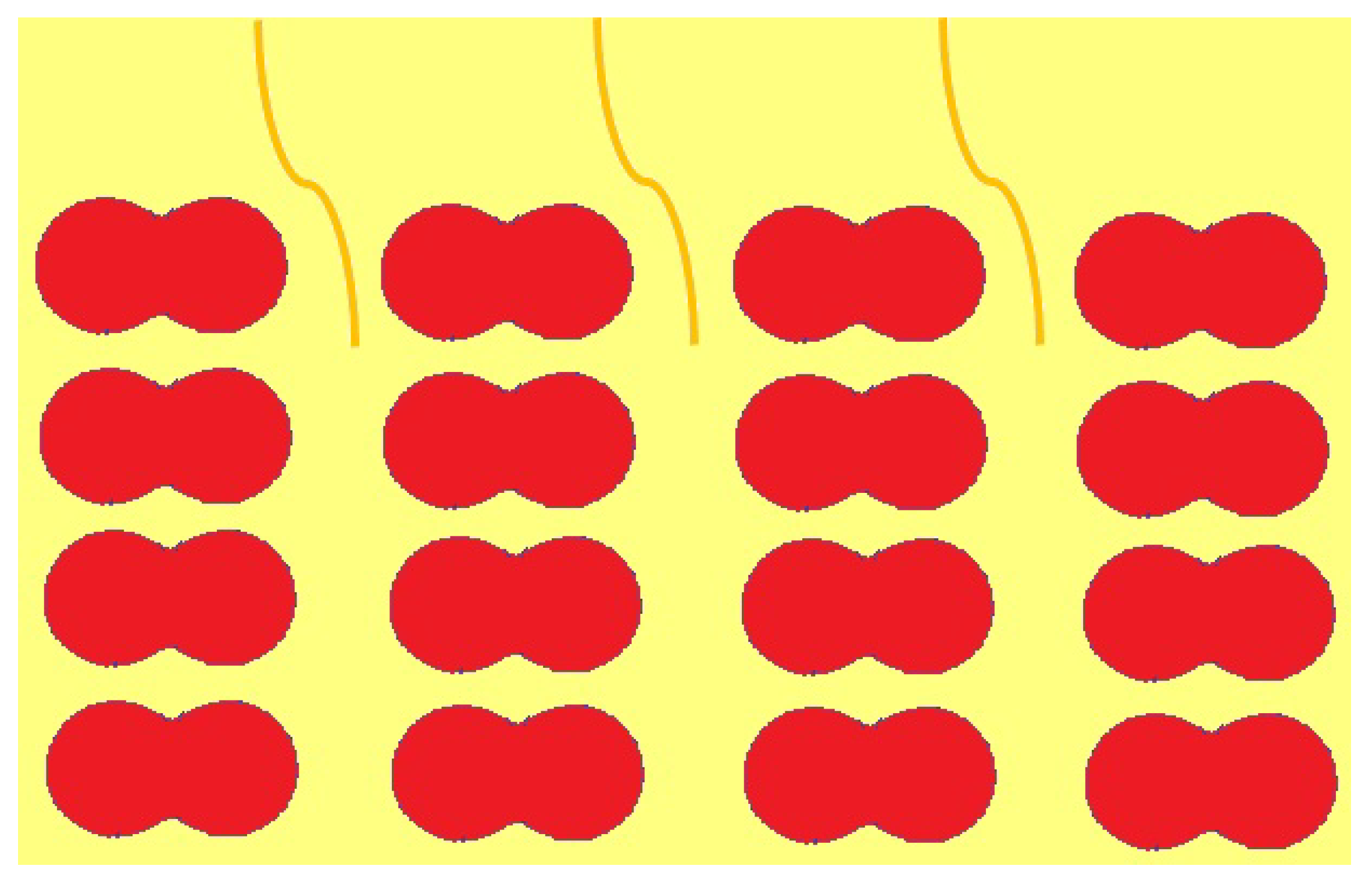
A particle-in-cell model is used in order to describe the relative flow of the blood plasma through a swarm of red blood cells (Figure 1). For the problem at hand, we consider two confocal inverted prolate spheroidal surfaces (Figure 2). The inner one, representing the RBC, is assumed to be solid moving with a velocity in the positive direction of The exterior one, stands for the fictitious fluid boundary of the particle-in-cell model.
Assuming that the flow is creeping, i.e., the inertial forces dominate over the viscous ones, which is denoted by a Reynolds number much less than unity and taking into account the imposed axial symmetry of the physical and the geometrical model with respect to axis, the governing equation for the Stokes flow problem is described by the fourth order partial differential equation,
where is the Stokes operator, is the position vector, is the flow field, and is the corresponding stream function.
Boundary conditions of Happel’s type model [11] imposes non-slip conditions on the solid surface which are expressed by the following equations:
where are the dimensionless velocity’s components and are the unit vectors in the inverted prolate spheroid coordinate system and [33].
Moreover, on the fluid surface, Happel’s model assumes that there is no flow across the boundary, i.e.,
and zero tangential shear stress, i.e.,
where is the dimensionless tangential stress [3].
Furthermore, denoting by the solid volume fraction of the cell, the volume of the cell and the volume of the solid, the connecting relation is
through which the exterior inverted prolate spheroid is defined.
In the inverted prolate spheroidal coordinates where and denotes the semifocal distance, the Stokes operator is given as:
The BCs (4) through (7) are expressed in the inverted prolate spheroidal geometry via the following relations: (10)–(13).
where represent the surfaces respectively.
Summarizing, the problem at hand is defined via Stokes Equation (3), with boundary conditions (10)–(12), and (14).
A straightforward attempt to solve the problem via the separation of variables method encountered significant difficulties that did not allow the derivation of the eigenfunctions of kernel space of In order to overcome these difficulties, the Kelvin inversion method was employed aiming to transform the problem to an equivalent one for which separable solutions could be obtained. According to this, every vector defined in a domain V is transformed to a new one , defined in a domain which is the Kelvin image of the initial V, such as
where is the radius of the inversion sphere and (Figure 3).
In the present work, Kelvin’s inversion method was used and the initial domain between the two confocal inverted prolate spheroids, was transformed in a new domain V, which is the domain between two confocal prolate spheroids. This way, we transformed the inverted prolate spheroidal cell model (non-convex cell) to a prolate spheroidal one (convex cell), which allowed the use of the analytical results obtained for an analogous problem in the prolate spheroidal geometry (Figure 4).
In regard to the stream function, Dassios in [34] proved that the steam function is related to the stream function , describing the flow between the two prolate spheroids via the equation
or equivalently,
where denote the prolate spheroidal coordinates, where and are connected [29] with the inverted spheroidal ones via the relations
where
Consequently, Kelvin’s inversion method transforms the problem at hand into the following:
where express the surfaces of the external and the internal spheroid, respectively.
The solution of (20) is derived using the concept of semiseparation [22], according to which the stream function assumes the form
where are Gegenbauer functions of the first and the second kind, respectively [23], and are particular linear combinations of Gegenbauer functions.
Matching the specific characteristics of the flow expressed through the BCs, and those of the Gegenbauer functions, the stream function assumes the form
where
and for ,
The coefficients should be calculated by applying the BCs. Since the resulting linear system is infinite, a cut-off technique is applied. We observe that for the linear system has equations and unknowns. Therefore an extra condition is needed in order to reach at a solvable square system. This condition is obtained by requiring that the solution for the spheroidal-in-cell model tends to the one in the sphere-in-cell model, when the semifocal distance tends to zero, which sets equal to zero the constant This condition creates a linear system for the unknown coefficients.
Employing the obtained expression for the stream function hydrodynamic quantities such us the velocity components and the pressure gradient P are derived [3] through the relations
where is the shear viscosity of the fluid.
The drag force [3] exerted from the inverted prolate spheroid to the fluid is
where are two points on the meridian plane and the integration is from point A through point B and, if R is the reference area, is the mass density of the fluid, the drag coefficient is
Since the Reynolds number is defined as
the drag coefficient (34) assumes the form
where L is the characteristic length.
3. Results and Discussion
Approximating the stream function using only the first term of the series expansion, the stream function assumes the form
which is a plausible assumption, as most of the fundamental characteristics of the flow seem to be contained in the leading term.
Moreover, the unknown coefficients in (40) by applying the BCs (4)–(7) can be calculated through the system
where
and the Gegenbauer functions of the first kind appeared above are
while the one of the second kind is
Consequently, the first order approximation, of the solution series is
In order to depict streamlines, we used the relations that connect each one of the prolate spheroidal coordinates with the inverted prolate spheroid coordinates which are derived from (18), (19) via the relations
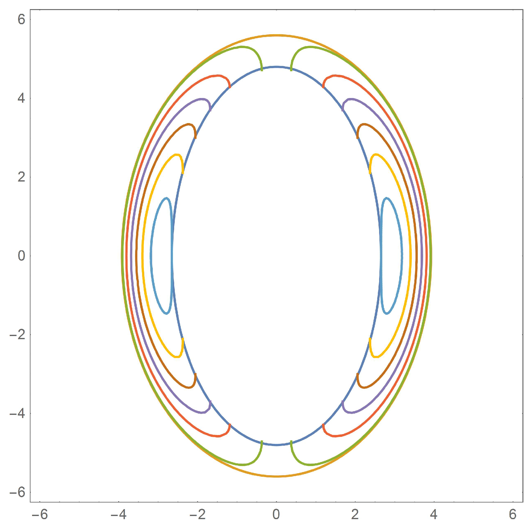
In Figure 5, Figure 6 and Figure 7 we depict streamlines in the plane for the stream function with values and and (from the outer to the inner prolate spheroid), respectively, setting in all cases
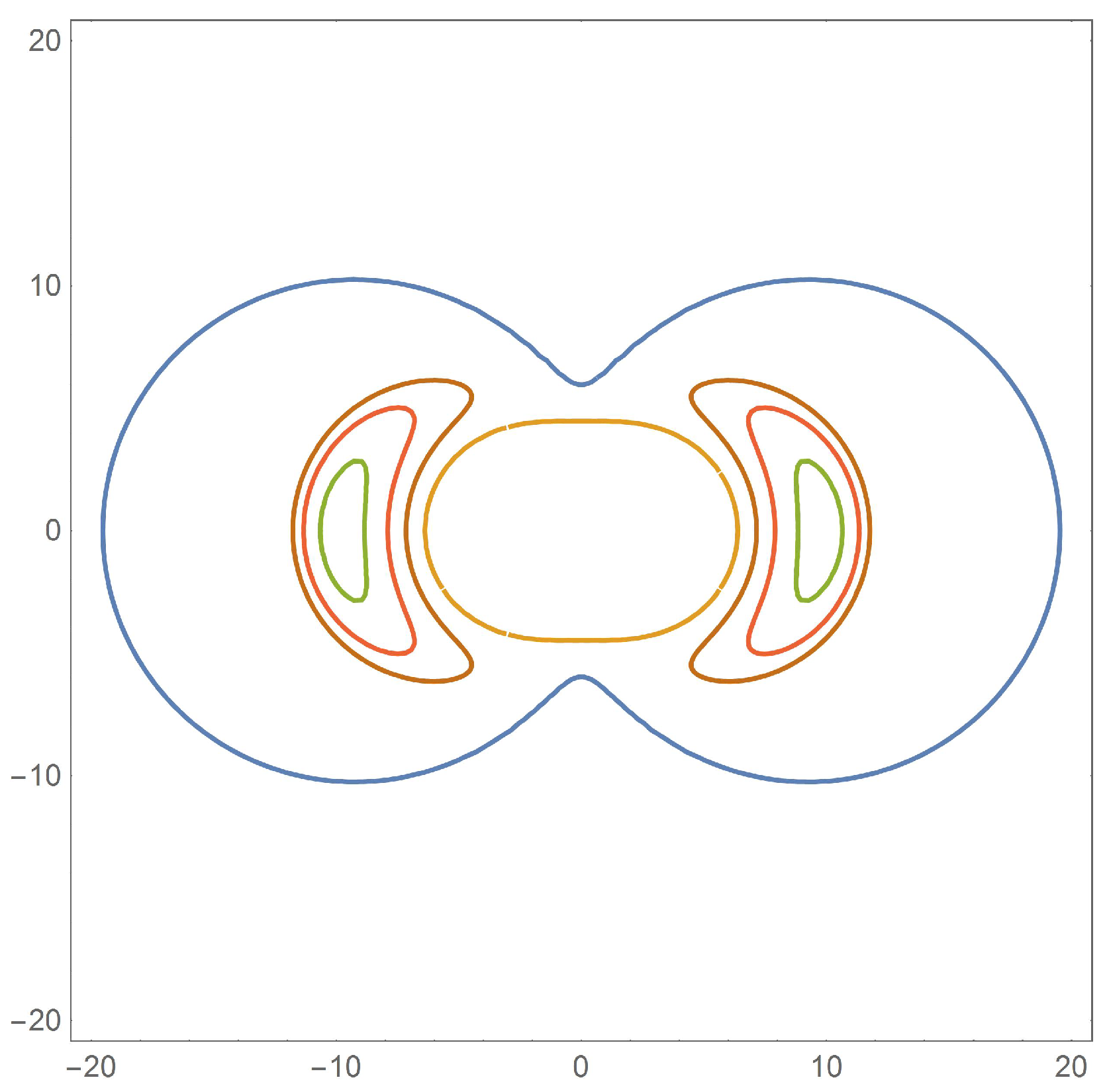
In Figure 8, Figure 9 and Figure 10, we depict streamlines for the stream function , assuming the values and 50, and (from the outer to the inner inverted prolate spheroid) respectively, using in all cases while the solid volume fraction of the cell, is and respectively.
Next we derive the results for the original problem using the Kelvin inversion method if are the small and the long semiaxes of the prolate spheroid (i.e., ), is the semifocal distance and is the radius of the inversion sphere, the volume V of the inverted prolate spheroid is given by the formula
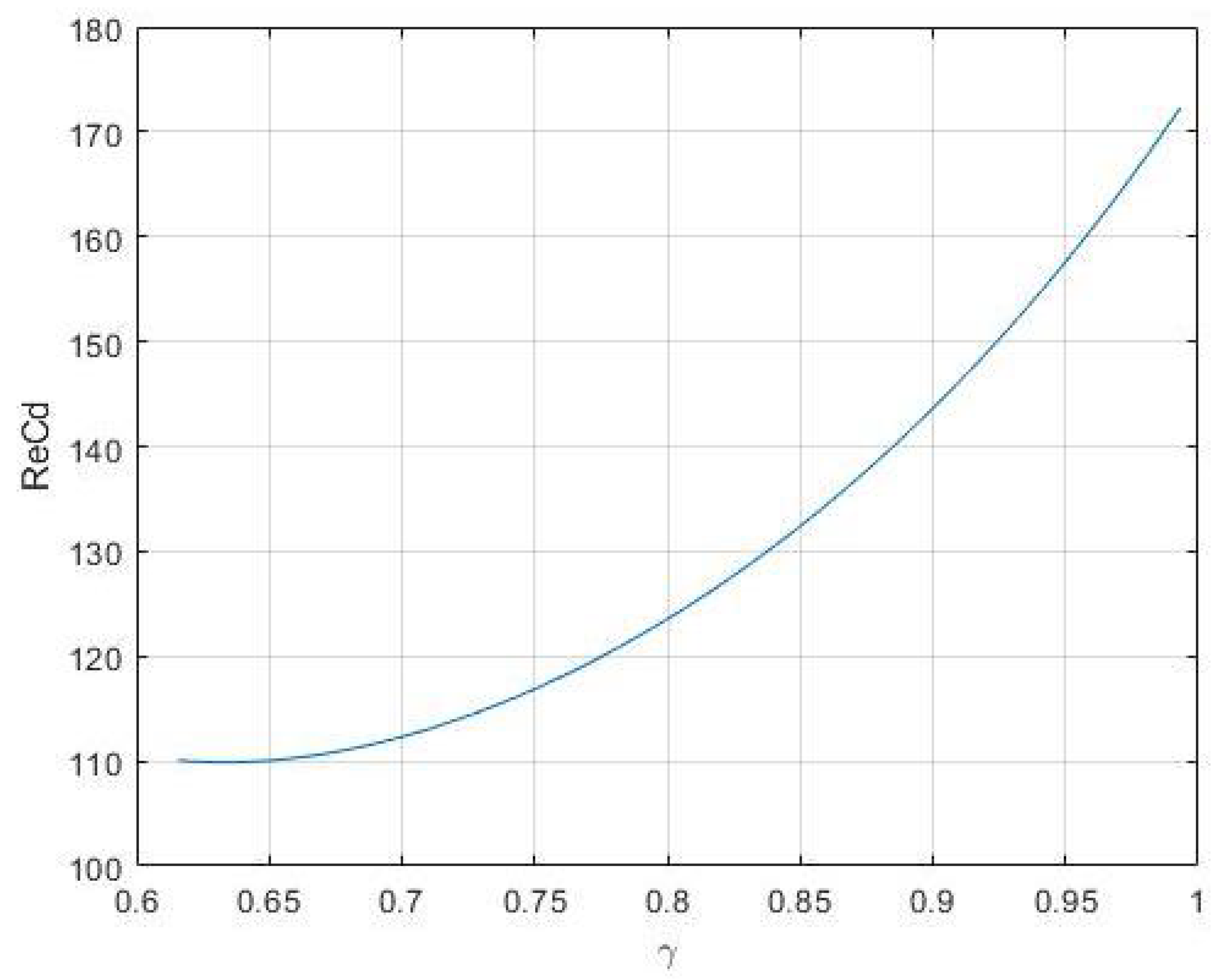
Using (8), (33), (45), and (48) we plot in Figure 11 the drag force, (the superscript (2) denotes the use of the first order approximation for the stream function, i.e., ) exerted on the solid spheroid versus the solid volume fraction of the cell, while in Figure 12 we plotted the (the superscript (2) denotes the use of the first order approximation for the stream function, i.e., ) versus the solid volume fraction of the cell, These figures are depicted using and and, therefore, Since the normal aspect ratio of an RBC [27] is we plotted the drag force and the ReCd, taking into account a deformation of the RBC from up to The aspect ratio of the cell is 4 when and
From Figure 11, we see that the drag force increases more slowly when [0.23, 0.3] and faster at higher values of . This means that, for small values of the volume fraction of the Happel cell in-cell model, the neighboring cells have a smaller effect on the flow, while when they rapidly influence the flow since the drag on the cell is much higher.
A quantitative study indicated that the stream function using only the first term of the series expansion provided satisfactory results for applications when and the moderate axis ratio of the spheroids It is observed that, as the solid volume fraction of the cell increases, both and increase and, specifically for values , the rate of the increase grows more rapidly as is shown in Figure 11 and Figure 12.
4. Conclusions
In the present manuscript, we further expanded the concept of particle-in-cell models from convex to non-convex ones and particularly to inverted spheroids, and we used this to study the flow of a swarm of erythrocytes (RBCs) into the blood plasma. The particle-in-cell model consists of two confocal inverted prolate spheroids, where the inner one represents the RBC and the exterior one stands for the boundary of the fictitious fluid envelope surrounding the RBC. In this way, we modeled the disturbance that the neighboring erythrocytes of the swarm cause to the flow. The thickness of the fluid envelope was defined so that the fluid volume fraction of the cell should be equal to the fluid volume fraction of the swarm.
Due to the physical characteristics of the blood’s flow in capillaries, the inertial non-linear terms of the Navier–Stokes equation are negligible. Furthermore, we assumed that, due to the small diameter of the capillaries, the flow is axisymmetric, which allows the reduction of the original 3D problem to an axisymmetric 3D one and, practically, to a 2D one. Moreover, the axisymmetric Stokes flow was considered to be at a steady state. This provided a very good approximation of the real problem.
The problem was fully described by a fourth order partial differential equation of elliptic type for a scalar function, i.e., where is the stream function, is the Stokes operator, and is the Stokes bistream operator. Moreover, the Happel-type boundary conditions were imposed; i.e., on the inner inverted spheroidal surface, no slip conditions were in place, while the fictitious surface was assumed to be impenetrable and free of tangential stresses. These conditions secured that the model is self-sufficient with regard to mechanical energy. Since the inverted spheroidal surface is not smooth enough to apply the given boundary conditions, and due to the complex structure of the kernel space of the Stokes fourth order partial differential operator reflected by its non-separability, the analytical solution was obtained by employing the powerful Kelvin’s inversion method and the semiseparation technique [22]. The Kelvin inversion with respect to a sphere transformed the problem at hand to an equivalent one in the prolate spheroidal coordinates.
In this system, the `new’ stream function was derived in semiseparable form through series expansions of Gegenbauer functions of the first and the second kind of even order [3]. The connecting formula between the stream function in the prolate spheroidal system with the stream function in the inverted prolate spheroidal system leads to an analytical expansion for the stream function in R-semiseparable form. These results are in agreement with all the known results in the relevant geometries.
Using the stream function expansion, the velocity field and the macroscopic pressure field were derived accordingly. Streamlines representing , based on the first term of the series expansion, were depicted, shedding light on the quantitative and qualitative characteristics of the particular kind of flow. Moreover, using the first order approximation of the stream function, quantities of bioengineering interest—the drag force and the drag coefficient —were calculated and plotted versus the solid volume fraction of the cell,
The obtained analytical results may be further used for the analytical investigation of mass transport phenomena in blood flow, such as drug delivery or as a benchmark in relative numerical models.
Author Contributions
The authors contributed equally to the writing of this paper. All authors have read and agreed to the published version of the manuscript.
Funding
This research received no external funding.
Data Availability Statement
No data were used to support this study.
Conflicts of Interest
The authors declare no conflict of interest.
References
- Suresh, S. Mechanical response of human red blood cells in health and disease: Some structure-property-function relationships. J. Mater. Res. 2006, 21, 1871–1877. [Google Scholar] [CrossRef]
- Du, E.; Qiang, Y.; Liu, J. Erythrocyte Membrane Failure by Electromechanical Stress. Appl. Sci. 2018, 8, 174. [Google Scholar] [CrossRef] [PubMed]
- Happel, J.; Brenner, H. Low Reynolds Number Hydrodynamics; Kluwer Academic Publishers: Dordrecht, The Netherlands, 1991. [Google Scholar]
- Madasu, K.P. Drag force of a porous particle moving axisymmetrically in a closed cavity of micropolar fluid. J. Appl. Math. Comput. Mech. 2019, 18, 41–51. [Google Scholar] [CrossRef]
- Faltas, M.S.; Saad, E.I. Stokes flow past an assemblage of slip eccentric spherical particle-in-cell models. Math. Meth. Appl. Sci. 2011, 34, 1594–1605. [Google Scholar] [CrossRef]
- Sherief, H.H.; Faltas, M.S.; El-Sapa, S. Interaction between two rigid spheres moving in a micropolar fluid with slip surfaces. J. Mol. Liq. 2019, 290, 111165. [Google Scholar] [CrossRef]
- Stokes, G.G. On the theories of the internal friction of fluids in motion and the equilibrium and motion of elastic solids. Trans. Camp. Philos. Soc. 1945, 8, 287–319. [Google Scholar]
- Stokes, G.G. On the Effect of the Internal Friction of Fluids on the Motion of Pendulums. Trans. Camp. Philos. Soc. 1851, 8, 8–106. [Google Scholar]
- Xu, X.; Wang, M. General complete solutions of the equations of spatial and axisymmetric Stokes flow. Quart. J. Mech. Appl. Math. 1991, 44, 537–548. [Google Scholar]
- Naghdi, P.M.; Hsu, C.S. On the representation of displacements in linear elasticity in terms of three stress functions. J. Math. Mech. 1961, 10, 233–245. [Google Scholar]
- Happel, J. Viscous flow in multiparticle systems: Slow motion of fluids relative to beds of spherical particles. AICHE J. 1958, 4, 197–201. [Google Scholar] [CrossRef]
- Kuwabara, S. The Forces experienced by Random Distributed Parallel Circular Cylinders or Spheres in a Viscous Flow at Small Reynolds Numbers. J. Phys. Soc. Jpn. 1959, 14, 527–532. [Google Scholar] [CrossRef]
- Ismailov, M.R.; Shevchuk, A.N.; Khusanov, H. Mathematical model describing erythrocyte sedimentation rate. Implications for blood viscocity changes in traumatic shock and crush syndrome. Biomed. Eng. Online 2005, 4, 24. [Google Scholar] [CrossRef]
- Cha, K.; Brown, F.E.; Wilmore, W.D. A new bioelectrical impedance method for measurement of the erythrocyte sedimentation rate. Physiol. Meas. 1994, 15, 499–508. [Google Scholar] [CrossRef]
- Datta, S.; Deo, S. Stokes flow with slip and Kuwabara boundary conditions. Proc. Indian Acad. Sci. 2002, 112, 463–475. [Google Scholar] [CrossRef]
- Madasu, K.P. Slip flow of a sphere in non-concentric spherical hypothetical cell. J. Appl. Math. Comput. Mech. 2020, 19, 59–70. [Google Scholar] [CrossRef]
- McWhirter, J.L.; Noguchi, H.; Gompper, G. Flow-Inducted Clustering and Alignment of Red Blood Cells in Microchannels. Proc. Natl. Acad. Sci. USA 2009, 106, 6039–6043. [Google Scholar] [CrossRef]
- Noguchi, H.; Gompper, G. Shape Transitions of Fluid Vesicles and Red Blood Cells in Capillary Flows. Proc. Natl. Acad. Sci. USA 2005, 102, 14159–14164. [Google Scholar] [CrossRef]
- Tsubota, K.; Wada, S.; Yamaguchi, T. Particle Method for Computer Simulation of Red Blood Cell Motion in Blood Flow. Comput. Methods Programs Biomed. 2006, 83, 139–146. [Google Scholar] [CrossRef] [PubMed]
- Bagchi, P. Mesoscale Simulation of Blood flow in Small Vessels. Biophys. J. 2007, 92, 1858–1877. [Google Scholar] [CrossRef] [PubMed]
- Dassios, G.; Hadjinicolaou, M.; Coutelieris, F.A.; Payatakes, A.C. Stokes flow in spheroidal particle-in-cell models with Happel and Kuwabara boundary conditions. Int. J. Eng. Sci. 1995, 33, 1465–1490. [Google Scholar] [CrossRef]
- Dassios, G.; Hadjinicolaou, M.; Payatakes, A.C. Generalized Eigenfunctions and Complete Semiseparable Solutions for Stokes Flow in Spheroidal Coordinates. Q. Appl. Math. 1994, 52, 157–191. [Google Scholar]
- Lebedev, N.N. Special Functions and Their Applications; Dover Publications: Mineola, NY, USA, 1972. [Google Scholar]
- Sherief, H.H.; Faltas, M.S.; Ashmawy, E.A.; Nashwan, M.G. Stokes flow of a micro-polar fluid past an assemblage of spheroidal particle-in-cell models with slip. Phys. Scr. 2015, 90, 055203. [Google Scholar] [CrossRef]
- Vafeas, P.; Protopapas, E.; Hadjinicolaou, M. On the Analytical Solution of the Kuwabara-Type Particle-in-Cell Model for the Non-Axisymmetric Spheroidal Stokes Flow via the Papkovich–Neuber Representation. Symmetry 2022, 14, 170. [Google Scholar] [CrossRef]
- Davis, J.A.; Inglis, D.W.; Morton, K.J.; Lawrence, D.A.; Huang, L.R.; Chou, S.Y.; Sturm, J.C.; Austin, R.H. Deterministic Hydrodynamics: Taking Blood Apart. Proc. Natl. Acad. Sci. USA 2003, 103, 14779–14784. [Google Scholar] [CrossRef]
- Sugii, Y.; Okuda, R.; Okamoto, K.; Madarame, H. Velocity Measurement of Both Red Blood Cells and Plasma of in vitro Blood Flow using High-Speed Micro PIV Technique. Meas. Sci. Technol. 2005, 16, 1126–1130. [Google Scholar] [CrossRef]
- Lima, R.; Ishikawa, T.; Imai, Y.; Yamaguchi, T. Blood Flow Behavior in Microchannels: Past, Current and Future Trends. Chem. Biomed. Eng. 2012, 35, 513–547. [Google Scholar]
- Dassios, G.; Hadjinicolaou, M.; Protopapas, E. Blood Plasma Flow Past a Red Blood Cell: Mathematical Modelling and Analytical Treatment. Math. Methods Appl. Sci. 2012, 35, 1547–1563. [Google Scholar] [CrossRef]
- Hadjinicolaou, M.; Kamvyssas, G.; Protopapas, E. Stokes flow applied to the sedimentation of a red blood cell. Q. Appl. Math. 2015, 73, 511–523. [Google Scholar] [CrossRef]
- Hadjinicolaou, M.; Protopapas, E. A microscale mathematical blood flow model for understanding cardiovascular diseases. Adv. Exp. Med. Biol. 2020, 1194, 373–387. [Google Scholar]
- Hadjinicolaou, M.; Protopapas, E. On the R-semiseparation of the Stokes bi-stream operator in the inverted prolate spheroidal coordinates. Math. Meth. Appl. Sci. 2014, 37, 207–211. [Google Scholar] [CrossRef]
- Moon, P.; Spencer, D.E. Field Theory Handbook; Springer: Berlin, Germany, 1961. [Google Scholar]
- Dassios, G. The Kelvin Transformation in Potential Theory and Stokes Flow. Ima J. Appl. Math. 2009, 74, 427–438. [Google Scholar] [CrossRef]
Figure 1.
Swarm of red blood cells in Stokes flow.

Figure 2.
Statement of the problem.

Figure 3.
Kelvin’s inversion.

Figure 4.
The inverted domain.

Figure 5.
.

Figure 6.
.

Figure 7.
.

Figure 8.
.

Figure 9.
.

Figure 10.
.

Figure 11.
The drag force, versus the solid volume fraction of the cell, .

Figure 12.
The drag coefficient, versus the solid volume fraction of the cell, .

Disclaimer/Publisher’s Note: The statements, opinions and data contained in all publications are solely those of the individual author(s) and contributor(s) and not of MDPI and/or the editor(s). MDPI and/or the editor(s) disclaim responsibility for any injury to people or property resulting from any ideas, methods, instructions or products referred to in the content. |
© 2023 by the authors. Licensee MDPI, Basel, Switzerland. This article is an open access article distributed under the terms and conditions of the Creative Commons Attribution (CC BY) license (https://creativecommons.org/licenses/by/4.0/).
Share and Cite
MDPI and ACS Style
Maria, H.; Protopapas, E. Non-Convex Particle-in-Cell Model for the Mathematical Study of the Microscopic Blood Flow. Mathematics 2023, 11, 2156. https://0-doi-org.brum.beds.ac.uk/10.3390/math11092156
AMA Style
Maria H, Protopapas E. Non-Convex Particle-in-Cell Model for the Mathematical Study of the Microscopic Blood Flow. Mathematics. 2023; 11(9):2156. https://0-doi-org.brum.beds.ac.uk/10.3390/math11092156
Chicago/Turabian StyleMaria, Hadjinicolaou, and Eleftherios Protopapas. 2023. "Non-Convex Particle-in-Cell Model for the Mathematical Study of the Microscopic Blood Flow" Mathematics 11, no. 9: 2156. https://0-doi-org.brum.beds.ac.uk/10.3390/math11092156
Note that from the first issue of 2016, this journal uses article numbers instead of page numbers. See further details here.