Research on Dynamic Takeout Delivery Vehicle Routing Problem under Time-Varying Subdivision Road Network

Abstract

For the dynamic takeout delivery vehicle routing problem, which faces fluctuating order demand and time-varying speeds, this study presents a novel approach. We analyze the time distribution of takeout orders and apply a Receding Horizon Control (RHC) strategy to convert the dynamic challenge into a static one. The driving speed of delivery vehicles on different roads at different times is determined based on the subdivision criteria of the urban road network and a traffic congestion measurement method. We propose a dynamic takeout delivery vehicle routing optimization model and a time-varying subdivision road network is established to minimize the total delivery cost. We validated the model through simulation examples. The optimization results show that the total distribution cost is reduced after considering the time-varying subdivision road network, with the penalty cost decreasing by 39%. It is evident that considering the subdivision of the road network can enhance order delivery efficiency and optimize the overall dining experience. The sensitivity analysis of various parameters reveals that the delivery platform must appropriately determine the time domain and allocate the number of delivery personnel based on order scale to avoid escalating delivery costs. These findings provide theoretical guidance for vehicle routing planning in the context of delivery platforms.

1. Introduction

The ‘Internet + catering’ business model is emerging with the rapid advancement of the mobile Internet and the acceleration of individuals’ pace of life. By December 2022, China’s takeout delivery user base expanded 521 million, accounting for 48.8% of the overall number of netizens. Online takeout has become an important Internet application in many people’s daily life. The generation of takeout orders occurs during peak dining hours, which often coincide with peak commuting times. The influx of a large number of individuals and vehicles on the road leads to a significant increase in traffic flow, resulting in congestion, which slows down the speed of delivery vehicles. Effectively planning delivery routes, managing traffic congestion, and ensuring prompt pick-up and delivery of takeout are pressing challenges faced by takeout platforms.

Takeout delivery is essentially a vehicle routing challenge that considers both delivery and time windows. The current research on this problem can be divided into two dimensions: static and dynamic delivery. Initially, scholars primarily focused on static research related to takeout delivery. Optimization models were constructed by considering not only the total cost of delivery but also objective functions from various perspectives. The factors to be considered included customer satisfaction [1,2,3,4,5,6], rider balance utilization [2], merchant satisfaction [5,7], and transportation efficiency [8]. Currently, in terms of algorithmic solutions, heuristic algorithms are predominantly employed by scholars, including the improved ant colony algorithm [8], fireworks algorithm [9], genetic algorithm [7,10], and adaptive large neighborhood search algorithm [11]. Several scholars have employed a combination of algorithms in their research. Zhang [3] proposed a hybrid algorithm that integrates tabu search with the water wave optimization algorithm. Zhao [12] introduced a two-stage heuristic algorithm that combines the K-means genetic algorithm with an improved variable neighborhood search algorithm. Gao [9] considered security in the delivery process. Zhao [10] considered the uncertainty of driving time. Guo [13] considered the scenarios of rider pick up and delivery crossover and picking up orders on the way. Meanwhile, scholars are investigating various takeout delivery models. Feng [4] studied a takeout delivery mode that combines two methods: riders’ independent order taking and platforms’ order dispatching. Zhao [12] considered the delivery mode of riders combined with drones. Yang [14] studied the delivery mode with the characteristics of multiple products in one order.

Due to the real-time nature of takeout order demand, it is essential to make immediate adjustments to the delivery routes when new orders are placed to effectively respond to dynamic changes in demand. Consequently, scholars have progressively directed their attention toward research on dynamic takeout delivery. At present, the solutions to this problem mainly adopt a periodic optimization strategy [15] and a continuous optimization strategy [16], which transform the dynamic problem into a static problem and solve it by combining heuristic algorithms. Yu [17] designed a rolling time-domain delay delivery algorithm, aiming to minimize the delivery distance, and constructed a vehicle routing model with hard time windows for instant delivery of O2O fresh takeout orders. Li [18] proposed a “merchant–customer” matching strategy that employs the k-means clustering method for classifying “merchant–customer” pairs and a genetic algorithm for optimizing path selection within the same category. Zhou [19] established and optimized a takeout delivery route optimization model based on business districts as the delivery center. Zhang [20] introduced the concept of customer prioritization based on different orders and developed a multi-objective O2O takeout instant delivery vehicle route planning model that considers both customer satisfaction and delivery cost. Fan [21] optimized the quality of the initial solution by clustering orders in the solving process to find solutions more quickly. Wu [22] proposed a solution for the online optimization problem of pick-up and delivery paths in distribution scenarios by considering an asymmetric network structure. Xiong [23] considered various disturbance factors that riders may encounter in the delivery process, such as temporary traffic control and abnormal delivery times of merchants and customers. Wu [24] considered the uncertainty of demand in the delivery service process and the conditions for the delivery vehicle to return to its origin for pick-up.

Delivery vehicles navigate through the urban road system, which exhibits time-varying subdivision network characteristics during the delivery process. Urban roads have a large traffic flow and many intersections, which often cause traffic congestion due to rush hour and road construction. These factors result in changes in road speed within different time periods, reflecting the typical characteristics of time-varying road networks. These characteristics affect the pick-up and delivery time of takeout food. Moreover, urban road networks can be categorized into expressways, main roads, secondary roads, and branches. The predominant delivery vehicles in these areas are electric bicycles, primarily operating on secondary roads and branches. These characteristics of the subdivision road network influence the selection of driving routes by delivery vehicles, consequently impacting pick-up and delivery times. However, the existing studies on static [1,2,3,4,5,6,7,8,9,10,11,12,13,14] and dynamic [17,18,19,20,21,22,23,24] takeout delivery have not considered the time-varying subdivision road network conditions during the driving process of takeout vehicles. Therefore, these research findings fail to adequately consider selecting optimal routes based on varying congestion levels of different roads, thereby impacting both the actual delivery time of takeout orders and customers’ dining experience.

In light of this, the present study addresses the dynamic problem of takeout delivery within a time-varying subdivision road network, investigates the influence of varying levels of road congestion on delivery time, and conducts route planning for takeout delivery vehicles. To convert the dynamic problem into a static problem across multiple time domains, this paper employs the RHC strategy [25]. Moreover, a measurement methodology is devised to determine the driving speed of takeout delivery vehicles in the context of a time-varying subdivision road network by integrating road grade and a traffic congestion coefficient. Considering the total cost encompassing the driver call cost, vehicle driving cost, and overtime delivery penalty cost, we formulate a dynamic model for optimizing takeout delivery vehicle routing with the objective of minimizing the overall expenditure.

The rest of this paper is organized as follows: In Section 2, the measurement methods of road traffic congestion degree in the subdivision road network and delivery penalty cost are designed, thus constructing the model of the takeout delivery vehicle routing problem. Section 3 introduces the overall process of model solving and designs the encoding and decoding methods of the genetic algorithm. In Section 4, experimental data are collected to build an example, solve the dynamic takeout delivery vehicle routing problem model under a time-varying subdivision road network, and analyze the solution results. Finally, we present the conclusions of our study.

2. Dynamic Takeout Delivery VRP Model

2.1. Problem Description

The service process of takeout can be broadly categorized into two stages: online order allocation and processing and offline order pickup and delivery, as illustrated in Figure 1. In the first stage, customers peruse the menu details provided by merchants and place orders via online delivery platforms. The platform then sends an application for order acceptance to the merchant. Upon confirmation by the merchant, the platform allocates the order to a rider based on its order allocation system. Simultaneously, the merchant initiates food preparation and awaits the arrival of the designated rider for food pickup. In the second stage, the rider receives this order from the platform and from the distribution center and proceeds to the corresponding merchant for food pickup. After completing the pickup, the rider adheres to a specified timeframe to deliver the food to the customer’s location, thereby accomplishing the overall comprehensive service process of this order.

Research on the takeout delivery vehicle routing problem mainly focuses on the offline pickup and delivery process of orders. After completing the order pickup, the rider starts from the distribution center and proceeds to the merchant’s location based on the order information. There, they verify the food type, quantity, and other pertinent details with the staff before completing the order pick-up process. If the merchant has not completed the food preparation at this time, the rider needs to wait for the merchant to complete this process before taking the food. Subsequently, the rider starts to deliver the orders, driving from the merchant to the corresponding customer points in the order, communicating through telephone, and delivering door-to-door. After the customer receives the takeout, the order delivery process is completed. To ensure the quality of food service, door-to-door delivery has to wait until the estimated delivery window opens, even if the rider arrives earlier. Likewise, if the rider fails to deliver within the time window, the platform has to pay a delay compensation fee to the customer.

In the process of delivery, delivery vehicles need to pass through many different roads, mainly secondary roads, and branches. These roads often face traffic congestion due to commuting, school, and other reasons, which affect delivery time. For example, in Figure 2, the rider needs to reach different merchants to pick up the food, and when the delivery vehicle encounters the school drop-off time, traffic congestion causes the vehicle speed to decrease when approaching roads near schools, which impacts the delivery time. Therefore, route planning should consider both traffic congestion and route length to ensure that delivery vehicles avoid congested roads while minimizing driving distances, thereby guaranteeing timely food delivery. The objective of this paper is to examine the impact of traffic congestion on driving speed during takeout delivery and develop a route optimization model for optimizing the performance of takeout delivery vehicles with the aim of minimizing overall costs, thereby enabling efficient planning of driving routes for such vehicles.

2.2. Solving Method

2.2.1. Dynamic Order Processing Method Based on RHC Strategy

During the actual delivery process, the demand for takeout orders exhibits real-time characteristics. The planned path must be adjusted in real time to accommodate dynamic changes in demand when new orders are generated. To incorporate the temporal distribution of takeout orders from the “China Takeout Industry Survey Report” and reduce the complexity of solving dynamic problems in real time, the RHC strategy is adopted [23]. According to the normal distribution of orders placed during the dining period, the system time is divided into equal-area time domains by definite integral, as shown in Figure 3. The newly generated orders are sequentially collected and re-planned at the end of each time domain according to their chronological order. The dynamic takeout delivery vehicle routing problem is transformed into a static one through the integration of new orders into the existing path.

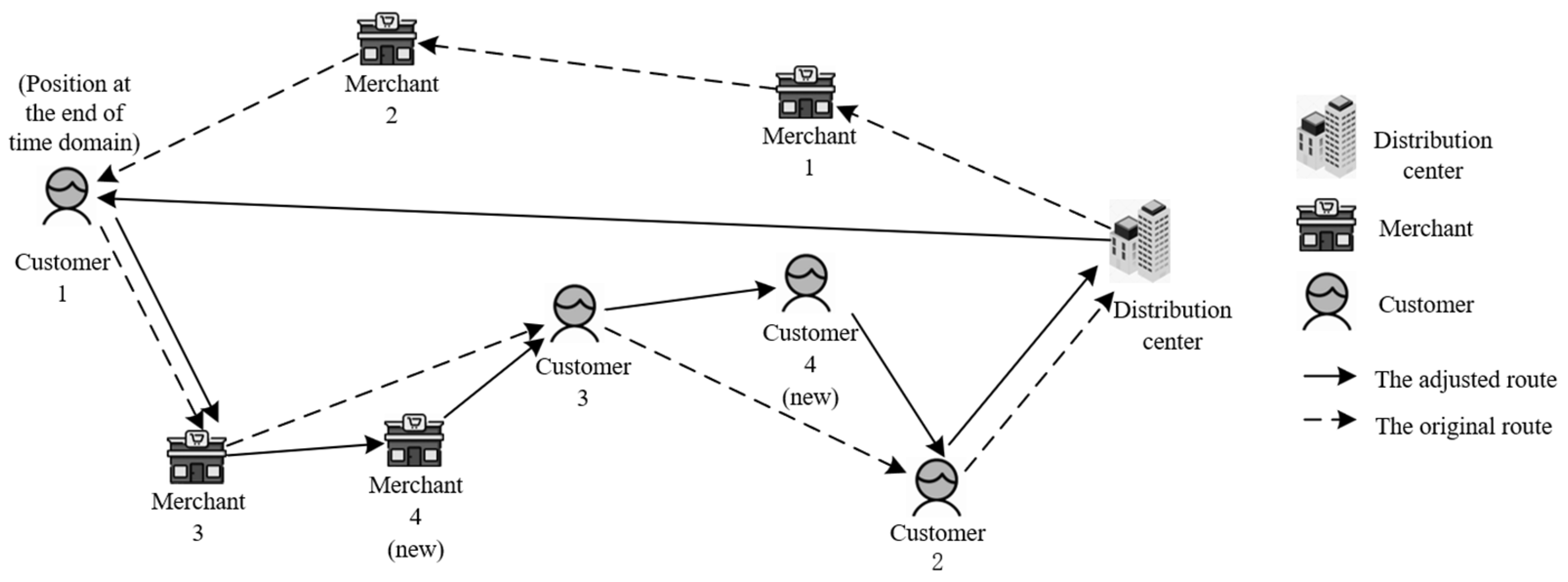
For example, the newly generated takeout order information and the node information of the takeout delivery vehicle currently located or about to arrive are collected at the end of the time domain. The time, distance, and load weight of the takeout delivery vehicle are calculated. The served node is deleted, and the takeout delivery vehicle’s current node location is the first access node to re-plan the takeout delivery path. The specific process is shown in Figure 4.

2.2.2. Measurement Methods of Road Traffic Congestion Degree in the Subdivision Road Network

(1)

Criteria for the subdivision of road networks

During the execution of delivery tasks, delivery riders are required to navigate through multiple urban roads, as depicted in Figure 5. The driving time of delivery vehicles is affected by different traffic congestion conditions on each road at different times. According to the Code for Design of Urban Road Engineering (CJJ37-2012), urban road grades are divided into four levels: expressway, main road, secondary road, and branch (

Table 1. Classification of urban roads.

Road Grade	Road Description
Express way	A central divider must be installed on urban roads with more than four motorway lanes, all or part of which adopt intersections and control access, for cars to drive at a higher speed. It is also called a car-only road. The design speed of the expressway is 60–100 km/h.
Main road	The main roads connect the various sections of the city, mainly with traffic functions. The design speed of main roads is 40–60 km/h.
Secondary road	It serves as traffic agglomeration function between the main roads and each sub-district, and it has service functions. The design speed of secondary roads is 30–50 km/h.
Branch	The connecting road between the secondary road and the neighborhood road (community road) mainly has service functions. The design speed of branches is 20–40 km/h.

).

(2)

Measurement methods for congestion degree

The delivery vehicles typically consist of electric bicycles, and their routes primarily encompass secondary and branch roads, such as the auxiliary lanes adjacent to main thoroughfares and local streets shared by motor vehicles and electric bicycles. The congestion status of secondary roads and branches is the main basis for calculating the actual driving speed of delivery vehicles. The real-time traffic query API of Baidu Map (Beijing Baidu Netcom Science Technology Co., Ltd., Beijing, China) can obtain the congestion status of secondary roads and branches at different times.

According to the “Evaluation Method for Road Traffic Congestion” (GA/T 115-2020), road traffic congestion is categorized into four levels, namely smooth, mild, moderate, and severe congestion. These levels indicate varying degrees of congestion on the road. The road experiences higher congestion and delivery vehicle speed decreases as the level increases. For the secondary and branch roads on which takeout delivery vehicles mainly drive, the designed driving speeds are 30–50 km/h and 20–40 km/h, respectively. The actual driving speed is set according to the different traffic congestion degrees in

Table 2. Driving speeds for different levels of traffic congestion under various speed limits.

Speed Limit	Average Driving Speed
	Smooth	Mild	Moderate	Severe
80	≥45	30 < $v$ ≤ 45	20 < $v$ ≤ 30	0 < $v$ ≤ 20
70	≥40	30 < $v$ ≤ 40	20 < $v$ ≤ 30	0 < $v$ ≤ 20
60	≥35	30 < $v$ ≤ 35	20 < $v$ ≤ 30	0 < $v$ ≤ 20
50	≥30	25 < $v$ ≤ 30	15 < $v$ ≤ 25	0 < $v$ ≤ 15
40	≥25	20 < $v$ ≤ 25	15 < $v$ ≤ 20	0 < $v$ ≤ 15
<40	25 < $v$ ≤ Limited	20 < $v$ ≤ 25	10 < $v$ ≤ 20	0 < $v$ ≤ 10

, which are 50 km/h and 40 km/h.

The driving speed of the delivery vehicle on the secondary road $rs$ with traffic congestion ${\theta }_{rs}(t)$ at time $t$ can thus be formulated as follows:

$$v_{rs}(t)=\{\begin{array}{cc}50-20\times {\theta }_{rs}(t)& {\theta }_{rs}(t)\in [0,1)\\ 35-5\times {\theta }_{rs}(t)& {\theta }_{rs}(t)\in [1,2)\\ 45-10\times {\theta }_{rs}(t)& {\theta }_{rs}(t)\in [2,3)\\ 60-15\times {\theta }_{rs}(t)& {\theta }_{rs}(t)\in [3,4)\end{array}$$

(1)

The driving speed on the branch road $rb$ with traffic congestion degree ${\theta }_{rb}(t)$ can be expressed as:

$$v_{rb}(t)=\{\begin{array}{cc}40-15\times {\theta }_{rb}(t)& {\theta }_{rb}(t)\in [0,1)\\ 30-5\times {\theta }_{rb}(t)& {\theta }_{rb}(t)\in [1,2)\\ 30-5\times {\theta }_{rb}(t)& {\theta }_{rb}(t)\in [2,3)\\ 60-15\times {\theta }_{rb}(t)& {\theta }_{rb}(t)\in [3,4)\end{array}$$

(2)

2.2.3. Measurement Methods of Delivery Penalty Cost

Due to traffic congestion and unreasonable delivery route planning for takeout orders, it is difficult for takeout delivery vehicles to ensure that every order can be delivered within the estimated delivery time. This study utilizes the compensation standard for overtime delivery in Meituan takeout (Beijing Science and Technology Co, Beijing, China, three fast online) as a case study. The penalty cost for overtime delivery is set equal to the actual amount of compensation provided to customers, and various penalty costs are assigned based on different levels of overtime. Assuming that the estimated delivery time window for order $o_i$ is denoted as $L{T}_i$, the actual arrival time at delivery point is represented by $A{T}_i$, and the value of the food is given as $C_i$, Equation (3) illustrates the calculation of the delivery penalty cost $p\left(A{T}_i\right)$ for this order. Additionally, Figure 6 presents a schematic diagram depicting this concept.

$$p\left(A{T}_i\right)=\{\begin{array}{cc}0& A{T}_i-L{T}_i<600\\ C_i\times 10\%& 600\le A{T}_i-L{T}_i<900\\ C_i\times 20\%& 900\le A{T}_i-L{T}_i<1800\\ C_i\times 40\%& 1800\le A{T}_i-L{T}_i\end{array}$$

(3)

2.3. Problem Description

The demand order in the process of takeout delivery exhibits real-time characteristics. Therefore, the path planning scheme needs to be dynamically adjusted with the change in the order. This paper proposes the RHC [23] strategy to address the dynamic delivery vehicle routing problem. The approach transforms the dynamic problem into a static one by considering different time domains and constructs a model by solving the static problem for each domain.

Before constructing the optimization model of takeout delivery vehicle routing, the following assumptions are made:

(1)

All delivery vehicles are of identical type and possess equivalent maximum carrying capacity;

(2)

Each delivery vehicle is paired with a rider;

(3)

The pick-up point and the delivery point in a single order are in a one-to-one correspondence, and the delivery is conducted by the same vehicle;

(4)

Upon order placement, the locations of both pick-up and delivery points, the level of demand, as well as the estimated time window for delivery are readily available;

(5)

For the same customer position in different orders, the customer is virtualized as multiple customers;

(6)

For different orders that have the same merchant location, the merchant is virtualized as multiple merchants.

From the delivery platform’s perspective, this section presents an integer programming model (4)–(19) to efficiently allocate delivery routes for each rider and ensure timely order fulfillment, with the primary objective of minimizing overall delivery costs. The symbols and parameters relevant to the model are presented in

Table 3. Symbols and related parameters in the delivery vehicle routing optimization model.

Sets
$O$	The set of takeout order numbers, $O=\left\{o_1,o_2,o_3,\dots ,o_n\right\}$, $n$ is the total number of orders.
$P^{+}$	The set of pick-up point numbers, $P^{+}=\left\{p_1,p_3,p_5,\dots ,p_{2n-1}\right\}$, $n$ is the total number of orders.
$P^{-}$	The set of delivery point numbers, $P^{-}=\left\{p_2,p_4,p_6,\dots ,p_{2n}\right\}$, $n$ is the total number of orders.
$P$	The set of all nodes, $P=p_0\cup P^{+}\cup P^{-}$, $p_0$ is the distribution center.
$RS$	Secondary road $rs\in RS$, $RS$ is the set of all secondary roads.
$RB$	Branch $rb\in RB$, $RB$ is the set of all branches.
$K$	Delivery vehicle $k\in K$, $K$ is the set of all delivery vehicles.
Parameters
${\theta }_{rs}(t)$	Traffic congestion degree of secondary road $rs$ at time $t$, $rs\in RS$.
${\theta }_{rb}(t)$	Traffic congestion degree of branch $rb$ at time $t$, $rb\in RB$.
$d_{ij}$	The distance between point $i$ and point $j$ (unit: meters), $i,j\in P$.
$d_{ij}^{rs}$	The distance traveled on secondary road $rs$ from point $i$ to point $j$ (unit: meters), $i,j\in P$, $rs\in RS$.
$d_{ij}^{rb}$	The distance traveled on branch $rb$ from point $i$ to point $j$ (unit: meters), $i,j\in P$, $rb\in RB$.
$v_{rs}(t)$	Average driving speed on secondary road $rs$ at time $t$ (unit: meters per second), $rs\in RS$.
$v_{rb}(t)$	Average driving speed on branch $rb$ at time $t$ (unit: meters per second), $rb\in RB$.
$T_{ij}^{rs}$	The driving time on secondary road $rs$ from point $i$ to point $j$ (unit: seconds), $i,j\in P$, $rs\in RS$.
$T_{ij}^{rb}$	The driving time on branch $rb$ from point $i$ to point $j$ (unit: seconds), $i,j\in P$, $rb\in RB$.
$T_{ij}$	Driving time from point $i$ to point $j$ (unit: seconds), $i,j\in P$.
$A{T}_i$	The arrival time of node $i$ (unit: seconds), $i\in P$.
$C{T}_i$	The departure time of node $i$ (unit: seconds), $i\in P$.
$R{T}_i$	For order $i$, the duration of food preparation by the merchant (unit: seconds), $i\in O$.
$E{T}_i$	For order $i$, the earliest delivery time (unit: seconds), $i\in O$.
$L{T}_i$	For order $i$, the latest delivery time (unit: seconds), $i\in O$.
$S{T}_{2i-1}$	For order $i$, service time at pick-up point $p_{2i-1}$ (unit: seconds), $i\in O$.
$S{T}_{2i}$	For order $i$, service time at delivery point $p_{2i}$ (unit: seconds), $i\in O$.
$D_{2i-1}$	For order $i$, demand for pick-up point $p_{2i-1}$ (unit: grams), $D_{2i-1}>0$, $i\in O$.
$D_{2i}$	For order $i$, demand for delivery point $p_{2i}$ (unit: grams), $D_{2i}<0$, $i\in O$.
$L_i^k$	The load of delivery vehicle $k$ at point $i$ (unit: gram), $i\in P$, $k\in K$.
$C_i$	The price of food in takeout order $i$ (Unit: RMB), $i\in O$.
$Q$	Load limit for delivery vehicle (unit: grams).
$C_1$	The cost of calling delivery vehicle (unit: RMB).
$C_2$	Cost of driving distance (unit: RMB per meter).

, while the decision variables are enumerated in

Table 4. Decision variables in the model of delivery vehicle routing optimization.

Decision Variables
$x_{ijk}$	When $x_{ijk}=1$, it means that delivery for points $i$ to $j$ is carried out by the delivery vehicle $k$, and vice versa, $i,j\in P$, $k\in K$.

.

$$MinZ=C_1\times {\displaystyle \sum _{k\in K}{\displaystyle \sum _{j\in P}{x}_{0jk}}}+C_2\times {\displaystyle \sum _{k\in K}{\displaystyle \sum _{i\in P}{\displaystyle \sum _{j\in P}{x}_{ijk}\times d_{ij}+{\displaystyle \sum _{i\in P}p\left(A{T}_i\right)}}}}$$

(4)

s.t.

$$\begin{array}{cc}{\displaystyle \sum _{k\in K}{\displaystyle \sum _{j\in P}{x}_{ijk}=1}}& \forall i\in P^{+}\end{array}$$

(5)

$${\displaystyle \sum _{k\in K}{\displaystyle \sum _{i\in P}\begin{array}{cc}{x}_{ijk}=1& \forall j\in P^{-}\end{array}}}$$

(6)

$$\begin{array}{cc}{\displaystyle \sum _{i\in P^{+}}{x}_{0ik}=1}& \forall k\in K\end{array}$$

(7)

$$\begin{array}{cc}{\displaystyle \sum _{j\in P^{-}}{x}_{j0k}=1}& \forall k\in K\end{array}$$

(8)

$$\begin{array}{cc}{\displaystyle \sum _{j\in P}{x}_{(2i-1)jk}-{\displaystyle \sum _{j\in P}{x}_{j(2i)k}=0}}& \forall i\in O,\forall k\in K\end{array}$$

(9)

$$d_{ij}={\displaystyle \sum _{rs\in RS}{d}_{ij}^{rs}+{\displaystyle \sum _{rb\in RB}{d}_{ij}^{rb}}},\forall i,j\in P,i\ne j$$

(10)

$$\begin{array}{cc}C{T}_i=\max \left(A{T}_i,R{T}_i\right)+S{T}_i& \forall i\in P^{+}\end{array}$$

(11)

$$\begin{array}{cc}C{T}_i=\max \left(A{T}_i,E{T}_i\right)+S{T}_i& \forall i\in P^{-}\end{array}$$

(12)

$$\begin{array}{cc}{T}_{ij}^{rs}=\frac{d_{ij}^{rs}}{v_{rs}(C{T}_i)}\times {\displaystyle \sum _{k\in K}{x}_{ijk}}& \forall i,j\in P \& i\ne j,\forall rs\in RS\end{array}$$

(13)

$$\begin{array}{cc}{T}_{ij}^{rb}=\frac{d_{ij}^{rb}}{v_{rb}(C{T}_i)}\times {\displaystyle \sum _{k\in K}{x}_{ijk}}& \forall i,j\in P \& i\ne j,\forall rb\in RB\end{array}$$

(14)

$$\begin{array}{cc}{T}_{ij}={\displaystyle \sum _{rs\in RS}{T}_{ij}^{rs}+{\displaystyle \sum _{rb\in RB}{T}_{ij}^{rb}}}& ,\forall i,j\in P \& i\ne j\end{array}$$

(15)

$$\begin{array}{cc}A{T}_j={\displaystyle \sum _{k\in K}{\displaystyle \sum _{i\in P}\left(C{T}_i+T_{ij}\right)\times x_{ijk}}}& \forall j\in P\end{array}$$

(16)

$$A\begin{array}{cc}{T}_{2i-1}<A{T}_{2i}& \forall i\in O\end{array}$$

(17)

$$\begin{array}{cc}{L}_j^k={\displaystyle \sum _{k\in K}{\displaystyle \sum _{i\in P}(L_i^k+D_j)\times x_{ijk}}}& \forall j\in P\end{array}$$

(18)

$$\begin{array}{cc}{L}_j^k\le Q& \forall k\in K\end{array},\forall j\in P$$

(19)

$$\begin{array}{cc}{x}_{ijk}=\left\{0,1\right\}& \forall i\in P,\forall j\in P,\forall k\in K\end{array}$$

(20)

In the takeout delivery vehicle routing optimization model, Equation (4) represents the objective function of minimizing the total cost, which encompasses the driver call cost, vehicle driving cost, and overtime delivery penalty cost. Constraints (5) and (6) ensure the fulfillment of both pick-up and delivery requirements of the order. Constraints (7) and (8) indicate that the distribution vehicle starts from the distribution center to the pick-up point and returns to the distribution center from the delivery point. Constraint (9) ensures that the same distribution vehicle services the pick-up and delivery points within the same order. Equation (10) represents the calculation formula of the distance between different nodes, which consists of the driving distance on the secondary main road and branches. Equation (11) represents the calculation formula of the time when the delivery vehicle leaves the pick-up point. Equation (12) represents the calculation formula of the time that the delivery vehicle leaves the delivery point. Equations (13) and (14) respectively represent the calculation formulas of the driving time on the secondary main road and branches when the distribution vehicle goes to the next node. Equation (15) represents the calculation formula of the driving time of the delivery vehicle between different nodes. Equation (16) is the calculation formula of the arrival time of the node. Constraint (17) ensures the principle of first take, then send. Equation (18) is the calculation formula of the load of the distribution vehicle. Constraint (19) ensures that the actual load of the vehicle is less than the maximum load limit. Equation (20) is the value range limit of the decision variable.

3. Model Solving

3.1. Overall Process

This paper presents a dynamic takeout delivery vehicle routing optimization model under the conditions of a time-varying subdivision road network, where the number of orders and status information of vehicles change constantly during the delivery process. To address this dynamic vehicle routing problem, the present study employs the RHC strategy to convert the dynamic model into multiple continuous similar static models. A heuristic algorithm is then employed to solve the static model and obtain an optimal delivery vehicle routing plan. The specific solving process is illustrated in Figure 7.

The system time is divided into multiple time domains. The new orders and rider information generated within the time domain are collected along with the unfinished service orders in the previous time domain, and the genetic algorithm is used to re-plan the delivery vehicle paths for takeout. At the end of the time domain, the unserved orders and the location of the rider are collected as the objects to be optimized and the first service point in the next time domain. Simultaneously, it is ascertained if there are any orders that have been collected but not yet delivered. If not, the next time domain is entered directly. Otherwise, the delivery point of the order must be served by the rider at the pick-up point during the optimization in the next time domain. When the last time domain route solving is complete, the dynamic solving of the takeout delivery vehicle routing problem is complete.

3.2. Algorithm Design

This section redesigns the encoding and decoding operations of chromosomes and introduces the selection, crossover, and mutation parts.

(1)

Encoding and decoding of chromosomes

To ensure that the same vehicle serves both the pick-up and delivery points of each order during the delivery process, we propose a multi-chromosome hybrid coding method based on the service node number and delivery vehicle number. Firstly, code design is conducted for the pick-up and delivery points of various orders. As illustrated in Figure 8, for order $i$, its pick-up point number is $2i-1$ and its delivery point number is $2i$.

Secondly, a chromosome of length $3n$ is generated for an individual with $n$ orders. The first $2n$ segments employ the permutation coding method to generate the access sequence of pick-up and delivery points in each order, while the remaining $n$ segments utilize the real value coding method to allocate corresponding delivery vehicles for each order. As illustrated in Figure 9, the generated chromosome corresponds to an individual characterized by 4 orders and 2 delivery vehicles. According to the node coding, the access order of each node is 7-5-8-3-1-6-2-4. According to the vehicle coding, delivery vehicle 2 is assigned to nodes 7, 8, 1, and 2, while delivery vehicle 1 is assigned to nodes 3, 4, 5, and 6. The driving order of each vehicle is determined as follows: vehicle 1: 5-3-6-4, and vehicle 2: 7-8-1-2.

(2)

The processes of selection, crossover, and mutation

Selection operation refers to selecting outstanding individuals from a population to produce the next generation of the population. This paper adopts the tournament method for selection operation. Crossover refers to the process of combining the genes of two or more individuals to generate new individuals in the evolutionary process. For the permutation encoding part, this paper adopts the partial matching crossover method, and for the real value encoding part, it adopts the two-point crossover method. Mutation refers to the random change of one or more genes in an individual’s genes to produce a new individual. For the permutation encoding part, this paper adopts the inverse mutation method, and for the real value encoding part, it adopts the breeder GA mutation method.

(3)

The enhanced elitist preservation strategy

The enhanced elitist preservation strategy refers to selecting a certain proportion of elite individuals from the current population, and directly copying them into the next generation. Then, a certain proportion of other individuals from the population are selected for crossover and mutation operations. The proposed approach ensures a certain proportion of excellent individuals in each generation, thereby enhancing the population’s convergence and global optimization capabilities.

4. Verification and Analysis

4.1. Example Construction

Taking Xi’an Bell Tower as the center and radiating 2 km to the surroundings, 50 real residential communities and 40 takeout businesses within the scope are selected as customers and merchants for the takeout orders, respectively. Their distribution is shown in Figure 10. The simulation research on takeout delivery of 50 orders within one hour during the lunch period is conducted. The order time followed a normal distribution, the food weight range of the order is 500 to 1000, the food value range is 15 to 30, the preparation time range of food is 300 to 600 after the customer places the order, the estimated delivery window for the order is 1200 to 2100 after the order is placed, and the service time range of the rider to customers and merchants is 45 to 60. Part of the takeout order information is shown in

Table 5. Part of takeout order data.

Order Number	Order Time	Food Weight (Grams)	Food Price (RMB)	Location of Pick-Up Point	Location of Delivery Point	Distance between Two Points
1	11:10:59	841	16	(34.273488, 108.952349)	(34.258614, 108.96526)	2829
2	11:24:13	986	29	(34.273384, 108.972752)	(34.25571, 108.966724)	2431
3	11:24:40	706	29	(34.248861, 108.952353)	(34.271948, 108.952094)	3698
4	11:26:26	842	28	(34.261158, 108.947717)	(34.279485, 108.945353)	2536
5	11:27:59	856	29	(34.264237, 108.970589)	(34.264009, 108.945872)	2450

.

To assess the temporal variation in driving speeds of delivery vehicles, through the traffic API of Baidu Map (Beijing Baidu Netcom Science Technology Co., Ltd., Beijing, China), we collected data on traffic congestion levels along the main routes (including secondary roads and branches) used by electric bikes within the geographical area covered by our sample of delivery orders during the lunch hour over a period of 14 days. The traffic congestion levels were converted into real-time driving speeds of delivery vehicles according to Table 2 and Equations (1) and (2). The corresponding traffic congestion levels for part of roads during various time periods are presented in

Table 6. Traffic congestion on secondary roads.

Secondary Roads	11:00	11:15	11:20	11:25	11:30
Gongnong road	1	1	1	1	1
Changying west road	2	3	3	3	2
North courtyard gate	1	1	1	2	1
Xi 1st road	1	1	3	1	1
Dongguan street	1	1	1	2	1
Cypress grove road	1	2	1	1	1

and

Table 7. Traffic congestion on branches.

Secondary Roads	11:00	11:15	11:20	11:25	11:30
Lixin street	1	1	1	2	1
Tangfang street	1	2	2	1	1
East 8th road	2	1	1	2	2
Shangde road	1	2	2	1	1
Shangqin road	2	1	1	1	1
North Guangji street	3	2	3	2	2

.

4.2. Test Simulation

This paper presents a dynamic optimization model for takeout delivery vehicles in a time-varying subdivision road network. The model is implemented using Python 3.8 and executed on a computer running the 64-bit Windows 11 operating system with 16 GB of memory and a CPU frequency of 2.3 GHz. The total duration for order generation is set to 3600 s, with a division into 6 time domains. The intervals and corresponding order numbers for each time domain are presented in

Table 8. Time intervals and generated orders.

Time Domain Interval	Orders Generated within the Interval
[0, 1221]	(1, 2, 3, 4, 5, 6, 7, 8, 9)
[1221, 1542]	(10, 11, 12, 13, 14, 15, 16, 17, 18, 19)
[1542, 1800]	(20, 21, 22, 23, 24, 25)
[1800, 2057]	(26, 27, 28, 29, 30, 31)
[2057, 2378]	(32, 33, 34, 35, 36, 37, 38, 39, 40, 41)
[2378, 3600]	(42, 43, 44, 45, 46, 47, 48, 49, 50)

. The dynamic model is transformed into a static model using the RHC strategy and then solved by the multi-chromosome genetic algorithm with enhanced elitist preservation for resolution. As the model scale expands over time, the population size is set to be 50 times the current order quantity, and the number of iterations is set to be 90 times the current order quantity. To avoid generating more and more repeated individuals in the iterative process, a large crossover and mutation probability is set for the algorithm. The crossover probability of the permutation coding part is 0.7, and the mutation probability is 0.9. The crossover probability of the real value coding part is 0.7, the mutation compression rate is 0.5, and the mutation distance gradient is 20. The actual driving routes between different nodes are obtained by combining Baidu Map API (Beijing Baidu Netcom Science Technology Co., Ltd., Beijing, China), and the optimal driving schemes of delivery vehicles in different time domains are shown in

Table 9. Optimization results of delivery vehicle routing in the first time domain.

Vehicle Number	Starting Position	Initial Load	Order Taken but Not Delivered	Traveled Route	Planning Route
1	0	0	—	—	—
2	0	0	—	—	—
3	0	0	—	—	11-3-17-4-18-9-12-10
4	0	0	—	—	—
5	0	0	—	—	1-2-15-13-7-14-16-5-8-6
6	0	0	—	—	—
7	0	0	—	—	—
8	0	0	—	—	—

,

Table 10. Optimization results of delivery vehicle routing in the second time domain.

Vehicle Number	Starting Position	Initial Load	Order Taken but Not Delivered	Traveled Route	Planning Route
1	0	0	—	—	27-33-3-4-34-15-13-16-28-14
2	0	0	—	—	—
3	11	920	12	0-11	31-9-12-10-32
4	0	0	—	—	35-36-19-20
5	2	0	—	0-1-2	17-21-37-25-26-22-18-38
6	0	0	—	—	—
7	0	0	—	—	—
8	0	0	—	—	23-29-7-24-30-5-8-6

,

Table 11. Optimization results of delivery vehicle routing in the third time domain.

Vehicle Number	Starting Position	Initial Load	Order Taken but Not Delivered	Traveled Route	Planning Route
1	27	852	28	0-27	3-4-19-43-44-28-20
2	0	0	—	—	—
3	31	1600	12, 32	0-11-31	12-41-9-42-10-32
4	35	541	36	0-35	36-13-49-47-14-50-48
5	17	548	18	0-1-2-17	39-33-15-34-40-18-16
6	0	0	—	—	—
7	0	0	—	—	45-21-37-22-46-38
8	23	750	24	0-23	25-29-7-24-30-5-8-26-6

,

Table 12. Optimization results of delivery vehicle routing in the fourth time domain.

Vehicle Number	Starting Position	Initial Load	Order Taken but Not Delivered	Traveled Route	Planning Route
1	3	1838	28, 4	0-27-3	13-4-9-14-2-10
2	0	0	—	—	—
3	12	680	32	0-11-31-12	5-43-41-44-6-42-32
4	36	0	—	0-35-36	49-47-61-55-62-50-48-56
5	39	1494	18, 40	0-1-2-17-39	15-19-40-18-16-20
6	0	0	—	—	53-21-59-54-60-22
7	45	858	46	0-45	33-34-57-37-38-46-58
8	25	1451	24, 26	0-23-25	29-7-24-30-51-8-26-52

,

Table 13. Optimization results of delivery vehicle routing in the fifth time domain.

Vehicle Number	Starting Position	Initial Load	Order Taken but Not Delivered	Traveled Route	Planning Route
1	13	2694	28, 4, 14	0-27-3-13	4-14-28-75-67-68-57-59-76-60-58
2	0	0	—	—	7-55-47-61-8-56-48-62
3	5	1386	32, 6	0-11-31-12-5	79-6-80-69-32-70
4	49	657	50	0-35-36-49	63-50-64-65-77-66-78
5	15	2225	18, 40, 16	0-1-2-17-39-15	19-40-18-16-41-20-42
6	53	594	54	0-53	21-81-54-22-9-10-82
7	33	1589	46, 34	0-45-33	37-34-71-38-72-46
8	29	2217	24, 26, 30	0-23-25-29	24-26-30-73-43-51-74-44-52

and

Table 14. Optimization results of delivery vehicle routing in the sixth time domain.

Vehicle Number	Starting Position	Initial Load	Order Taken but Not Delivered	Traveled Route	Planning Route
1	14	852	28	0-27-3-13-4-14	28-75-65-91-66-76-92-73-74
2	55	1202	8, 56	0-7-55	47-61-62-48-56-51-8-43-44-52
3	79	1901	32, 6, 80	0-11-37-12-5-79	93-6-81-80-94-59-60-82-32
4	63	1646	50, 64	0-35-36-49-63	50-64-77-83-78-84-97-98
5	19	2928	18, 40, 16, 20	0-1-2-17-39-15-19	4-16-18-87-20-95-67-96-68-88-69-70
6	21	1405	54, 22	0-53-21	85-54-22-86
7	34	1798	46, 38	0-45-33-37-34	46-9-38-41-10-42
8	24	1467	26, 30	0-23-25-29-24	26-30-89-99-90-100-57-71-72-58

and Figure 11. In these tables, “Starting position” and “Initial load” refer to the position of the delivery vehicle and its load at the start of the time domain, respectively. “Order taken but not delivered” means the set of delivery node in generated order that has been picked up but not yet delivered. “Traveled route” refers to the route that the delivery vehicle has already traveled in the previous time domain, while “Planning route” refers to the route that is planned for the delivery vehicle in the current time domain.

To assess the efficacy of the RHC strategy in addressing the dynamic takeout delivery vehicle routing problem, we compared the optimization results for takeout delivery vehicle routing in the second and third time domains, as presented in Table 10 and Table 11. In the second time domain, a total of 5 couriers are called to deliver 19 takeout orders, and in the third time domain, a total of 5 takeout orders are generated. The comparison of the optimization results of delivery vehicle routing in these two time domains shows that with an increase in orders, the addition of a new delivery vehicle (No. 7) is necessary to ensure timely delivery and minimize unnecessary penalty costs. Among the existing delivery vehicles, minimal changes are observed in routes No. 3 and No. 8, while significant modifications are evident in routes No. 1, No. 4, and No. 5. The optimization scheme for the takeout delivery vehicle path in the second time domain is no longer applicable to the third time domain; therefore, it is imperative to re-optimize the path based on the current delivery status.

4.3. Result Analysis

(1)

Comparison and analysis of solution results under different conditions

To investigate the impact of time-varying subdivision road networks on the optimization outcomes of takeout delivery routes, this study compares and analyzes the optimized results of vehicle routes for takeout delivery under both time-varying subdivision road network conditions and time-varying overall road network conditions. The average congestion level of roads in the distribution area is calculated as the overall network’s congestion level, as depicted in Figure 12. The congestion degree is converted into vehicle driving speed according to Table 2, yielding the corresponding driving speeds for the entire road network during each time period. The total cost structure in each time domain stage and its composition are calculated and compared with the results under the conditions of subdivision road network, as shown in Figure 13.

As shown in Figure 13, from time domains 1 to 6, the total number of orders also increases, which requires more delivery vehicles to be called. In order to complete the delivery, the cost of driving also increases. Due to the impact of traffic congestion, the number of orders that cannot be delivered within the expected delivery time increases, further increasing the penalty cost. In time domain 3, with the increase in congestion, the delivery vehicles considering the time-varying subdivision road network will choose the slightly longer route but the road with good congestion, so the total cost of distribution will be temporarily high. But the total cost decreases when considering the subdivision road network compared with the overall road network when all orders are delivered. Although the driving cost increases slightly, the delivery penalty cost decreases significantly, by 39%, as shown in

Table 15. Total cost and composition of takeout delivery for all orders delivered under different conditions.

	Total Cost	Driving Cost	Penalty Cost
Under time-varying subdivision network	411.94	241.74	30.2
Under time-varying overall road network	428.72	238.42	50.3

. From the analysis of the cost structure under different time domain stages, it can be found that the road congestion is smooth in the initial stage of the time domain, and the difference in total cost under the overall road network and the subdivision road network is not significant. However, in the subsequent time domains, with the increase in road congestion and order demand, under the overall road network, the vehicles still choose the shortest route for delivery, whereas in the subdivided road network, vehicles will choose smooth roads according to the traffic congestion status of different roads even though the driving distance is slightly increased, resulting in higher driving costs than in the overall road network. This ensures that orders can be delivered within the time window, reduces the delivery penalty cost, and ultimately makes the total cost under the subdivision road network less than that under the overall road network. Therefore, considering time-varying subdivision road network can reduce total costs, ensure more orders can be delivered in a timely manner, and improve customers’ dining experience.

(2)

Sensitivity analysis

To analyze the impact of allocating different numbers of delivery vehicles and different numbers of time domains on the delivery cost during optimization, experiments were conducted on different numbers of delivery vehicles and different numbers of time domains under the same conditions of takeout delivery order data. The final total costs are shown in Figure 14.

When the number of time domains is fixed at six and the total number of orders is fixed at 50, the total cost of delivery shows a trend of first decreasing and then increasing with the increase in the number of delivery vehicles. This is because when the number of delivery vehicles is extremely low, the number of orders that each vehicle needs to deliver is large, and it is difficult to ensure that all orders can be delivered within the time window, resulting in high penalty costs. With the increase in the number of delivery vehicles, there is a gradual alleviation of delivery pressure on vehicles, ensuring timely delivery for most orders and minimizing the overall cost when employing eight delivery vehicles. However, beyond a certain threshold, the cost of calling delivery vehicle increases significantly, resulting in an increase in the total cost instead of a decrease. Therefore, to effectively reduce the delivery cost, it is imperative to appropriately allocate the number of delivery vehicles based on the order size when optimizing dynamic vehicle routing within a time-varying subdivision road network.

When the number of delivery personnel is fixed at eight and the total number of orders is fixed at 50, the total cost of distribution further reduces with the increase of the number of time domains, as the number of orders in each time domain decreases and the number of re-optimizations using the RHC strategy increases, leading to a better delivery scheme. Notably, this reduction is most pronounced when there are six time domains. However, frequent operations also increase the running time of the algorithm, making it difficult to guarantee a timely solution in the time domain. Therefore, to ensure timely solutions and reduce delivery costs, it is imperative to appropriately determine the number of time domains based on the optimization duration when optimizing dynamic vehicle routing within a time-varying subdivision road network.

5. Conclusions

This paper examines the impact of traffic congestion on vehicle routes during takeout delivery, considering different times and levels of roads. A dynamic optimization model for takeout delivery vehicle routes is developed based on a time-varying subdivision road network. The model is solved by the genetic algorithm in each time domain, resulting in an optimal delivery scheme for takeout vehicles. The optimization results for takeout delivery vehicle routing under a time-varying subdivision road network and a time-varying overall road network are compared and analyzed. It is found that the total cost of the time-varying subdivision road network scheme is decreased, with a significant reduction in penalty costs by 39%. Using a time-varying subdivision road network decreases overdue orders and enhances customers’ dining experience.

The solution results of route optimization are also influenced by the allocation of different numbers of delivery vehicles and the number of time domains. If the allocation of distribution vehicles is insufficient, it results in excessive distribution pressure, leading to increased penalty costs. Conversely, an excessive allocation of distribution vehicles will escalate driver call cost and consequently raise the total cost. If the number of time domains is small, it results in reduced solution accuracy; conversely, a larger number of time domains leads to increased algorithm operating time, making it difficult to guarantee timely solutions in the time domain. Therefore, it is imperative to appropriately allocate the number of delivery vehicles based on order size and determine the number of time domains based on the optimization duration, ensuring a minimized total cost.

In the actual process of takeout delivery, in addition to traffic congestion, weather conditions, order cancellations, and vehicle failures can also affect the delivery of takeout orders. Therefore, in future research, these factors can be considered to make the optimized results more realistic.

References

- Chen, P.; Li, H. Optimization Model and Algorithm based on Time Satisfaction for O2O Food Delivery. Chin. J. Manag. Sci. 2016, 24, 170–176. [Google Scholar]
- Liao, W.; Zhang, L.; Wei, Z. Multi-objective green meal delivery routing problem based on a two-stage solution strategy. J. Clean. Prod. 2020, 258, 120627. [Google Scholar] [CrossRef]
- Zhang, M.; Wu, J.; Wu, X. Hybrid evolutionary optimization for takeaway order selection and delivery path planning utilizing habit data. Complex Intell. Syst. 2021, 8, 4425–4440. [Google Scholar] [CrossRef]
- Feng, A.; Zhou, Y.; Gong, Y. Research on Takeout Distribution based on the Combination Mode of Order Dispatching and Grabbing. Control Decis. 2023, 38, 1–8. [Google Scholar]
- Wei, Z.; Li, M. Takeaway Delivery Route Optimization Considering Double Satisfaction. Logist. Eng. Manag. 2024, 46, 54–57. [Google Scholar]
- Yang, A. Research on Takeaway Distribution Path under Multiple Constraints. Int. Core J. Eng. 2020, 6, 204–208. [Google Scholar] [CrossRef]
- Ren, T.; Xu, H.; Jin, K. Optimisation of takeaway delivery routes considering the mutual satisfactions of merchants and customers. Comput. Ind. Eng. 2021, 162, 107728. [Google Scholar]
- Jin, Z.; Ju, X.; Guo, J.; Yang, Z. Optimization on distribution routes of the takeaway delivery staff under the O2O mode. J. Dalian Marit. Univ. 2019, 4, 55–64. [Google Scholar]
- Gao, W.; Jiang, G. The research based on the path optimization problem of takeaway delivery. Inf. Commun. 2018, 5e, 20–22. [Google Scholar]
- Zhao, X.; Xing, L.; Jin, Z. Bi-objective takeaway distribution route optimization considering uncertain driving time. J. Dalian Marit. Univ. 2019, 45, 65–72. [Google Scholar]
- Xu, Q.; Xiong, J.; Yang, Z. Route Optimization of Takeout Delivery Vehicles Based on Adaptive Large Neighborhood Search Algorithm. Ind. Eng. Manag. 2021, 26, 115–122. [Google Scholar]
- Zhao, Q.; Lu, F.; Wang, L. Research on Drones and Riders Joint Take-Out Delivery Routing Problem. Comput. Eng. Appl. 2022, 58, 269–278. [Google Scholar]
- Guo, H.; Xiong, H.; Ren, R. The Optimization of Takeout Delivery Route that Allows Cross Picking and Delivery and Order Halfway. Syst. Eng. 2022, 40, 70–81. [Google Scholar]
- Yang, H.; Gao, j.; Shao, E. Vehicle Routing Problem with Time Window of Takeaway Food Considering One-order-multi-product Order Delivery. Comput. Sci. 2022, 49, 191–198. [Google Scholar]
- Li, Y.; Fan, H.; Zhang, X. A Periodic Optimization Model and Solution for Capacitated Vehicle Routing Problem with Dynamic Requests. Chin. J. Manag. Sci. 2022, 8, 254–266. [Google Scholar]
- Yan, F.; Deng, D.; Chai, F.; Ma, Y. Optimization of Dynamic Collection Route of Smart Garbage Bins Considering Negative Environmental Effects. J. Transp. Syst. Eng. Inf. Technol. 2023, 23, 265–274. [Google Scholar]
- Yu, H.; Tang, W.; Wu, T. Vehicle Routing Problem with Hard Time Windows for Instant Delivery of O2O Fresh Takeout Orders. J. Syst. Manag. 2021, 30, 584–591. [Google Scholar]
- Li, T.; Lyu, X.; Li, F.; Chen, Y. Routing optimization model and algorithm for takeout distribution with multiple fuzzy variables under dynamics demand. Control Decis. 2019, 34, 406–413. [Google Scholar]
- Zhou, C.; Lyu, B.; Zhou, H. Optimization model and algorithm for Online to Offline dynamic take-out delivery routing problem centered on business districts. Oper. Res. Trans. 2022, 26, 17–30. [Google Scholar]
- Zhang, L.; Zhang, J.; Xiao, B. Multi-objective O2O Take-Out Instant Delivery Routing Optimization Considering Customer Priority. Ind. Eng. Manag. 2021, 26, 196–204. [Google Scholar]
- Fan, H.; Tian, P.; Lyu, Y.; Zhang, Y. Vehicle Routing Problem with Simultaneous Delivery and Pickup Considering Temporal-Spatial Distance in Time-Dependent Road Network. J. Syst. Manag. 2022, 31, 16–26. [Google Scholar]
- Wu, T.; Zhang, J.; Yu, H. The Real-time Pick-up and Delivery Problem with the Asymmetric Network. Chin. J. Manag. Sci. 2023, 31, 214–221. [Google Scholar]
- Xiong, H.; Guo, H.; Yan, H. Research on Real-time Route Optimization of Takeaway Delivery Considering Pickup and Delivery Cross and Multiple Disturbance Factors. J. Hunan Univ. 2022, 49, 92–102. [Google Scholar]
- Wu, T.; Chen, J.; Jian, J. The online pick-up and delivery routing problem under O2O delivery. Syst. Eng.-Theory Pract. 2018, 38, 2885–2891. [Google Scholar]
- Zhan, Y.; Ye, L.; Zheng, J. Optimization of Dynamic Takeaway Distribution Problem Based on Receding Horizon Control. Comput. Technol. Dev. 2019, 29, 83–88, 94. [Google Scholar]
Figure 1.
The overall process of food delivery.
Figure 2.
The scheme for takeout delivery route planning under various conditions.
Figure 3.
RHC strategy for dynamic takeout orders.
Figure 4.
Readjustment of the delivery route.
Figure 5.
Driving paths of takeout delivery vehicles in subdivided road network.
Figure 6.
Delivery penalty cost function.
Figure 7.
Flowchart of using the RHC strategy and genetic algorithm.
Figure 8.
The correspondence diagram between orders and pick-up and delivery points.
Figure 9.
Schematic diagram of chromosome coding.
Figure 10.
Geographical location map of merchants and customers.
Figure 11.
Optimal driving route of takeout delivery vehicles in different time domains. (a) Takeout delivery route in the first time domain. (b) Takeout delivery route in the second time domain. (c) Takeout delivery route in the third time domain. (d) Takeout delivery route in the fourth time domain. (e) Takeout delivery route in the fifth time domain. (f) Takeout delivery route in the sixth time domain.
Figure 12.
Traffic congestion degree of the overall road network at different times.
Figure 13.
Cost structure in different time domain.
Figure 14.
Total cost under different conditions. (a) Total cost under different numbers of delivery vehicles. (b) Total cost under different numbers of time domains.