Memory-Based Evolutionary Algorithms for Nonlinear and Stochastic Programming Problems


1
Department of Computer Science in Jamoum, Umm Al-Qura University, Makkah 25371, Saudi Arabia
2
Department of Computer Science, Faculty of Comp. & Info, Assiut University, Assiut 71526, Egypt
3
Department of Mathematics, Faculty of Science, Assiut University, Assiut 71516, Egypt
4
Computers and Systems Engineering Department, Mansoura University, Mansoura 35516, Egypt
*
Author to whom correspondence should be addressed.
Mathematics 2019, 7(11), 1126; https://0-doi-org.brum.beds.ac.uk/10.3390/math7111126
Submission received: 18 September 2019
/
Revised: 6 November 2019
/
Accepted: 7 November 2019
/
Published: 17 November 2019
(This article belongs to the Special Issue Evolutionary Computation and Mathematical Programming)
Abstract
:In this paper, we target the problems of finding a global minimum of nonlinear and stochastic programming problems. To solve this type of problem, we propose new approaches based on combining direct search methods with Evolution Strategies (ESs) and Scatter Search (SS) metaheuristics approaches. First, we suggest new designs of ESs and SS with a memory-based element called Gene Matrix (GM) to deal with those type of problems. These methods are called Directed Evolution Strategies (DES) and Directed Scatter Search (DSS), respectively, and they are able to search for a global minima. Moreover, a faster convergence can be achieved by accelerating the evolutionary search process using GM, and in the final stage we apply the Nelder-Mead algorithm to find the global minimum from the solutions found so far. Then, the variable-sample method is invoked in the DES and DSS to compose new stochastic programming techniques. Extensive numerical experiments have been applied on some well-known functions to test the performance of the proposed methods.
1. Introduction
In the real world, there are many challenging applications which naturally require involving optimization techniques to have the best configurations, and find the optimal resources [1]. In particular, these complex application problems are computationally expensive in a sense of resources and time and most of them contain noise. Furthermore, the objective functions associated with most of these problems are not differentiable and have a large scale of parameters. Therefore, trials to compute the derivatives using finite differences methods mostly fail.
Typically, such real complex systems are usually modeled using a series of simulation procedures to evaluate their output responses. Also, they are integrated with an optimization algorithm to find their optimal parameters. The integration of the stochastic optimization methods into simulation software packages to meet their design requirements is crucial. Thus, these techniques are called Simulation-Based Optimization (SBO) [2,3]. SBO consists of three components, design tools, precise soft simulators, and optimization techniques. There are many engineering fields using the SBO, such as aerospace [4,5,6], automotive [7,8], transportation [9], and naval [10]. One of the most difficult issue of such systems is that the objective function usually contain noise and the user should carry out several simulations to obtain an acceptable approximate value of the objective function at a single point [11]. Therefore, this research focuses on optimizing objective functions with high noise which is known as stochastic programming [12].
Usually, the term “Simulation-Based Optimization” is more common than “stochastic optimization” [11,13]. Highly non-linear and/or high dimensional real-world optimization problems require the SBO, since these problems involve uncertainties in the form of randomness. This problem is known as stochastic programming problem where the estimation of the uncertainty is carried out as a stochastic probability function. The considered problem is represented mathematically as follows:
where is the search space and f is a function with decision variables , and is the probability function of a random variable . The configuration of the simulation parameters to enhance the operation is the main challenge. Typically, the simulation process is complex, since the evaluation of its objective function is computationally expensive, the results are noisy, and the objective function does not have an exact gradient. Usually, these problems have multiple local optima, which prevents classical nonlinear programming techniques from solving such problems successfully all the time. Therefore, global search methods are the best candidates to solve these problems which can defined in the following nonlinear programming problem:
where is the search space and f is a nonlinear function with decision variables . Therefore, this research aims to design new methods to deal with Problems (1) and (2).
Recently the metaheuristics techniques, such as Evolution Strategies (ESs) and Scatter Search (SS), can solve Problem (2) by applying intelligent and learned procedures [14,15,16,17]. Metaheuristics are powerful tools since they are robust and can fight to successfully find accurate solutions of a wide range of problem areas [14,17]. However, applying the metaheuristics for complex problems converges slowly since exploring the global search space is a stochastic process that needs a high computational cost. Additionally, they usually could not remark promising search directions utilizing local information. On the other hand, the convergence of local search methods is faster since they create mathematical or logical movements based on the local information to determine promising search directions. However, they can be easily entrapped in local minima.
Typically, numerical global optimization methods are classified into deterministic, stochastic (heuristic), and hybrid techniques [18,19]. Generally, deterministic methods solve problems that are formulated based on their analytical properties, and some theoretical assumptions. Also, when there is available prior information about the problem under investigation, Branch-and-Bound algorithms in the deterministic global optimization are the most capable methods for searching the global minima [20]. The deterministic methods can find a global minimum with a pre-defined tolerance in case of having exact computation over long run time. In this type of optimization, the range of all variables defines the search space. Besides, these methods are characterized by having a theoretical assurance of finding the global solution. This means the value of the objective function when applying a local optimum differs just by small value from the global one. Old deterministic algorithms suffer from some limitations such as loose bounds, and they cannot deal with practical problems with more than ten variables. However, some new deterministic methods have been improved to obtain good results, such as the Hit-and-Run method. Also, it is modified to deal with high dimensional problems such as the Molecular Distance Geometry Problem (MDGP) instances [21], but it consumes high computational time. These limitations of the deterministic methods have motivated the transition to the stochastic methods.
On the other hand, some of stochastic methods are characterized by a probabilistic convergence guarantee, which usually means the probability of its global solution is one within infinite time. Furthermore, the stochastic methods search for the optimal solution of problems that have black-box formulations, awful behavior, and noisy evaluation functions [22]. The stochastic methods are the best candidate to search for optimal solutions when objective functions suffer from a deficiency of prior suppositions. These methods work by sampling the search space randomly. There are many techniques classified as stochastic methods such as Genetic Algorithms (GA), Simulated Annealing (SA), Tabu Search (TS), Particle Swarm Optimization (PSO), and others [23]. Typically, the stochastic search is a multistage method which consists of global and local stages. The performance of these two stages significantly affects the efficiency of the stochastic methods, which also subject to the quality of sampled points.
Each technique in the above two categories has certain advantages and drawbacks. Researchers have hybridized these techniques to enhance their performance, and make it faster and more robust [24,25]. An effective introduction to hybrid metaheuristic methods is explained in [26]. An example for these hybrid algorithm is proposed in [27], where an approximation algorithm and linear relaxations can be integrated with an ant colony-like algorithm to get a very effective and fast algorithm for multi-period capacity and routing path planning in network design. Another example of work which combines genetic algorithms with individual Quasi-Newton learning for global optimizations is shown in [28].
The considered stochastic problem is conquered by several optimizations and search techniques, such as the Variable-Sample methods (VS) [29]. These methods are classified as Monte-Carlo methods that convert unconstrained stochastic optimization problems to deterministic problems. Explicitly, an estimation of the sample performance measure containing the random variable is carried out using several sample points. The VS method is invoked by a random search algorithm called Sampling Pure Random Search (SPRS) where an average approximation method with a variable-sample size replaces the objective function in each iteration [29].
In this paper, we find the global solution of the stochastic programming problem by developing new hybrid methods combining metaheuristics techniques, such as Evolution Strategies, Scatter Search, direct search, and Variable-Sample (VS) methods. Uncertainties formed as randomness and high dimensional are the main difficulties associated with such stochastic programming problems. Two main steps are representing the proposed methods as follows:
- First, new versions of ES and SS are proposed to enhance their performance in finding the solutions of the global optimization problem defined as Problem (2):
- –
- A new version of ESs called Direct Evolution Strategy (DES) [30] is applied. The DES method is composed by integrating the ESs with a new philosophy for applying the evolution process. Specifically, reproducing offspring in the DES method has two directions. The first one is to modify the mutation operation of ESs to reproduce offspring in a closed environment of their parents and use the parents’ experience to direct the offspring towards promising directions. The other direction of reproducing offspring is achieved by modifying the recombination operation to reproduce offspring in a promising area slightly away from their parents’ environment. This offspring has exploration duties that keep the diversity of its generation and the successive ones. This process of exploration is known in the literature as “Dispersal”, which means the movement of organisms away from their point of origin [31]. More elements have been added in the DES method to achieve more diversification process and to overcome the drawback of ESs termination.
- –
- A new SS method is proposed by extending the regular SS method built based on Laguna and Martı [32] and Duarte et al. [33] and integrating it with the Gene Matrix (GM). The proposed method is called Directed Scatter Search (DSS). Particularly, a hybrid technique is applied to update the reference set of the SS, where the possible values of each variable are divided into sub-ranges stored in the GM [34]. The GM enhances the exploration process after applying a mutagenesis operator [34] by adding new diverse solutions to the search space. Mutagenesis operator works on accelerating the exploration process by altering some survival solutions.
- Second, the proposed metaheuristics techniques are combined with the Variable-Sample method to solve the simulation-based optimization problem defined as Problem (1):
- –
- The DES for Stochastic Programming (DESSP) method consists of a modified version of evolution strategies, and Monte-Carlo-based Variable-Sample technique to estimate the objective function values. The DESSP method tries to solve the stochastic global optimization problem. This problem has been considered in both cases as local and global problems.
- –
- A new method for dealing with the stochastic global optimization problem 1 is proposed. This method, called the Directed Scatter Search for Stochastic Programming (DSSSP), is an integration between the proposed SS method and the VS method. The DSSSP has two components. The Monte-Carlo-based variable-sample method is the first component that estimates the values of the objective function, while the DSS method is the second one generating solutions and exploring the search space.
The details of the proposed non-linear programming techniques and its main components are explained in Section 2 and Section 3. The variable sample methods are highlighted in Section 4. The proposed simulation-based optimization methods are introduced in Section 5 and Section 6. Section 7 explains the main numerical experiments and how the parameters of the proposed methods are selected and tuned. Finally, the conclusion is presented in Section 8.
2. Directed Evolution Strategies
Hereafter, we explain how the ESs method is modified to produce the Directed Evolution Strategies (DES) [30]. Then, the DES method is combined with a variable-sample technique to compose a simulation-based optimization method. Next, we mention some remarks about the ESs which considered as initiatives for building the DES.
In the -ES, all parents are discarded during the selection process, whether they are good or bad since a strict Darwinian selection is the approved selection mechanism. This selection mechanism is not the optimal one since we lose some good solutions when discarding all of them. On the other hand, the -ES applies different selection mechanism where the next generation only takes which are the best individuals come from the parents and offspring. This type of selection may lead to immature convergence without guarantee diversity. Therefore, a new operation called “mutagenesis” is proposed. To maintain the diversity, the proposed mutagenesis alters some survival individuals to new unexplored areas. Besides, this new operation maintains the elitism works since it works within the “+” selection mechanism.
The ESs have an unbiased chance of reproducing children, which makes them are not like genetic algorithms (GAs). During recombination and mutation operations, there is an equal chance for all parents to reproduce children. Beside, the fittest works only during the selection operation. Moreover, the recombination operation in the standard ESs has a variable number of mated parents, i.e., it supports the multi-parents recombination.
Since intelligent exploitation and exploration processes should be implemented in a good global search method, and since ESs have their promising mutation operation as an exploitation process, it is advisable to utilize a recombination mechanism which can serve as an intelligent exploration process. According to this concept, the recombination operation in the DES method has been constructed to diverse the search process towards new unexplored areas.
Another drawback in the ESs and EAs is termination criteria since there are no automatic termination criteria. In fact, in an early stage of the search process, the EAs may reach an optimal or near-optimal solution; however they could not terminate because they were not learned enough. Therefore, through successive generations, our proposed DES has termination measures to check the progress of the exploration process. Afterwards, to converge faster an exploitation process refines the best candidates obtained so far.
The remarks mentioned above have been taken into consideration while designing the proposed DES. Next explained components are integrated into the standard ESs algorithm to create the new DES method.
- Gene Matrix and Termination. During the search process, GM [34] is applied to ensure the exploration of the search space. In the GM, each variable is divided to sub-ranges based on its possible values. In the real-coding representation, there are n variables or genes in each individual x in the search space. The GM checks the diversity by dividing the range of each gene to m sub-ranges. Initially, a zero matrix of size the represents the GM where each element in each row denotes a sub-range of the equivalent gene. During the search process, GM’s values are altered from zeros to ones. An example of GM in a two-dimension search space is shown in Figure 1. We achieve an advanced exploration process when the GM has all ones. But the search will widely explore the recently chosen sub-ranges with the help of recombination operation. Therefore, the advantages of the GM are the practical termination criteria and providing the search with diverse solutions as explained hereafter.
- Mutagenesis. For accelerating the exploration process, the worst individuals selected for the next generation are reformed by a more artificial mutation operation called “mutagenesis”. Explicitly, a random zero-position in GM is selected. This will explore the j-th partition of the variable range which has not been visited yet. Then, one of the selected individuals for mutagenesis will be changed by a random value for within this partition. The formal mutagenesis procedure is explained as follows in Algorithm 1:
Algorithm 1Mutagenesis 1: procedure Mutagenesis(x, )
2: if GM is not full then
3: .
4: , where are the lower and upper bound of the variable , respectively, and r is a random number from .
5: Update .
6: else
7: Return
8: end if
9: end procedure - Recombination. The recombination operation is not applied for all parents, but with probability , since it has an exploration tendency. Initially, parents will be randomly chosen from the current generation. The number of the partitions of each recombined child equals () where partitions are taken from parents. Figure 2 displays an instant of 4 parents , , , and partitioned at the same positions into 4 partitions. Next, a recombined child is created by inheriting its four partitions from , , and , respectively. The DES recombination operation is described in Algorithm 2.
Algorithm 2Recombination - 1:
- procedureRecombination(, …, )
- 2:
- if then
- 3:
- .
- 4:
- .
- 5:
- Compose a new child .
- 6:
- else
- 7:
- Return
- 8:
- end if
- 9:
- end procedure
It is important to mention that the DES recombination procedure, defined to support the DES exploration process, is built as a standard type of the “single point crossover” and “two point crossover” [37]. Specifically in the high dimensional problems, the GM overcomes the complexity of such problem by not saving the information of the diverse sub-ranges of separate variables. Hence, as shown in the example in Figure 3a, it is possible to have misguided termination of the exploration process. However, this drawback, shown in Figure 3b, can be easily overcome by calling such recombination operation as in Algorithm 2. - Selection. The same standard ESs “+” selection operation is applied for the DES to choose from some survival individuals and insert it into its next . Though, to ensure diversity, the mutagenesis operator alters some of these individuals.
- Intensification Process. After having all children, DES applies a local search starting from two characteristic children to improve themselves. These two children are the one with the best computed solution till now, and the other child is chosen after computing the objective function of each parent and his child and select the child with the highest difference in the current generation. Therefore, these characteristic are called children “the best child” and “the most promising child” respectively. The DES behaves like a “Memetic Algorithm” [38] after applying this intensification process which accelerates the convergence [39,40]. For more intensification to enhance the best solutions found so far, we apply derivative-free local search method as an efficient local search method. At the last stage, this intensification process can enhance convergence of EAs and prevent the EAs roaming around the global solution.
Figure 4 shows the main steps of the DES method while its algorithm is explained as follows (Algorithm 3):
| Algorithm 3 DES Algorithm |
| 1: Initial Population. Set the population parameters and and calculate . Generate an initial population 2: Initial Parameters. Select the recombination probability , and set values of , , m and . Set the gene matrix GM to be an empty matrix of size . 3: Initialize the generation counter 4: while the termination conditions are not met do 5: for do 6: Recombination. Choose a random number 7: if then 8: Select a parent from . 9: else 10: Select parents from . 11: Compute the recombined child using Recombination Procedure (Algorithm 2). 12: end if 13: Mutation. Use Equations (3) and (4) to compute a mutated children . 14: Fitness. Evaluate the fitness function . 15: end for 16: Children Pool. Set to contain all children. 17: Selection. Set the next generation to contain the best individuals from . 18: Mutagenesis. Use Mutagenesis Procedure (Algorithm 1) to alter the worst solutions in 19: Update the gene matrix GM. 20: Set . 21: end while 22: Intensification. Refine the best solutions using local search. |
3. Scatter Search with Gene Matrix
Hereafter, we explain the integration between the Gene Matrix (GM) explained in Section 2, and the standard Scatter Search (SS) to compose the DSS method. The proposed DSS method involves the same five steps of the SS as follows:
- 1.
- Diversification Generation: Generating diverse trial solutions.
- 2.
- Improvement: Applying local search to improve these trial solutions.
- 3.
- Reference Set Update: Updating the reference set containing the b best solutions found. the Solutions are classified based on the quality or the diversity.
- 4.
- Solution Subset Generation: Dividing the reference set solutions into subsets to create combined solutions.
- 5.
- Solution Combination: Combining solutions in the obtained subsets to create new trial solutions.
In step 3, the Reference Set (RefSet) in the proposed DSS has three parts. These parts are updated to keep the elitism, the diversity, while the GM and mutagenesis concepts [34] explained in Section 2 are applied to update the last part. The indicator of attaining an advanced exploration process is having GM full by ones. Therefore, GM assists the diversification process by supplying the search with diverse solutions using the mutagenesis operator (Algorithm 1), and it is used as a practical termination criteria.
3.1. Updating the Reference Set
In the basic procedure of SS based on the evaluation of the objective function, a solution with high value replaces the one with the worst value for updating the reference set.
Also, another part in the RefSet is kept preserving the solution diversity [32]. The standard update procedure in the SS is a reformed technique called the Update with Gene Matrix (UpGM) in the proposed DSS method. This new update technique increases the diversity, the exploration, and exploitation processes. All solutions from the combination ones already in the RefSet make up the new offspring Pool, i.e., . Algorithm 4 represents the formal steps for the process of updating the RefSet.
| Algorithm 4Update with GM |
|
3.2. Diversity Control
In the standard SS to avoid trapping in local minima, the reference set has to be checked to circumvent duplicate solutions. However, applying this method cannot guarantee the diversity of the superior solutions while initializing the RefSet. Instead, a strict diversity check using the max-min criterion is applied to ensure the diversity of the solutions. In the initial RefSet, the chosen solutions can be exposed to a minimum diversity test as follows: The best solutions in the initial population P are chosen to be in the RefSet. Afterwards, is removed from P, and the next high-quality solution x in P is selected and added to the reference set only if it is far from . Therefore, the minimum distance between the current solutions in RefSet and the selected solution x controls the process of adding the next best solution in P at each step. This distance has to be at least as large as the threshold value to add this best solution.
3.3. DSS Algorithm
The main steps of the DSS method are shown in Figure 5 while it is formalized as described in the following Algorithm 5.
| Algorithm 5DSS Algorithm |
| 1: . 2: repeat 3: Generate a solution x using the Diversification Generation Method. 4: if ( || is not close to any member in P) then, 5: . 6: end if 7: until the size of P is equal to . 8: Compute the fitness values for all members in P. 9: Apply Update with GM Procedure (Algorithm 4) to generate an initial RefSet. 10: while the stopping criteria are not met do 11: Use the Subset Generation Method to create solution subsets of size two. 12: Generate the offspring using the Combination Method. 13: Refine the offspring using the Improvement Method and add them to Set. 14: Use the Update with GM Procedure (Algorithm 4) to update the RefSet. 15: end while 16: Refine the best solutions using a local search method. |
In this method, we apply “fminsearch.m” which is a MATLAB function implementing the Nelder-Mead method. This function improves the intensification of the proposed method (Step 16 of Algorithm 5). In the experimental work, the maximum evaluations number of the objective function is used to terminate the search process.
4. Variable Sample Method
The Variable-Sample (VS) method is classified as a class of Monte-Carlo methods for dealing with unconstrained stochastic optimization problems. The stochastic optimization problem can be converted using the VS to a deterministic problem, where an estimation of the sample performance measure containing the random variable is carried out using several sample points. The VS method is usually called by the Sampling Pure Random Search (SPRS), which is a random search algorithm [29]. In the SPSR, a sample of average approximation which has a VS size scheme replaces the objective function. The SPSR formal algorithm is described in Algorithm 6 [29].
| Algorithm 6 Sampling Pure Random Search (SPRS) Algorithm |
| 1: Generate a solution randomly, choose an initial sample size , and set . 2: while the termination conditions are not satisfied do 3: Generate a solution randomly. 4: Generate a sample . 5: for to do 6: Compute . 7: end for 8: Compute using the following formula: 9: If , then set . Otherwise, set . 10: Update , and set . 11: end while |
5. Directed Evolution Strategies for Simulation-based Optimization
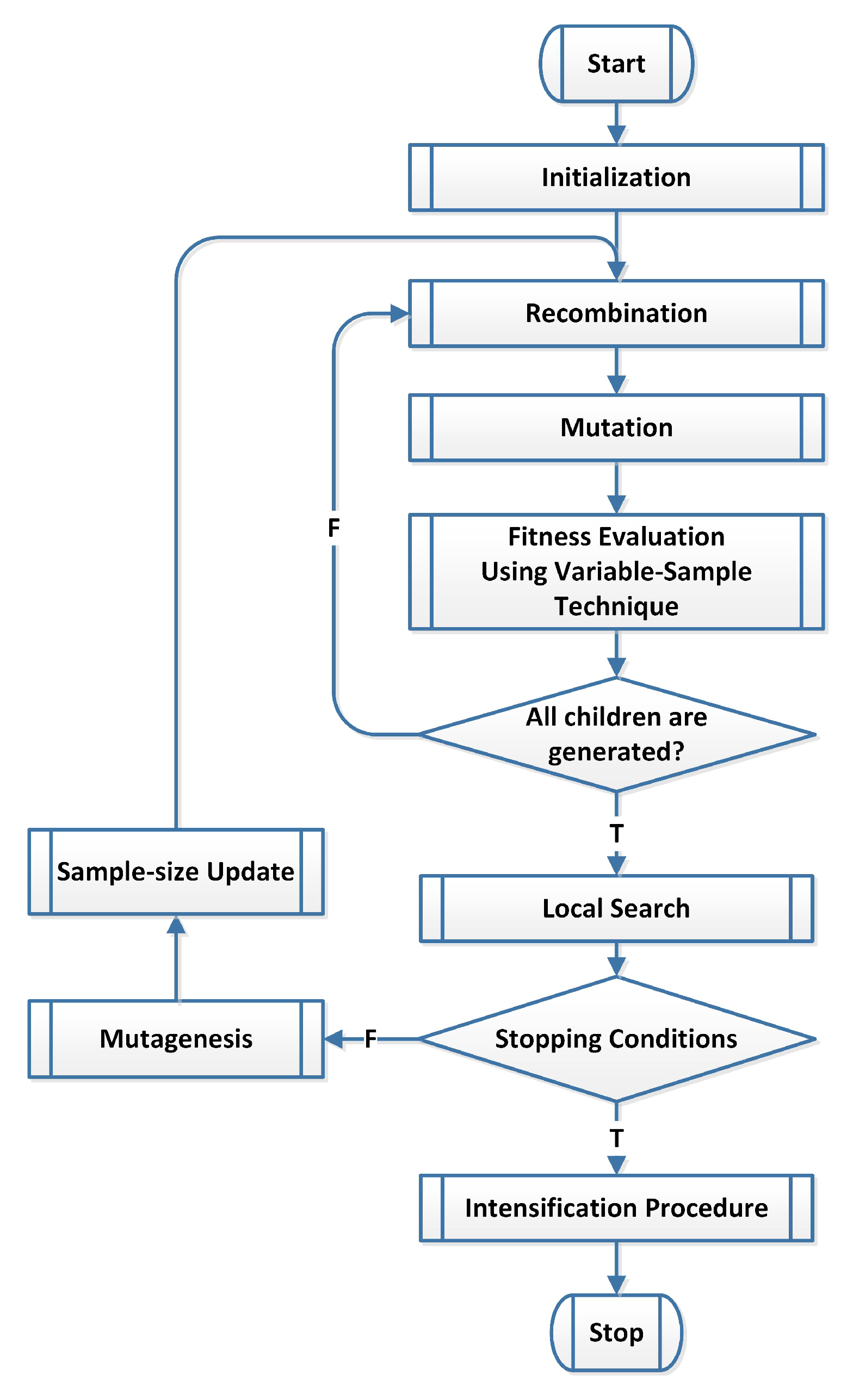
The DESSP method is a modified version of the DES method to handle the simulation-based global optimization problem. The modified version (DESSP) evaluates the fitness function values by employing the VS method (Algorithm 6). To illustrate how this can be done, Figure 4 and Figure 6 show the main structures of the DES and DESSP methods, respectively. One can note that the main added components in the DESSP method are the fitness function evaluation using variable sample technique and updating the size of the sample points. The first added component about function evaluations is performed as in Step 4 of Algorithm 6 with sample size N. The parameter is configured through the following procedure shown as Algorithm 7.
| Algorithm 7 |
|
In Algorithm 7, if is a value representing the status of getting a full GM, then sample size N is taken as a portion of . The lower and upper bounds of the sample size are a predefined value and , respectively.
6. Scatter Search for Simulation-Based Optimization
The DSS adapted to handle the same optimization problem using the following VS method.
6.1. Sampling and Fitness Evaluation
The VS technique is applied, as in Step 4 of Algorithm 6, to evaluate the objective (fitness) function, since it contains a random variable. The sample size parameter and its update are the main challenges with the fitness evaluation process. In the DSSSP method, the GM status can guide the configuration of the sample size parameter as described Sample Size Update Procedure (Algorithm 7).
6.2. DSSSP Algorithm
The DSS is modified to a new version called DSSSP, which tries to find the global optima in stochastic programming problems. Integrating the VS method into DSS is the main modification, Algorithm 6, to compute the fitness function values. The main steps in the DSSSP method are shown in Figure 7 and explained in Algorithm 8.
| Algorithm 8DSSSP Algorithm |
| 1: 2: repeat 3: Generate a solution x using the Diversification Generation Method. 4: if ( || is not close to any member in P) then, 5: . 6: end if 7: until the size of P is equal to . 8: Use variable sampling with size N to compute the fitness values for all members in P. 9: Apply Update with GM Procedure (Algorithm 4) to generate an initial RefSet. 10: while the stopping criteria are not met do 11: Use the Subset Generation Method to create solution subsets of size two. 12: Generate the offspring using the Combination Method. 13: Refine the offspring using the Improvement Method and add them to Set. 14: Use the Update with GM Procedure (Algorithm 4) to update the RefSet. 15: Update the variable sample size N using Sample Size Update Procedure (Algorithm 7). 16: end while 17: Refine the best solutions using a local search method. |
7. Numerical Experiments
The proposed methods have been implemented using MATLAB, and some benchmark test functions have been applied to evaluate their performance. In this section, the configuration and the main numerical results prove the efficiency of these methods are shown.
7.1. Test Functions
For the nonlinear programming problem, we have tested the proposed algorithms using two sets of well-known test functions Set A, and Set B. Table 1 contains Set A [41,42,43], while Set B is listed in Table 2. These two sets of functions have enough diverse characteristics to test different difficulties that arise in global optimization problems.
For the stochastic programming problem, seven test problems [44] are formulated from four documented test functions shown in Table 3, while their mathematical definitions are given in Appendix A [34].
7.2. Parameter Setting and Tuning
To have a complete description of the proposed algorithms, all setting parameters of the DES, DSS, DESSP, and DSSSP methods are discussed in this section. Table 4 and Table 5 summarize these parameters, their definitions, and best values. The values stated in the literature are used to set some parameters. A tuning process is carried out to obtain standard settings, while the proper values of the other parameters have been set by running some preliminary numerical experiments. These standard settings do not as much as possible, depend on the problem.
Different termination criteria are used in comparisons to stop the proposed methods. First, the automatic termination criterion based on the GM is discussed. We define ratio to be equal to the number of ones in GM divided by the total number of entities of GM. If is equal to 1 or closed to 1, then the method can learn that a wide exploration process has been achieved. Therefore, the algorithm can be stopped after satisfying the condition , where is equal to 1 or closed to 1. Figure 8 shows the results of applying the GM termination on the DESSP and DSSSP methods. In this figure, we allowed the algorithm to continue after reaching the termination point in order to notice any possible improvement after that. It is clear from the figure that there is almost no significant improvement after the GM termination point. The values of are set equal to and 1 for the DESSP and DSSSP methods, respectively. The difference in values is a result because the DESSP method uses the GM to update its iterate solution sets more than that in the DSSSP method. Therefore, the DSSSP method reaches a full GM faster than the DSSSP method. In comparisons, we terminated the proposed methods according to the same termination criterion used in the compared methods in order to get a fair comparison [45,46].
7.3. Numerical Results on Functions without Noise
This section contains the explanation of the experiments’ implementation that evaluates the proposed algorithms and show their results. Initially, two experiments are carried out to test the DSS algorithm. The first experiment measures the effect of applying Gene Matrix to the standard SS. The experimental results are reported after applying the SS algorithm with and without using GM on the Set A test functions stated in Table 1. On the other hand, the second one compares the performance of the DSS and the standard SS method as well as other metaheuristics methods.
The optimality gap of the above experiments is defined as:
where x and and are a heuristic solution, and the optimal solution, respectively. We consider x as a best solution if the average .
The results of the first experiment after updating RefSet with (DSS) and without using GM (standard SS) are reported in Table 6. These results are calculated after running each test function; ten independent runs with a maximum number of evaluating the objective function equals 20,000 for each run. The results, shown in Table 6, illustrate both the average gap (Av. GAP) and the success rates (Suc.) of all functions. The results, especially for the higher dimensional problems, reveal that the DSS algorithm has steadily better performance than the standard SS in terms of Av. GAP and the ability to obtain a global solution.
The average gap calculated using DSS algorithm, with the maximum number of function evaluation equals 50,000, is reported in Table 7 over the set of 40 functions listed as Set B in Table 2. The DSS algorithm closely reaches near to global solutions as proven from the results shown in Table 6 and Table 7.
A performance comparison is carried out in the second experiment between the DSS algorithm and standard Scatter Search (SS) algorithms [32] as well as the other two metaheuristics methods designed for the continuous optimization problems. These other two methods are the Genetic Algorithm (GA) for constrained problems (Genocop III) [47], and Directed Tabu Search (DTS) [43]. The results of the Av. GAP calculated over the 40 functions of Set B at several points during the search are shown in Table 8. The method [32] ignores the GAP for Problem 23; therefore, we also ignore the result of that problem and provide the results of 39 problems.
Our proposed DSS algorithm performs better than the SS as designed in [32], since the ; except problem 23 with . All the SS have , except problems 23, 26, 34, and 40, which have GAP values equal , , , and , respectively. Another comparison criteria is the number of solved problems. The DSS solves 33 problems after 50,000 function evaluations, however the SS [32] just solves 30 problems even with increasing the number of the functions evaluations from 20,000 up to 50,000.
The results in Table 8 show a substantial improvement of the values of Av. GAP applying DSS algorithm compared to the other methods at a large number of function evaluation. These results demonstrate the standing of the DSS method on the exploration process, which requests a high cost of function evaluations to guarantee good coverage to the search space. An additional performance measure is the number of optimal solutions found while applying each method.
Figure 9 illustrates the number of optimal solutions reached by each algorithm during the search process with a stopping condition of 50,000 objective function evaluations. The figure demonstrates a better performance of the DSS algorithm at a large number of function evaluations by solving 33 at 50,000 evaluations, while Genocop III, SS, and DTS successfully solve a total of 23, 30, and 32 problems, respectively.
7.4. Stochastic Programming Results
The main results of the DESSP and DSSSP methods are shown in Table 9, which includes the averages of the best and the average of the error gaps of the obtained solutions. These results obtained through 100 independent runs of the DESSP and DSSSP codes with a maximum number of function evaluations equal to 500,000 in each run. These results illustrate that the DSSSP could attain very close solutions for four test functions , , , and . The results for functions and are not so far from the optimal ones. However, due to the big size of function , the result of DESSP was not close to the optimal solution. Moreover, the DSSSP algorithm has revealed a best performance especially for high dimensional function . For four test functions and , the DSSSP can attain very close solutions, and the solutions for functions , , , and are near the optimal ones. The performance of the proposed methods is measured with more accurate metric called Normalized Distance [48], which is defined using three components as follows:
- Normalized Euclidean Distance ():where is the exact solution, is the approximate solution obtained by the proposed methods, and , are upper and lower bounds of the search space, respectively.
- Associate Normalized Distance ():where is the best minimum value of the objective function obtained by the proposed methods, and , are the global maximum and minimum values of the objective function, respectively, within the search space.
- Total Normalized Distance ():
Table 10 shows the values of these metrics for the results obtained by the DESSP and DSSSP methods.
Averages of processing time for running the DESSP and DSSSP codes are shown in Table 11. These averages are recorded in seconds after running the proposed codes on iMac machine with 3.2 GHz Quad-Core Intel Core i5 processor and 24 GB 1600 MHz DDR3 memory. The processing time of the DESSP code is better than that of the DSSSP code as shown in Table 11. However, the statistical test results in Table 12 do not favor either method against the other at the significance level 5%.
In order to clarify the performance difference between the proposed methods, we can use the Wilcoxon rank-sum test [49,50,51]. This test belongs to the class of non-parametric tests which are recommended in our experiments [52,53]. Table 12 summarizes the results of applying Wilcoxon test on the results obtained by the proposed methods, it displays the sum of rankings obtained in each comparison and the p-value associated. In this statistical test, we assume that is the difference between the performance scores of the two methods on i-th out of N results. Then, we rank the differences according to their absolute values. The ranks and are computed as follows:
The null hypothesis of equality of means is rejected if the is less than or equal to the value of the distribution of Wilcoxon for N degrees of freedom (Table B.12 in [51]).
Although the shown results indicate that the DESSP method is slightly better than the DSSSP method, the statistical test results in Table 12 show that there is no significant difference between the two methods at the significance level 5%.
The DESSP results have been compared against the results of the standard evolution strategies (ES) method and one of the best version of it which is called Covariance Matrix Adaptation Evolution Strategy (CMA-ES) [54]. The comparison results are shown in Table 13, which includes the averages of the best function values obtained by each method within 100 independent runs. From Table 13, the DESSP method has shown superior performance against the compared methods.
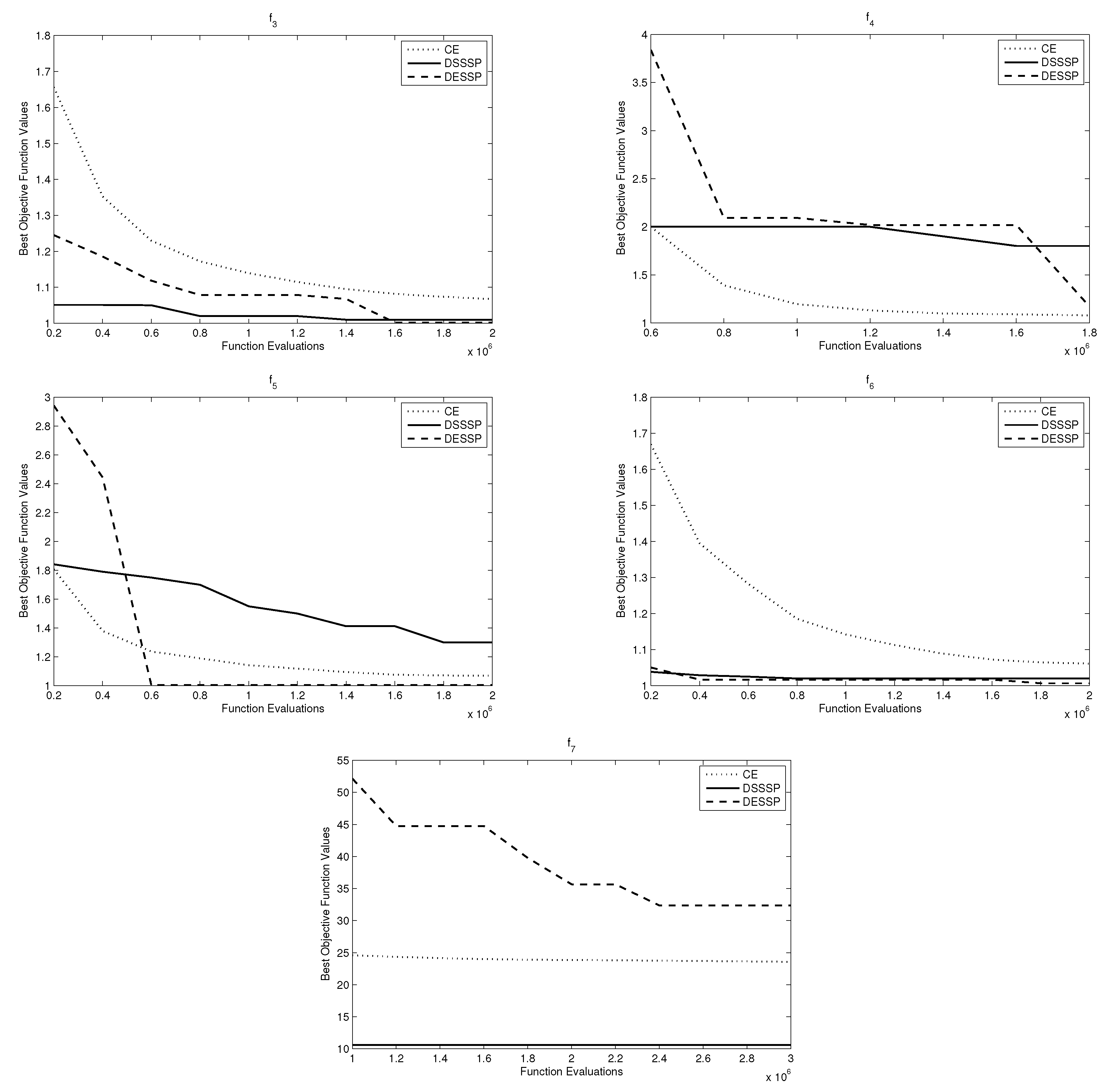
A comparison between the proposed methods and the Cross-Entropy method [44] is also carried out. Figure 10 shows the results, which promise potentials of the proposed methods in attaining better objective function values in some tested function. It is worthwhile to mention that the final intensification plays an important role in improving the obtained solutions, as shown in the method performance with function in Figure 10.
8. Conclusions
In this paper, novel algorithms are designed to search for a globally optimal solution or near-globally optimal solution of an objective function that having random noisy variables. The proposed methods combine a modified version of the scatter search and evolution strategies with a variable-sample method, which is a Monte-Carlo based to handle the random variables. Moreover, a memory element called gene matrix is invoked which could guide the search process to new diverse solutions and also help in terminating the algorithms. We have implemented these methods in MATLAB. The performance of these proposed methods is tested using several sets of benchmark test functions of nonlinear and stochastic programming problems. The obtained results proved that these novel methods have promising performance compared with some standard methods in the literature. As future work, many other metaheuristics can be adapted to deal with stochastic programming by invoking different sampling techniques in order to interface the problem of noise. In addition, the fuzzy and rough set theories can be modeled instead of sampling techniques to deal with the uncertainty of objective functions with noise.
Author Contributions
Conceptualization, A.-R.H. and A.A.A.; methodology, A.-R.H., A.A.A. and W.D.; software, A.A.A.; validation, A.-R.H. and A.A.A.; formal analysis, A.-R.H., A.A.A. and W.D.; investigation, A.-R.H. and A.A.A.; resources, A.-R.H., A.A.A. and W.D.; data Creation, A.A.A. and W.D.; writing—original draft preparation, A.-R.H. and A.A.A.; writing—review and editing, A.-R.H. and W.D.; visualization, A.-R.H., A.A.A. and W.D.; project administration, A.-R.H.; funding acquisition, A.-R.H.
Funding
This work was funded by the National Plan for Science, Technology and Innovation (MAARIFAH)—King Abdulaziz City for Science and Technology – the Kingdom of Saudi Arabia, award number (13-INF544-10).
Conflicts of Interest
The authors declare no conflict of interest.
Appendix A. Test Functions
Appendix A.1. Goldstein & Price Function
Search space:
Global minimum:
Appendix A.2. Rosenbrock Function
Search space:
Global minimum:
Appendix A.3. Griewank Function
Search space:
Global minimum:
Appendix A.4. Pinter Function
Search space:
Global minimum:
Appendix A.5. Modified Griewank Function
Search space:
Global minimum:
Appendix A.6. Griewank function with non-Gaussian Noise
The simulation noise is changed to the uniform distribution
Search space:
Global minimum:
Appendix A.7. Griewank Function (n = 50)
Search space:
Global minimum:
References
- Osorio, C.; Selvama, K.K. Simulation-based optimization: Achieving computational efficiency through the use of multiple simulators. Transp. Sci. 2017, 51, 395–411. [Google Scholar] [CrossRef]
- Campana, E.F.; Diez, M.; Iemma, U.; Liuzzi, G.; Lucidi, S. Derivative-free global ship design optimization using global/local hybridization of the DIRECT algorithm. Optim. Eng. 2016, 17, 127–156. [Google Scholar] [CrossRef]
- Pourhassan, M.R.; Raissi, S. An integrated simulation-based optimization technique for multi-objective dynamic facility layout problem. J. Ind. Inf. Integr. 2017, 8, 49–58. [Google Scholar] [CrossRef]
- Simpson, T.W.; Mauery, T.M.; Korte, J.J.; Mistree, F. Kriging models for global approximation in simulation-based multidisciplinary design optimization. AIAA J. 2001, 39, 2233–2241. [Google Scholar] [CrossRef]
- Schillings, C.; Schmidt, S.; Schulz, V. Computers & Fluids Efficient shape optimization for certain and uncertain aerodynamic design. Comput. Fluids 2011, 46, 78–87. [Google Scholar] [CrossRef]
- Hu, X.; Chen, X.; Parks, G.T.; Yao, W. Review of improved Monte Carlo methods in uncertainty-based design optimization for aerospace vehicles. Prog. Aerosp. Sci. 2016, 86, 20–27. [Google Scholar] [CrossRef]
- Hojjat, M.; Stavropoulou, E.; Bletzinger, K.U. The Vertex Morphing method for node-based shape optimization. Comput. Methods Appl. Mech. Eng. 2014, 268, 494–513. [Google Scholar] [CrossRef]
- Chong, L.; Osorio, C. A simulation-based optimization algorithm for dynamic large-scale urban transportation problems. Transp. Sci. 2017, 52, 637–656. [Google Scholar] [CrossRef]
- Mall, P.; Fidlin, A.; Krüger, A.; Groß, H. Simulation based optimization of torsional vibration dampers in automotive powertrains. Mech. Mach. Theory 2017, 115, 244–266. [Google Scholar] [CrossRef]
- Diez, M.; Volpi, S.; Serani, A.; Stern, F.; Campana, E.F. Simulation-Based Design Optimization by Sequential Multi-criterion Adaptive Sampling and Dynamic Radial Basis Functions. In Advances in Evolutionary and Deterministic Methods for Design, Optimization and Control in Engineering and Sciences; Springer International Publishing AG: Cham, Switzerland, 2019; Volume 48, pp. 213–228. [Google Scholar] [CrossRef]
- Gosavi, A. Simulation-Based Optimization: Parametric Optimization Techniques and Reinforcement Learning; Springer: New York, NY, USA, 2015. [Google Scholar]
- Birge, J.R.; Louveaux, F. Introduction to Stochastic Programming; Springer Science & Business Media: New York, NY, USA, 2011. [Google Scholar]
- Andradóttir, S. Simulation optimization. In Handbook of Simulation: Principles, Methodology, Advances, Applications, and Practice; John Wiley & Sons: New York, NY, USA, 1998; pp. 307–333. [Google Scholar]
- BoussaïD, I.; Lepagnot, J.; Siarry, P. A survey on optimization metaheuristics. Inf. Sci. 2013, 237, 82–117. [Google Scholar] [CrossRef]
- Glover, F.; Laguna, M.; Marti, R. Scatter search and path relinking: Advances and applications. In Handbook of Metaheuristics; Springer: Boston, MA, USA, 2003; pp. 1–35. [Google Scholar]
- Ribeiro, C.; Hansen, P. Essays and Surveys in Metaheuristics; Springer Science & Business Media: New York, NY, USA, 2002. [Google Scholar]
- Siarry, P. Metaheuristics; Springer International Publishing: Cham, Switzerland, 2016. [Google Scholar]
- Kvasov, D.E.; Mukhametzhanov, M.S. Metaheuristic vs. deterministic global optimization algorithms: The univariate case. Appl. Math. Comput. 2017, 318, 245–259. [Google Scholar] [CrossRef]
- Georgieva, A.; Jordanov, I. Hybrid metaheuristics for global optimization: A comparative study. In Hybrid Artificial Intelligence Systems; Lecture Notes in Computer Science (Including Subseries Lecture Notes in Artificial Intelligence and Lecture Notes in Bioinformatics); Springer: Berlin/Heidelberg, Germany, 2008; Volume 5271, pp. 298–305. [Google Scholar] [CrossRef]
- Liberti, L.; Kucherenko, S. Comparison of deterministic and stochastic approaches to global optimization. Int. Trans. Oper. Res. 2005, 12, 263–285. [Google Scholar] [CrossRef]
- Törn, A.; Ali, M.M.; Viitanen, S. Stochastic Global Optimization: Problem Classes and Solution Techniques. J. Glob. Optim. 1999, 14, 437–447. [Google Scholar] [CrossRef]
- Serani, A.; Diez, M. Are Random Coefficients Needed in Particle Swarm Optimization for Simulation-Based Ship Design? In Proceedings of the VII International Conference on Computational Methods in Marine Engineering, Nantes, France, 15–17 May 2017.
- Battiti, R.; Brunato, M.; Mascia, F. Reactive Search and Intelligent Optimization; Springer Science & Business Media: New York, NY, USA, 2008; Volume 45. [Google Scholar]
- Jordanov, I.; Georgieva, A. Neural network learning With global heuristic search. IEEE Trans. Neural Netw. 2007, 18, 937–942. [Google Scholar] [CrossRef]
- Lu, Y.; Zhou, Y.; Wu, X. A Hybrid Lightning Search Algorithm-Simplex Method for Global Optimization. Discrete Dyn. Nat. Soc. 2017, 2017. [Google Scholar] [CrossRef]
- Blum, C.; Roli, A. Hybrid Metaheuristics: An Introduction. In Hybrid Metaheuristics: An Emerging Approach to Optimization; Springer: Berlin/Heidelberg, Germany, 2008; pp. 1–30. [Google Scholar] [CrossRef]
- D’Andreagiovanni, F.; Krolikowski, J.; Pulaj, J. A fast hybrid primal heuristic for multiband robust capacitated network design with multiple time periods. Appl. Soft Comput. J. 2015, 26, 497–507. [Google Scholar] [CrossRef]
- Renders, J.M.; Flasse, S.P. Hybrid methods using genetic algorithms for global optimization. IEEE Trans. Syst. Man Cybern. Part B Cybern. 1996, 26, 243–258. [Google Scholar] [CrossRef]
- Homem-De-Mello, T. Variable-sample methods for stochastic optimization. ACM Trans. Model. Comput. Simul. (TOMACS) 2003, 13, 108–133. [Google Scholar] [CrossRef]
- Hedar, A.; Fukushima, M. Evolution strategies learned with automatic termination criteria. In Proceedings of the SCIS-ISIS, Tokyo, Japan, 20–24 September 2006; pp. 1126–1134. [Google Scholar]
- Sulaiman, M.; Salhi, A. A seed-based plant propagation algorithm: The feeding station model. Sci. World J. 2015, 2015. [Google Scholar] [CrossRef]
- Laguna, M.; Martí, R. Experimental testing of advanced scatter search designs for global optimization of multimodal functions. J. Glob. Optim. 2005, 33, 235–255. [Google Scholar] [CrossRef]
- Duarte, A.; Martí, R.; Glover, F.; Gortazar, F. Hybrid scatter tabu search for unconstrained global optimization. Ann. Oper. Res. 2011, 183, 95–123. [Google Scholar] [CrossRef]
- Hedar, A.; Ong, B.T.; Fukushima, M. Genetic Algorithms with Automatic Accelerated Termination; Tech. Rep; Department of Applied Mathematics and Physics, Kyoto University: Kyoto, Japan, 2007; Volume 2. [Google Scholar]
- Beyer, H.; Schwefel, H. Evolution strategies—A comprehensive introduction. Natural Comput. 2002, 1, 3–52. [Google Scholar] [CrossRef]
- Eiben, A.E.; Smith, J.E. Introduction to Evolutionary Computing; Springer-Verlag: Berlin/Heidelberg, Germany, 2003. [Google Scholar]
- Herrera, F.; Lozano, M.; Verdegay, J.L. Tackling real-coded genetic algorithms: Operators and tools for behavioural analysis. Artif. Intell. Rev. 1998, 12, 265–319. [Google Scholar] [CrossRef]
- Holstein, D.; Moscato, P. Memetic algorithms using guided local search: A case study. In New Ideas in Optimization; McGraw-Hill Ltd.: Maidenhead, UK, 1999; pp. 235–244. [Google Scholar]
- Ong, Y.S.; Keane, A.J. Meta-Lamarckian learning in memetic algorithms. Evol. Comp. IEEE Trans. 2004, 8, 99–110. [Google Scholar] [CrossRef]
- Ong, Y.; Lim, M.; Zhu, N.; Wong, K. Classification of adaptive memetic algorithms: a comparative study. Syst. Man Cybern. Part B Cybern. IEEE Trans. 2006, 36, 141–152. [Google Scholar]
- Hedar, A.; Fukushima, M. Minimizing multimodal functions by simplex coding genetic algorithm. Optim. Methods Softw. 2003, 18, 265–282. [Google Scholar] [CrossRef]
- Floudas, C.; Pardalos, P.; Adjiman, C.; Esposito, W.; Gumus, Z.; Harding, S.; Klepeis, J.; Meyer, C.; Schweiger, C. Handbook of Test Problems in Local and Global Optimization; Springer Science & Business Media: New York, NY, USA, 1999. [Google Scholar]
- Hedar, A.; Fukushima, M. Tabu search directed by direct search methods for nonlinear global optimization. Eur. J. Oper. Res. 2006, 170, 329–349. [Google Scholar] [CrossRef]
- He, D.; Lee, L.H.; Chen, C.H.; Fu, M.C.; Wasserkrug, S. Simulation optimization using the cross-entropy method with optimal computing budget allocation. ACM Trans. Model. Comput. Simul. (TOMACS) 2010, 20, 4. [Google Scholar] [CrossRef]
- Črepinšek, M.; Liu, S.H.; Mernik, L. A note on teaching–learning-based optimization algorithm. Inf. Sci. 2012, 212, 79–93. [Google Scholar] [CrossRef]
- Črepinšek, M.; Liu, S.H.; Mernik, M. Replication and comparison of computational experiments in applied evolutionary computing: Common pitfalls and guidelines to avoid them. Appl. Soft Comput. 2014, 19, 161–170. [Google Scholar] [CrossRef]
- Michalewicz, Z.; Nazhiyath, G. Genocop III: A co-evolutionary algorithm for numerical optimization problems with nonlinear constraints. In Proceedings of the 1995 IEEE International Conference on Evolutionary Computation, Perth, WA, Australia, 29 November–1 December 1995; Volume 2, pp. 647–651. [Google Scholar]
- Serani, A.; Leotardi, C.; Iemma, U.; Campana, E.F.; Fasano, G.; Diez, M. Parameter selection in synchronous and asynchronous deterministic particle swarm optimization for ship hydrodynamics problems. Appl. Soft Comput. 2016, 49, 313–334. [Google Scholar] [CrossRef] [Green Version]
- García, S.; Fernández, A.; Luengo, J.; Herrera, F. A study of statistical techniques and performance measures for genetics-based machine learning: Accuracy and interpretability. Soft Comput. 2009, 13, 959–977. [Google Scholar] [CrossRef]
- Sheskin, D.J. Handbook of Parametric and Nonparametric Statistical Procedures; CRC Press: Boca Raton, FL, USA; London, UK; New York, NY, USA; Washington, DC, USA, 2003. [Google Scholar]
- Zar, J.H. Biostatistical Analysis, 5th ed.; Pearson New International Edition: Essex, UK, 2013. [Google Scholar]
- Derrac, J.; García, S.; Molina, D.; Herrera, F. A practical tutorial on the use of nonparametric statistical tests as a methodology for comparing evolutionary and swarm intelligence algorithms. Swarm Evol. Comput. 2011, 1, 3–18. [Google Scholar] [CrossRef]
- García, S.; Molina, D.; Lozano, M.; Herrera, F. A study on the use of non-parametric tests for analyzing the evolutionary algorithms’ behaviour: A case study on the CEC’2005 special session on real parameter optimization. J. Heuristics 2009, 15, 617–644. [Google Scholar] [CrossRef]
- Hansen, N. The CMA evolution strategy: A comparing review. In Towards a New Evolutionary Computation; Springer-Verlag: Berlin/Heidelberg, Germany, 2006; pp. 75–102. [Google Scholar]
Figure 1.
An example of GM in a two-dimension search space.

Figure 2.
An example of the recombination operation.

Figure 3.
The role of recombination operation and GM.

Figure 4.
The structure of the DES method.

Figure 5.
The structure of the DSS method.

Figure 6.
The structure of the DESSP method.

Figure 7.
The structure of the DSSSP method.

Figure 8.
Automatic termination based on the GM.

Figure 9.
Number of solved problems.

Figure 10.
Comparison using test functions –.


Table 1.
Test functions for global optimization: Set A.
| No. | f | Function Name | n | No. | f | Function Name | n |
|---|---|---|---|---|---|---|---|
| 1 | Branin RCOS | 2 | 8 | Rastrigin | 10 | ||
| 2 | GoldsteinPrice | 2 | 9 | Rosenbrock | 10 | ||
| 3 | Rosenbrock | 2 | 10 | Rastrigin | 20 | ||
| 4 | Hartmann | 3 | 11 | Rosenbrock | 20 | ||
| 5 | Shekel | 4 | 12 | Powell | 24 | ||
| 6 | Perm | 4 | 13 | DixonPrice | 25 | ||
| 7 | Trid | 6 | 14 | Ackley | 30 |
Table 2.
Test functions for global optimization: Set B.
| No. | Function Name | f | n | No. | Function Name | f | n |
|---|---|---|---|---|---|---|---|
| 1 | Branin RCOS | 2 | 2 | Bohachevsky | 2 | ||
| 3 | Easom | 2 | 4 | Goldstein Price | 2 | ||
| 5 | Shubert | 2 | 6 | Beale | 2 | ||
| 7 | Booth | 2 | 8 | Matyas | 2 | ||
| 9 | Hump | 2 | 10 | Schwefel | 2 | ||
| 11 | Rosenbrock | 2 | 12 | Zakharov | 2 | ||
| 13 | De Joung | 3 | 14 | Hartmann | 3 | ||
| 15 | Colville | 4 | 16 | Shekel | 4 | ||
| 17 | Shekel | 4 | 18 | Shekel | 4 | ||
| 19 | Perm | 4 | 20 | Perm | 4 | ||
| 21 | Power Sum | 4 | 22 | Hartmann | 6 | ||
| 23 | Schwefel | 6 | 24 | Trid | 6 | ||
| 25 | Trid | 10 | 26 | Rastrigin | 10 | ||
| 27 | Griewank | 10 | 28 | Sum Squares | 10 | ||
| 29 | Rosenbrock | 10 | 30 | Zakharov | 10 | ||
| 31 | Rastrigin | 20 | 32 | Griewank | 20 | ||
| 33 | Sum Squares | 20 | 34 | Rosenbrock | 20 | ||
| 35 | Zakharov | 20 | 36 | Powell | 24 | ||
| 37 | DixonPrice | 25 | 38 | Levy | 30 | ||
| 39 | Sphere | 30 | 40 | Ackley | 30 |
Table 3.
Stochastic programming test functions.
| Function | Name | n | Stochastic Variable Distribution |
|---|---|---|---|
| Goldstein & Price | 2 | ||
| Rosenbrock | 5 | ||
| Griewank | 2 | ||
| Pinter | 5 | ||
| Modified Griewank | 2 | ||
| Griewank | 2 | ||
| Griewank | 50 |
Table 4.
DES and DESSP parameters.
| Parameter | Definition | Best Value |
|---|---|---|
| The population size | 50 | |
| The offspring size | ||
| No. of mated parents | ||
| The recombination probability | ||
| The initial value for the sample size | 100 | |
| The maximum value for the sample size | 5000 | |
| No. of best solutions used in in the intensification step | 1 | |
| No. of worst solutions updated by the mutagenesis process | n | |
| m | No. of partitions in GM | 50 |
Table 5.
DSS and DSSSP parameters.
| Parameter | Definition | Best Value |
|---|---|---|
| Psize | The initial population size | 100 |
| b | The size of the RefSet | 10 |
| No. of elite solutions in RefSet | 6 | |
| No. of diverse solutions in RefSet | 4 | |
| The initial value for the sample size | 100 | |
| The maximum value for the sample size | 5000 | |
| No. of best solutions used in in the intensification step | 1 | |
| No. of worst solutions updated by the mutagenesis process | 3 | |
| m | No. of partitions in GM | 50 |
Table 6.
DSS and SS results on Set A.
| f | SS | DSS | ||
|---|---|---|---|---|
| Av. GAP | Suc. | Av. GAP | Suc. | |
| 3.58 | 100 | 3.581 | 100 | |
| 4.69 | 100 | 5.35 | 100 | |
| 1.1 | 100 | 2.56 | 100 | |
| 2.1 | 100 | 2.15 | 100 | |
| 2.9 | 100 | 3.22 | 100 | |
| 0.6 | 13 | 0.55 | 27 | |
| 2.39 | 80 | 2.703 | 77 | |
| 4.66 | 100 | 1.92 | 100 | |
| 18.59 | 0 | 15.01 | 0 | |
| 3.558 | 0 | 5.01 | 0 | |
| 45.84 | 0 | 29.77 | 0 | |
| 47.1 | 0 | 16.2 | 0 | |
| 3.51 | 0 | 1.4 | 0 | |
| 10.39 | 0 | 8.28 | 0 | |
Table 7.
DSS results on Set B.
| No. | f | Av. GAB | No. | f | Av. GAB |
|---|---|---|---|---|---|
| 1 | 3.5773 | 2 | 0 | ||
| 3 | 0 | 4 | 7.7538 | ||
| 5 | 8.83102 | 6 | 0 | ||
| 7 | 0 | 8 | 1.73546 | ||
| 9 | 4.65101 | 10 | 2.54551 | ||
| 11 | 0 | 12 | 2.88141 | ||
| 13 | 9.77667 | 14 | 2.14782 | ||
| 15 | 2.05 | 16 | 3.41193 | ||
| 17 | 5.66819 | 18 | 9.81669 | ||
| 19 | 3.83 | 20 | 5.52274 | ||
| 21 | 6.09758 | 22 | 2.05919 | ||
| 23 | 78.99516181 | 24 | 7.58971 | ||
| 25 | 8.06413 | 26 | 1.91653 | ||
| 27 | 0.142472164 | 28 | 3.75918 | ||
| 29 | 0.707283407 | 30 | 1.9217 | ||
| 31 | 7.98934 | 32 | 0.052065617 | ||
| 33 | 5.41513 | 34 | 0.739935703 | ||
| 35 | 0.19800033 | 36 | 8.33102 | ||
| 37 | 0.943358525 | 38 | 1.29657 | ||
| 39 | 1.26068 | 40 | 1.08842 |
Table 8.
The comparison results of DSS and other metaheuristics.
| Evaluations | Genocop III | SS | DTS | DSS |
|---|---|---|---|---|
| 500 | 611.30 | 26.34 | 43.06 | 112.08 |
| 1000 | 379.03 | 14.66 | 24.26 | 56.24 |
| 5000 | 335.81 | 4.96 | 4.22 | 34.88 |
| 10,000 | 328.66 | 3.60 | 1.80 | 5.36 |
| 20,000 | 324.72 | 3.52 | 1.70 | 0.9031 |
| 50,000 | 321.20 | 3.46 | 1.29 | 0.0714 |
Table 9.
Error gap results obtained by the DESSP and DSSSP methods.
| f | DESSP | DSSSP | ||
|---|---|---|---|---|
| Best | Average | Best | Average | |
| 0.0005 | 0.2326 | 0.0146 | 0.2939 | |
| 0.8046 | 3.5496 | 0.4080 | 6.5550 | |
| 0.0010 | 0.3313 | 0.5900 | 1.0400 | |
| 0.1442 | 3.7538 | 2.7487 | 6.7145 | |
| 0.0004 | 0.3871 | 0.2819 | 1.9135 | |
| 0.00001 | 0.0213 | 0.0003 | 0.0921 | |
| 27.8824 | 39.5636 | 8.4088 | 12.3794 | |
Table 10.
Averages of normalized Euclidean distances obtained by the DESSP and DSSSP methods.
| DESSP | DSSSP | |||||
|---|---|---|---|---|---|---|
| 8.1364 | 2.2982 | 5.7533 | 4.1030 | 2.9045 | 2.9013 | |
| 1.2902 | 7.3332 | 9.1231 | 4.2088 | 1.3542 | 2.9761 | |
| 1.3467 | 5.0255 | 3.8547 | 7.9792 | 1.5776 | 1.2763 | |
| 1.0589 | 9.7511 | 7.4884 | 2.5053 | 2.0036 | 17.7155 | |
| 1.0925 | 5.0989 | 3.8599 | 6.6194 | 2.5204 | 1.8554 | |
| 7.6039 | 3.2361 | 6.6166 | 2.2119 | 1.3976 | 2.0627 | |
| 1.6132 | 1.6105 | 1.6134 | 2.7005 | 5.0392 | 1.9430 | |
Table 11.
Averages of processing time (in seconds) for running the DESSP and DSSSP codes.
| f | |||||||
|---|---|---|---|---|---|---|---|
| DESSP | 162 | 20 | 119 | 177 | 25 | 10 | 476 |
| DSSSP | 414 | 103 | 317 | 307 | 114 | 35 | 683 |
Table 12.
Wilcoxon rank-sum test of DESSP and DSSSP results.
| Comparison Criteria | p-Value | Best Method | ||
|---|---|---|---|---|
| Best Solutions | 11 | 17 | 0.3829 | – |
| Average Solutions | 7 | 21 | 0.6200 | – |
| 8 | 28 | 0.0973 | – | |
| 6 | 22 | 0.7104 | – | |
| 0 | 28 | 0.3176 | – | |
| Processing Time | 0 | 28 | 0.2593 | – |
Table 13.
The averages of the best function values obtained by ES, CMA-ES, and DESSP.
| Method | ||||
|---|---|---|---|---|
| ES | 47.7325 | 3.265 | 970.7125 | |
| CMA-ES | 13.2173 | 12.7998 | 2.4712 | 23.6619 |
| DESSP | 3.0005 | 1.8046 | 1.0010 | 1.1442 |
© 2019 by the authors. Licensee MDPI, Basel, Switzerland. This article is an open access article distributed under the terms and conditions of the Creative Commons Attribution (CC BY) license (http://creativecommons.org/licenses/by/4.0/).
Share and Cite
MDPI and ACS Style
Hedar, A.-R.; Allam, A.A.; Deabes, W. Memory-Based Evolutionary Algorithms for Nonlinear and Stochastic Programming Problems. Mathematics 2019, 7, 1126. https://0-doi-org.brum.beds.ac.uk/10.3390/math7111126
AMA Style
Hedar A-R, Allam AA, Deabes W. Memory-Based Evolutionary Algorithms for Nonlinear and Stochastic Programming Problems. Mathematics. 2019; 7(11):1126. https://0-doi-org.brum.beds.ac.uk/10.3390/math7111126
Chicago/Turabian StyleHedar, Abdel-Rahman, Amira A. Allam, and Wael Deabes. 2019. "Memory-Based Evolutionary Algorithms for Nonlinear and Stochastic Programming Problems" Mathematics 7, no. 11: 1126. https://0-doi-org.brum.beds.ac.uk/10.3390/math7111126
Note that from the first issue of 2016, this journal uses article numbers instead of page numbers. See further details here.