Long Term Memory Assistance for Evolutionary Algorithms

Abstract

Short term memory that records the current population has been an inherent component of Evolutionary Algorithms (EAs). As hardware technologies advance currently, inexpensive memory with massive capacities could become a performance boost to EAs. This paper introduces a Long Term Memory Assistance (LTMA) that records the entire search history of an evolutionary process. With LTMA, individuals already visited (i.e., duplicate solutions) do not need to be re-evaluated, and thus, resources originally designated to fitness evaluations could be reallocated to continue search space exploration or exploitation. Three sets of experiments were conducted to prove the superiority of LTMA. In the first experiment, it was shown that LTMA recorded at least $50\%$ more duplicate individuals than a short term memory. In the second experiment, ABC and jDElscop were applied to the CEC-2015 benchmark functions. By avoiding fitness re-evaluation, LTMA improved execution time of the most time consuming problems $F03$ and $F05$ between 7% and 28% and 7% and 16%, respectively. In the third experiment, a hard real-world problem for determining soil models’ parameters, LTMA improved execution time between 26% and 69%. Finally, LTMA was implemented under a generalized and extendable open source system, called EARS. Any EA researcher could apply LTMA to a variety of optimization problems and evolutionary algorithms, either existing or new ones, in a uniform way.

1. Introduction

Evolutionary Algorithms (EAs) [1] are stochastic algorithms that originated by utilizing nature-inspired behaviors to search for the global optimum/optima. Over the past few decades, EA research communities concentrated their efforts on expanding EA areas by mimicking a variety of nature-inspired behaviors (e.g., ABC [2], ACO [3], Grasshopper Optimization Algorithm (GOA) [4], Gray Wolf Optimizer (GWO) [5], PSO [6], and Teaching-Learning Based Optimization (TLBO) [7]), although, in many cases, searching for inspiration from nature has gone too far [8]. EA researchers also dedicated themselves to how EA’s parameters may influence the evolutionary processes (e.g., parameter-less [9], parameter tuning [10,11], and parameter control [12,13]). Both research mainstreams (i.e., EA behaviors and EA parameters) consider EAs as balancing an evolutionary process between exploration and exploitation [14], either by controlling EA operations, or EA parameters, or both.

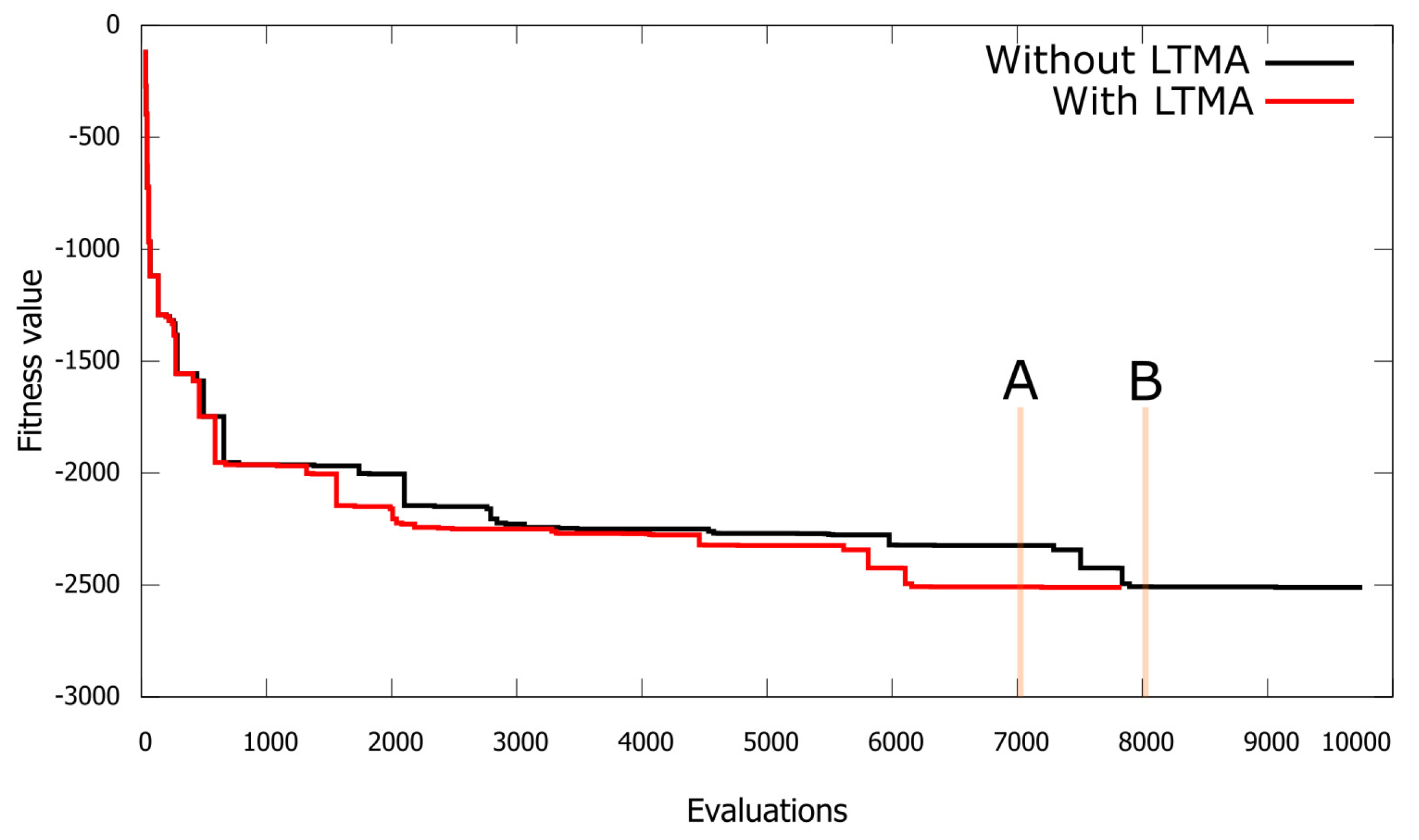
Although duplicate individuals (revisited solutions) have been recognized as unproductive from the beginning of EAs, not enough research has been done to evaluate how costly it is to identify duplicates and how much benefit can be gained if duplicates can be identified and replaced with new solutions. For example, Koza wrote in [15]: “Duplicate individuals in the initial random generation are unproductive deadwood; they waste computational resources and reduce the genetic diversity of the population” undesirably. However, duplicate individuals in Genetic Programming (GP) [15] have been identified only in initial random generation. This is because duplicate random individuals are especially likely to be generated when the trees are small, and discovering duplicates in the later phases when the trees are large would be a costly process, not to mention the cost of keeping track of all solutions (trees in the case of GP) over the entire evolutionary process (over all generations). In Teaching-Learning Based Optimization (TLBO) [7], a duplicate elimination phase has been introduced to replace duplicates generated in one generation with random solutions, but duplicates were not checked with previous solutions found in earlier generations. Even more importantly, in TLBO, fitness evaluations were re-computed on duplicates and only later replaced with random solutions consuming more fitness evaluations [16,17]. The immediate question that arises is: How much can we profit if fitness evaluations are not re-computed on duplicates, and how costly is it to discover duplicates over the whole evolutionary process? However, the question is if this problem is real. Do EAs indeed generate many duplicates? We have often used the Artificial Bee Colony (ABC) algorithm in the past [18,19] and discovered that ABC exploitation performed in employed and onlooker bee phases actually generates many duplicates. Figure 1 shows one such example of using ABC where a convergence graph with duplicates (without Long Term Memory Assistance (LTMA)) is compared with a convergence graph with no duplicates (with LTMA), where duplicates are rather replaced with new solutions. For a fair comparison, a single run was used for both scenarios (red and black lines). LTMA was simulated based on a full run, by removing duplicate solutions that, in the case of using LTMA, would not be generated. As a result, the algorithm with LTMA converged earlier (the flat parts of the line are shorter, where duplicates were generated). Even in this simple example (Figure 1), it is clear that gains can be substantial (e.g., Solution A with Long Term Memory Assistance (LTMA) in Figure 1 can be found at least 1000 evaluations earlier than the same Solution B without LTMA). Especially in real-world problems where fitness evaluations are costly, we can expect large gains on CPU time by not re-computing fitness evaluations of duplicates or even better solutions when duplicates are rather replaced with new solutions enhancing the exploration and exploitation of the search space. However, how much we can gain from discovering duplicates and replacing them with new solutions has not been tested before. Hence, we decided to explore this topic more deeply on problems where solutions are represented as a vector of real numbers. Using graphs and trees (e.g., as in GP) as representations of solutions is out of the scope of this study.

In this paper, we call solutions (population) in the current generation short term memory and all solutions tested so far from the initial population long term memory. When using only the short term memory, we lose information on which solutions have already been visited (generated) in the previous generations, and it is quite possible that some solutions were re-visited. Re-evaluation of duplicate individuals is an unnecessary step and can be eliminated if we have long term memory. In this work, Long Term Memory Assistance (LTMA) is introduced, which can increase efficiency in terms of EA convergence.

The main contributions of this study are:

• estimation of the cost (memory and CPU time usage) for duplicate identification when solutions are represented as a vector of real numbers,
• estimation of how many fitness evaluations can be saved by not re-evaluating existing solutions for a few selected EAs and problems,
• demonstrating how we can “attach” long term memory in a uniform way to existing EAs and provide a general solution for this topic.

This paper is organized as follows. In Section 2, related work on how the past partial or complete search history has been recorded and utilized is reviewed briefly. The motivation of the research is proposed in Section 3. In Section 4, the proposed LTMA and its implementation are described briefly. In Section 5, duplicates’ generation is analyzed, as well as their effects on benchmark and real-world problems. Finally, the paper concludes in Section 6.

2. Related Work

For EAs, the short term memory concept has been an essential component realized through selection processes. For example, genetic algorithms [20] utilize a selection process to choose individuals for the next generation randomly, based on different strategies (e.g., tournament selection and fitness proportional selection). Although most selection processes use fitness values to guide selection, due to random selection, fitter individuals are not necessarily guaranteed to propagate to the next generation. Later, Evolution Strategies (ESs) [20] introduced a deterministic approach to select individuals based on the fitness ranking of individuals. Survival is guaranteed for a certain number of current best individuals. For example, (1+1)-ESs select the best between the parent and its mutated offspring for the next generation. Elitism represents an important milestone of introducing the long term memory concept to single-objective evolutionary algorithms [20,21], such that the current best individual(s) can survive throughout the evolutionary process. The elitism concept was later adapted as an external archive in most multi-objective evolutionary algorithms. All the non-dominated solutions found during the evolutionary process are retained in an external archive, so that they can be used to compare with current solutions. Some notable examples are SPEA2 [22], PAES [23], and EAG-MOEA/D [24]. Note that, although external archives are a commonly used approach in multi-objective evolutionary algorithms, NSGA-II [25] and its successor NSGA-III [26] still adopt elitism to retain the best individuals from both parents and offspring. External archives are also applied to some single-objective evolutionary algorithms. For example, JADE [27] introduced an optional external archive that stores a set of recently explored inferior solutions to guide the evolutionary process and improve diversity. Tanabe and Fukunaga [28] extended JADE, but recorded the history of parameters instead of recently explored solutions. Another EA sub-area that utilizes memory mechanisms is changing optimization problems or dynamic/uncertain environments [29,30,31,32]. Since this paper does not discuss changing optimization problems, readers may refer to those related works if interested.

Note that, although elitism or external archives introduced long term memory concepts to single-objective and multi-objective evolutionary algorithms, only partial solutions are recorded from the entire evolutionary process. During the past decade, several EA researchers have introduced new data structures to store the information obtained during the entire evolutionary process. For example, Chow and Yeun introduced non-revising GA [33] and the history driven evolutionary algorithm [34]. Both algorithms utilize the Binary Space Partition (BSP) tree to partition the search space and memorize the search history to avoid revisiting same solutions. They also introduced the continuous Non-revisiting Genetic Algorithm (cNrGA) for continuous variables and, later, introduced pruning mechanisms to maintain constant memory usage [35]. Leung et al. [36] extended the work to utilize past history to compute an approximate fitness landscape to control the evolutionary processes. Zhang and Wu [37] applied a BSP tree to the ABC algorithm to record and utilize the entire search history to improve the quality of regenerated solutions from the scout bee phase. Zabihi and Nasiri also applied a BSP tree to ABC algorithms for data clustering [38]. Nasiri et al. [39] used a BSP tree to approximate the landscape information of dynamic and uncertain optimization problems. In addition to a BSP tree, Črepinšek et al. [40] introduced an ancestry tree data structure to record the evolution history of a population and invented exploration and exploitation metrics based on the tree structure.

From the above discussions and references, long term memory has been proven as a useful mechanism for many EAs. Yet, due to memory constraints and the focus of introducing or improving EAs, to our best knowledge, there have not been many related works on recording and memorizing the entire search history of an evolutionary process for long term memory, where the cost of identifying re-visited solutions and the profit of not re-computing fitness evaluations have been investigated. Additionally, the aforementioned related work applied the entire search history for specific algorithms. LTMA, conversely, provides a general and extendable solution by decoupling long term memory from algorithms and problems.

Please note that Long Short-Term Memory (LSTM) [41] has been introduced in the deep learning research field (e.g., [42,43,44,45]). Unlike LTMA, LSTM introduces cells and gates to form a “highway” to retain gradient information in a long sequence of a recurrent neural network. In [46], a genetic algorithm was integrated with an LSTM network to optimize time window size and architectural factors, to better predict the Korea Composite Stock Price Index.

3. Memory

3.1. How Much Memory Do We Need?

To calculate how much memory we need for completing long term memory recall, we need to know some data about the EA used, the problem being solved, and its stopping criteria. In our work, the following assumptions were made:

• Only memory needed to store all individuals (populations over whole generations) is computed, although different EAs need extra memory for additional computations. This algorithm specific memory usage is not taken into account in our work.
• Only single-objective continuous optimization problems have been studied, where a point in a search space (genotype) is represented as a vector x of length n, $x\in {\Re }^n$, and fitness (phenotype) $y=f\left(x\right)\in \Re$. To represent a real value ℜ, often eight bytes of memory are used (e.g., Java). Therefore, $(n+1)*8$ bytes are needed for one member of a population and its fitness value. A different memory consumption is needed in the case of discrete optimization, where the representation of a population member is problem dependent. In the case of multi-objective optimization, a solution $y\in {\Re }^k$ (k^th objectives) and more memory are needed to store a fitness value.
• The stopping criteria determine how many solutions are going to be generated. The fixed-cost (vertical) and the fixed-target (horizontal) approaches were identified in [47]. In the fixed-cost approach, solutions are generated until we reach a pre-defined number of iterations, or pre-defined number of fitness evaluations ($MFES$), or pre-defined CPU time. In the fixed-target approach, solutions are generated until a (sub-)optimal solution is found. Some hybrid stopping criteria, blending vertical and horizontal approaches, have also been employed in EAs. Among the aforementioned approaches, it is often unknown how many solutions will be generated (e.g., based on CPU time or based on the maximum number of iterations when some extra local search is also included). Hence, in this study, $MFES$ is used as a stopping condition. It indicates directly the number of generated solutions.

Based on the aforementioned assumptions, we need $MFES*(n+1)*8$ bytes to store all solutions and their fitness values.

Table 1. Theoretical calculation of needed memory.

n	MFES	Bytes	MB
2	10,000	240,000	0.2
10	30,000	2,640,000	2
30	30,000	7,440,000	7
100	1,000,000	808,000,000	770
200	1,000,000	1,608,000,000	1533
1000	1,000,000	8,008,000,000	7637

shows typical memory consumption for different dimensions (n) and numbers of generated solutions ($MFES$).

From the memory calculations, we can observe that the limitation of using just computer RAM memory currently starts with large scale optimization problems where n is 200 or more, where just raw data that describe solutions take ≈$1.5$ GB of memory. If we compare Table 1 with the needed RAM and

Table 2. Recommended memory for personal computers.

Release Year	OS	Recommended RAM
1981	MS DOS®	64 kB
1987	MS DOS 3.3®	512 kB
1995	Windows 95®	16 MB
1996	Windows NT®	32 MB
1998	Windows 98®	32 MB
2000	Windows 2000®	64 MB
2001	Windows XP®	128 MB
2006	Windows Vista®	512 MB
2010	Linux Ubuntu 10	1 GB
2012	Windows 8®	1 GB
2015	Windows 10®	2 GB

with recommended personal computer RAM, we can get some clues about why long term memory has not been used in the past.

However, these calculations are theoretical. In practice, a solution can be represented as an object (in object oriented languages such as Java [48,49]) that has additional data that requires memory. In these cases, memory consumption is higher. Nevertheless, we can observe from Table 1 that, with current personal computers, indeed all generated solutions can be kept in memory achieving a long term memory concept in EAs. This is only worthwhile if we can make some profit from it. Below, we will show that this is indeed the case.

3.2. How Much Can We Profit?

By using the proposed approach, Long Term Memory Assistance (LTMA), there is no need for re-evaluation of a duplicate individual. As such, the gain is the time not needed for a fitness evaluation. On the other hand, we also need to know the time to identify a duplicate. The time needed for a fitness evaluation is obviously problem dependent. In the case of synthetic benchmarks, this is usually very low (one evaluation takes a few ms), but in the case of real-world problems, it can require much more resources (from seconds to hours for one evaluation). Special cases are evaluations with a partial computer simulated model, where an experiment in the physical world is executed for every solution evaluation. The price of such an evaluation is usually very high, and often, surrogate models are used [50,51,52,53]. Therefore, in this study, we are using both problems, i.e., synthetic benchmarks, as well as real-world problems, to investigate this topic more thoroughly. Since we need to take into account the time to identify a duplicate individual, a simple measure would be $speedup$, as the ratio between CPU time needed when duplicates are not identified, and duplicate individuals are re-evaluated, denoted as $t_{old}$, against CPU time with LTMA (denoted as $t_{new}$). By measuring the time of a whole run of a specific EA, the time needed by algorithm specific operations is also taken into account. Therefore, despite dealing with the same problem and the same number of fitness evaluations, EAs will run for different amounts of time. A speedup of $1.5$ would mean that using LTMA would be $50\%$ more time efficient.

$$speedup=\frac{t_{old}}{t_{new}}$$

(1)

We expect an increased speedup whenever the average time for identifying duplicates $\overline{t_{identify}}$ would be smaller than re-evaluating the fitness of duplicates $t_{re-eval}$. Let $DAll$ denote the number of all duplicate individuals. For every individual, we need to check if it is a duplicate individual. Hence, there will be $MFES$ individuals in the whole search. Therefore, an increased speedup is achieved when:

$$MFES·\overline{t_{identify}}<DAll·t_{re-eval}$$

(2)

Since $DAll$ is not statically known, this cannot be computed in advance.

To investigate some theoretical speedups, we will set $\overline{t_{identify}}$ as one unit of time, and $t_{re-eval}$ will be a multiple of $\overline{t_{identify}}$. The results are presented in

Table 3. Relations between time, percentage of duplicates, and speedup.

${\mathit{t}}_{\mathit{re}-\mathit{eval}}$	$\overline{{\mathit{t}}_{\mathit{identify}}}$	Speedup 10% $\mathit{DAll}$	Speedup 20% $\mathit{DAll}$	Speedup 30% $\mathit{DAll}$	Speedup 40% $\mathit{DAll}$	Speedup 90% $\mathit{DAll}$	Speedup 95% $\mathit{DAll}$
1	1	0.526	0.556	0.588	0.625	0.909	0.952
10	1	1.000	1.111	1.250	1.429	5.000	6.667
100	1	1.099	1.235	1.408	1.639	9.091	16.667
1000	1	1.110	1.248	1.427	1.664	9.901	19.608
10,000	1	1.111	1.250	1.428	1.666	9.990	19.960

, where we can observe that, in the case where $\overline{t_{identify}}$ is equal to $t_{re-eval}$, we get negative speedups. This trend turns when $t_{re-eval}$ takes 10-times longer than $\overline{t_{identify}}$. This ratio is common, even in the case of simple synthetic problems. In this case, we can observe (Table 3) that a speedup of $10\%$ can already be achieved when an EA generates $10\%$ or more duplicate individuals.

Instead of generating a duplicate individual, it would be better to generate a new solution. In such a manner, the search space is going to be explored/exploited better [14]. Note that there is no benefit of revisiting the same solution (a good or a bad solution) two or more times. Hence, another measure to quantify the profit of duplicate elimination is the number of new solutions that can be generated instead of duplicates. The success of a particular EA also depends on the number of duplicate individuals that can be used more wisely in other search regions. However, the factor of non-revisiting solutions is not the only one that determines the efficiency of an EA. For example, the Random Walk Algorithm ($RWA$) will most likely not generate two identical solutions, but $RWA$ is rarely competitive with any EA due to the lack of guided search. On the other hand, the simple Hill Climbing Algorithm ($HCA$) will start to generate the same solutions in a local optimum. Since generating the same optimal solution several times is still a waste of precious CPU time, we decided to differentiate both cases:

• $DBO$ is the number of duplicates before an optimum is found in one independent run.
• $DAll$ is the number of all duplicates in one independent run.

In order to count duplicate individuals, we need to define them first. An individual is a duplicate if there exists an individual in the long term memory with the same genotype. Genotypes $x1$ and $x2$ are the same if $x{1}_i==x{2}_i$, for every $i\in [1,2,\cdots n]$. The precision of double values is defined by software and computer configuration. In our experiments, we used the Java programming language. In Java, the precision of native double values is up to 16 digits; thus, comparison of double numbers is possible up to 16 digits. In real-world problems, the need for such a high precision is rare, and because of that, we will limit the precision of double values and conducted experiments with three different precisions ($Pr$): 3, 6, and 9 decimal places. We need to stress here that precision is a problem based parameter and needs to be set accordingly. To identify duplicate individuals, we used a hash table where the key is the genotype represented as a formatted string. The representation of individuals was not memory space optimized, but it did not present any problems in our experiments.

The following research questions were investigated in the experiments:

• How many duplicate individuals are generated during the optimization process? To answer this question we have to count all duplicate individuals based on precision $DAl{l}_{Pr}$, as well as how many duplicate individuals are found before the global optimum is reached based on precision $DB{O}_{Pr}$.
• How much CPU time can be gained by not evaluating duplicate individuals (speedup)?
• How can convergence be improved by replacing duplicate individuals with new solutions?

For easier interpretation of results, the success rate $S{R}_{Pr}$ was added [1]. Finally, the number of duplicates most likely also depends on the optimization problem. We expected more duplicates on a multimodal problem with many local optima. Two different experimental scenarios have been envisioned. In the first scenario, denoted as $LTM{A}_t$, we will use LTMA to achieve potential time speedups. On the other hand, we can take an even further step. In cases where the stopping criterion is set by $MFES$ and EA does not re-evaluate duplicate individuals, then EA can use this unused fitness evaluation. In this LTMA usage scenario, denoted as $LTM{A}_e$, we can expect a better or equal result, but optimization time will be increased by $MFES·\overline{t_{identify}}$. In practice, it is expected that for real-world problems, $\overline{t_{identify}}\ll t_{re-eval}$.

4. Implementation

Traditionally, in order to make EA frameworks/systems/tools generalized and extendable, many EA frameworks/systems/tools are decoupled into two separate modules: optimization problems and evolutionary algorithms. Some notable examples are the Evolutionary Algorithms Rating System (EARS) [54], EvoSuite [55], and the MOEA framework [56]. EARS is a Java-based open source system that compares and ranks evolutionary algorithms using a chess rating system [57]. Its source code is available on GitHub. We extended EARS by adding a Long Term Memory Assistance (LTMA) module between the Optimization Problem (OP) module and Evolutionary Algorithm (EA) module. Figure 2 shows the implementation of the proposed work.

In the implementation of LTMA, users first interact with the OP module to select an optimization problem and problem specific parameters such as constraints, dimension, upper and lower bounds, among others (Figure 2, Step 1). Then, users determine the EA and its parameters (e.g., $pop\_size$, mutation and crossover probabilities ($p_m,p_c$) in the case of genetic algorithms), which are forwarded to the EA module (Figure 2, Step 2). Finally, execution parameters such as stopping criterion will be requested and passed to the LTMA module. Once all the configurations are done, EA will start to run the optimization process (Figure 2, Step 3). During a run of the optimization, the EA module explores or exploits a solution (x), which is then passed to the LTMA module to check whether the solution has been re-visited or not. Only if the solution has not been visited before will it be passed to the OP module to compute its fitness value ($f\left(x\right)$). Namely, the LTMA module records all duplicate individuals and prevents redundant time-consuming re-evaluations. Finally, the fitness value will be passed back to the EA module (Figure 2, Step 4). The experiment will continue until the stopping criterion is met. Note that the LTMA module is in charge of the termination of a run. This is because LTMA possesses visited solutions, which could be used as useful information to determine whether to continue to consume unused fitness evaluations before the stopping criterion is met. Since the LTMA module is integrated in EARS, a generalized and extendable EA framework, the proposed work featuring long term memory can be applied to a variety of optimization problems and algorithms in a uniform way.

The LTMA was designed to be implemented easily and used in combination with different EA frameworks or in combination with standalone EAs. The focus in this implementation was on continuous optimization problems, but it can be adapted to discrete optimization problems such as job shop scheduling, the traveling salesman problem, or the knapsack problem [58,59].

5. Experiment

The experiment is divided into the following parts:

• analysis of duplicate individuals’ occurrences on three simple, but well known problems, to gain a first insight into the topic,
• duplicate analysis on CEC-2015 benchmark problems, and
• duplicate analysis on a real-world problem.

The phase of exploration and exploitation of evolutionary algorithms [14] affects how the search space is searched. Since each EA has its own approach, we used five different EAs in the experiment to demonstrate the viability of the proposed approach. The EAs’ control parameters were not tuned for the experiment, and default settings of the control parameters were used. A meticulous reader will notice that EAs in this study used different population sizes as a result of default settings. However, since we used $MFES$ as a stopping condition, this did not expose additional threats to validity.

The main objective of the experiments was not to show which algorithm was better, but to investigate the phenomena of duplicate individuals and the influence of the proposed LTMA. The selected EAs were: Artificial Bee Colony (ABC) [2] with $pop\_size=60$ and $limit=\frac{pop\_size·n}{2}$, the self-adaptive differential evolution algorithm (jDElscop) [60] with $pop\_size=100$, Teaching-Learning Based Optimization (TLBO) [7] with $pop\_size=20$, Gray Wolf Optimizer (GWO) [5] with $pop\_size=30$, and the Grasshopper Optimization Algorithm (GOA) [4] with $pop\_size=30$. The source codes of all used algorithms are included in the open source EARS framework [54].

5.1. Experiment I: The First Insight

Our main objective in this experiment was to get a first insight into the generated duplicate individuals. The $LTM{A}_t$ scenario was used for this analysis. Therefore, we selected three classical synthetic problems: Sphere, Ackley, and Schwefel 2.26. Usually, these problems are used by developers of new evolutionary algorithms for their initial evaluation. The Sphere problem was expected to be very easy, while the Ackley and Schwefel 2.26 problems were somewhat more difficult, but solvable. Visualization of their landscape will help us understand and interpret the results.

Every problem was analyzed with different scenarios, based on the dimension of the problem n and the stopping criterion (maximum number of fitness evaluations $MFES$):

• $n=2$ and $MFES$ = 10,000,
• $n=10$ and $MFES$ = 30,000, and
• $n=30$ and $MFES$ = 100,000.

When multiplying the number of problems, the number of different dimensions, the number of selected EAs, and number of different precisions, we obtained: $3\times 3\times 5\times 3$, in total 135 combinations of different configurations, each of which was repeated 50 times.

Stochastic algorithms rely on Random Number Generators (RNGs) to generate new solutions. Therefore, it was crucial to select a good RNG, which will not generate duplicate individuals. In our experiments, we used the Mersenne Twister Random Number Generator [61]. To test it, we made a simple experiment, where we generated $MFES$ random solutions based on selected dimensions and for every precision. The experiment was repeated 50 times. The selected random number generator did not generate any duplicate individuals, except in one run with settings: $n=2$, $MFES$ = 10,000, and precision $Pr=3$, one duplicate individual was generated. The results confirmed that it was very unlikely that the selected RNG would generate duplicate individuals.

5.1.1. Sphere Problem

The Sphere function problem has no local optima and is one of the easiest global optimization problems; thus, it has one basin of attraction (Figure 3). The minimization problem is characterized by the equation:

$$f\left(x\right)=\sum _{i=1}^n{x}_i^2$$

(3)

where $-5.12\le x_i\le 5.12$. The fitness value for the global optimum is zero. Its characteristics help us understand an algorithm’s exploitation behavior, and it is used commonly as the first test problem for EA’s convergence analysis. It is expected that the global solution will be found fast and with high precision.

From

Table 4. Number of duplicate individuals’ evaluation for the Sphere problem. TLBO, Teaching-Learning Based Optimization; GWO, Gray Wolf Optimizer; GOA, Grasshopper Optimization Algorithm.

EA	n	$\mathit{MFES}$	${\mathit{DBO}}_3$	${\mathit{DAll}}_3$	${\mathit{DBO}}_6$	${\mathit{DAll}}_6$	${\mathit{DBO}}_9$	${\mathit{DAll}}_9$	$\mathit{SR}$
ABC	2	10,000	$18.3$ $\pm 7.0$	$4297.9$ $\pm 175.2$	$10.8$ $\pm 4.2$	$2702.1$ $\pm 216.8$	$9.0$ $\pm 2.7$	$1028.5$ $\pm 59.9$	100
jDElscop	2	10,000	$2.6$ $\pm 1.4$	$6613.5$ $\pm 75.3$	$2.2$ $\pm 2.3$	$5015.9$ $\pm 73.0$	$1.5$ $\pm 1.2$	$4275.0$ $\pm 60.8$	100
TLBO	2	10,000	$0.8$ $\pm 1.3$	$1152.5$ $\pm 63.3$	$0.0$ $\pm 0$	$617.6$ $\pm 38.4$	$0.0$ $\pm 0$	$405.9$ $\pm 40.8$	100
GWO	2	10,000	$0.0$ $\pm 0$	$9553.5$ $\pm 19.7$	$0.0$ $\pm 0$	$9281.8$ $\pm 23.5$	$0.0$ $\pm 0$	$9013.8$ $\pm 36.7$	100
GOA	2	10,000	$22.3$ $\pm 20.8$	$438.6$ $\pm 42.7$	$0.0$ $\pm 0$	$40.0$ $\pm 0$	$0.0$ $\pm 0$	$29.5$ $\pm 2.1$	100
ABC	10	30,000	$165.3$ $\pm 79.2$	11,698.2 $\pm 163.3$	$14.1$ $\pm 5.4$	10,228.5 $\pm 403.7$	$11.8$ $\pm 4.2$	$1206.1$ $\pm 142.1$	100
jDElscop	10	30,000	$7.7$ $\pm 3.9$	13,805.4 $\pm 174.6$	$0.2$ $\pm 0.4$	11,140.6 $\pm 334.8$	$0.1$ $\pm 0.3$	$8310.5$ $\pm 492.6$	100
TLBO	10	30,000	$61.7$ $\pm 47.0$	$1690.7$ $\pm 56.1$	$0.0$ $\pm 0$	$1064.4$ $\pm 44.2$	$0.0$ $\pm 0$	$750.7$ $\pm 53.8$	100
GWO	10	30,000	$0.0$ $\pm 0$	28,576.7 $\pm 75.1$	$0.0$ $\pm 0$	27,898.6 $\pm 68.3$	$0.0$ $\pm 0$	27,129.9 $\pm 77.4$	100
GOA	10	30,000	$131.1$ $\pm 26.3$	$487.1$ $\pm 32.7$	$0.0$ $\pm 0$	$30.0$ $\pm 0$	$0.0$ $\pm 0$	$0.1$ $\pm 0.3$	100
ABC	30	100,000	$688.0$ $\pm 244.0$	39,304.5 $\pm 707.2$	$13.1$ $\pm 3.0$	38,560.1 $\pm 811.4$	$11.2$ $\pm 3.0$	$6030.9$ $\pm 521.8$	100
jDElscop	30	100,000	$27.8$ $\pm 4.2$	48,036.5 $\pm 132.0$	$0.5$ $\pm 0.7$	43,055.4 $\pm 687.6$	$0.8$ $\pm 0.9$	37,904.8 $\pm 663.1$	100
TLBO	30	100,000	$339.5$ $\pm 123.6$	$5934.4$ $\pm 75.6$	$0.0$ $\pm 0$	$3825.7$ $\pm 77.2$	$0.0$ $\pm 0$	$2845.8$ $\pm 114.3$	100
GWO	30	100,000	$0.0$ $\pm 0$	96,938.2 $\pm 102.8$	$0.0$ $\pm 0$	95,218.2 $\pm 158.0$	$0.0$ $\pm 0$	93,736.9 $\pm 173.0$	100
GOA	30	100,000	$1362.1$ $\pm 106.9$	$1362.1$ $\pm 106.9$	$40.0$ $\pm 0$	$40.0$ $\pm 0$	$0.0$ $\pm 0$	$0.0$ $\pm 0$	0

, we can observe that:

• the most duplicates are generated at the global optimum (after the global optimum is obtained).
• the numbers of $DBO$ and $DAll$ will decrease with higher precision (from 3 to 6 and 9).

For $n=2$, we had a very small number of duplicate individuals before the global optimum was found ($DBO$); from ≈0% in the case of the GWO algorithm to ($\frac{DB{O}_3}{MFES}=\frac{688}{100.000}$) $\approx 0.7\%$ in the case of the ABC algorithm for $n=30$ and $Pr=3$. With increased precision, the number of duplicates ($DBO$) dropped almost to zero and, using LTMA, was not contributing in the global optimum search. The number of all duplicate individuals $DAll$ was high. The number of duplicate individuals ($DAll$) in the case of GWO was even ≈97% for ($n=30$, $Pr=3$), whilst for ABC around ≈40% for ($Pr=3$ and $Pr=6$). This indicated that the selected problem was easy to solve and the stopping criterion $MFES$ could be set to less. The Success Rate (SR) in all configurations was $100\%$, except for GOA ($n=30$). We tested if duplicates ($DAll$) could be identified using only short term memory (current population). Around $50\%$ of duplicates would not be identified in such a case.

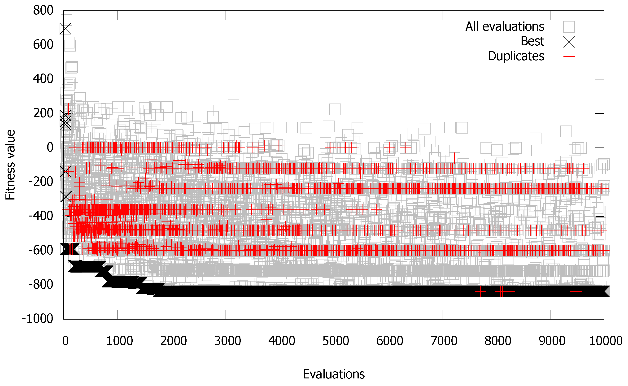
A better insight into the duplicates’ generation of a specific EA was obtained by observing the convergence graph of a particular independent run. Visualization of the convergence graph (black crosses) was enhanced with visualization of all generated solutions (gray squares) and duplicate solutions (red pluses). In particular, we would like to know how good the generated solutions (gray squares) were in terms of fitness, in which phases duplicates (red pluses) appeared (e.g., early in the search, when approaching local or global optima), and what was the convergence graph of the best solutions so far (black crosses). Such visualization helped us to understand better how specific EAs performed exploitation and exploration of the search space [14]. Namely, if the newly generated solutions (gray squares) were close to local optima or even to the best current solution (black crosses), then the EA was in the process of exploitation. On the other hand, if newly generated solutions (gray squares) were far from the best current solutions (black crosses), then the EA must be in the phase of exploration. On the graph, the x axis (horizontal) represents execution time represented by the number of evaluations and the y axis (vertical) the success of the algorithm represented by the fitness value. The graph has three types of data. The first type is all evaluations (gray squares), which represent all fitness evaluations and their values (10,000 of them). The second type of data represents the best solution found so far (best, black crosses) and describes the convergence of the algorithm. The last type of data represents the generated duplicate individuals (duplicates, red pluses). We need to note here that all solutions in the graph are presented by their fitness value (phenotype) and not by the actual result vector x (genotype).

Figure 4 represents one run of the ABC algorithm for $n=2$ and $Pr=6$ on the Sphere problem. From the graph (Figure 4), we can observe clearly two exploration phases of the ABC algorithm (all evaluations). The first exploration phase was in the interval from zero to ≈1500 evaluations, and the second started at ≈6000 and ended at 10,000 evaluations. The exploitation phase was in the interval from 1500 to 6000 (almost all generated solutions ended in the global optimum). Most duplicate individuals were generated in the global optimum in the interval from 4000 to 7000 evaluations when ABC was in the exploitation phase, whilst only a few duplicates were generated in the two exploration intervals.

5.1.2. Ackley Problem

The Ackley function problem has many local optima with a small basin of attraction and global optima with a large basin of attraction (Figure 5). The fitness value for the global optimum is zero. The minimization problem is characterized by the equation:

$$f\left(x\right)=-20exp\left(-0.2\sqrt{\frac{1}{n}\sum _{i=1}^n{x}_i^2}\right)-exp\left(\frac{1}{n}\sum _{i=1}^{n}cos2\pi x_i\right)+20+e$$

(4)

where $-32\le x_i\le 32$ and e is Euler’s number (≈2.7182818284).

Because of the local optima, it was expected that finding the global optimum would be harder than in the case of the Sphere problem, but due to the relatively small local optima basin of attraction compared to the global optima basin of attraction, EAs were able to make the exploration “jump” from local to global optimum.

The results are shown in

Table 5. Number of duplicate individuals’ evaluation for the Ackley problem.

EA	n	$\mathit{MFES}$	${\mathit{DBO}}_3$	${\mathit{DAll}}_3$	${\mathit{DBO}}_6$	${\mathit{DAll}}_6$	${\mathit{DBO}}_9$	${\mathit{DAll}}_9$	$\mathit{SR}$
ABC	2	10,000	$152.8$ $\pm 89.7$	$4254.2$ $\pm 173.2$	$103.5$ $\pm 52.2$	$2366.1$ $\pm 131.9$	$64.7$ $\pm 43.3$	$2322.9$ $\pm 169.9$	100
jDElscop	2	10,000	$68.4$ $\pm 51.5$	$6785.9$ $\pm 49.7$	$7.5$ $\pm 7.1$	$5175.0$ $\pm 129.7$	$6.6$ $\pm 2.9$	$4380.8$ $\pm 77.5$	100
TLBO	2	10,000	$54.2$ $\pm 36.7$	$1345.7$ $\pm 43.0$	$0.9$ $\pm 1.9$	$656.4$ $\pm 38.0$	$0.9$ $\pm 1.7$	$398.0$ $\pm 26.8$	100
GWO	2	10,000	$5.9$ $\pm 4.4$	$9586.4$ $\pm 38.4$	$0.0$ $\pm 0$	$9301.7$ $\pm 30.2$	$0.0$ $\pm 0$	$9064.3$ $\pm 25.2$	100
GOA	2	10,000	$627.5$ $\pm 476.1$	$1344.8$ $\pm 111.9$	$0.0$ $\pm 0$	$40.2$ $\pm 0.4$	$0.0$ $\pm 0$	$40.0$ $\pm 0$	96
ABC	10	30,000	$1348.1$ $\pm 454.4$	11,703.2 $\pm 581.2$	$211.6$ $\pm 96.1$	$7035.1$ $\pm 905.9$	$162.7$ $\pm 67.0$	$1431.2$ $\pm 357.0$	100
jDElscop	10	30,000	$62.3$ $\pm 23.1$	14,116.5 $\pm 113.9$	$1.1$ $\pm 0.9$	11,528.2 $\pm 259.9$	$1.4$ $\pm 1.3$	$8597.7$ $\pm 289.9$	100
TLBO	10	30,000	$660.9$ $\pm 182.3$	$1873.8$ $\pm 68.9$	$14.6$ $\pm 27.4$	$1158.9$ $\pm 49.3$	$0.0$ $\pm 0$	$799.0$ $\pm 33.2$	100
GWO	10	30,000	$11.6$ $\pm 14.7$	28,751.1 $\pm 101.2$	$0.0$ $\pm 0$	27,977.6 $\pm 120.3$	$0.0$ $\pm 0$	27,273.7 $\pm 77.5$	100
GOA	10	30,000	$1381.9$ $\pm 202.6$	$1381.9$ $\pm 202.6$	$27.0$ $\pm 9.5$	$30.0$ $\pm 0$	$30.0$ $\pm 0$	$30.0$ $\pm 0$	4
ABC	30	100,000	$6594.8$ $\pm 1276.2$	40,259.1 $\pm 606.3$	$493.8$ $\pm 142.0$	32,573.8 $\pm 2256.2$	$179.6$ $\pm 45.8$	12,076.3 $\pm 609.9$	100
jDElscop	30	100,000	$179.2$ $\pm 55.9$	48,279.1 $\pm 270.5$	$7.0$ $\pm 3.5$	43,431.3 $\pm 535.5$	$10.9$ $\pm 7.0$	38,226.1 $\pm 657.8$	100
TLBO	30	100,000	$3484.0$ $\pm 618.8$	$6357.3$ $\pm 138.6$	$5.2$ $\pm 6.9$	$4086.8$ $\pm 150.3$	$0.0$ $\pm 0$	$2994.6$ $\pm 115.6$	100
GWO	30	100,000	$8.0$ $\pm 7.0$	97,123.6 $\pm 195.9$	$0.0$ $\pm 0$	95,477.3 $\pm 99.1$	$0.0$ $\pm 0$	93,873.4 $\pm 122.6$	100
GOA	30	100,000	$5917.7$ $\pm 1329.9$	$5917.7$ $\pm 1329.9$	$70.0$ $\pm 0$	$70.0$ $\pm 0$	$40.0$ $\pm 0$	$40.0$ $\pm 0$	0

where we can observe that the number of duplicate individuals ($DBO$) was higher than for the Sphere function (Table 4). For example, the ABC algorithm for $n=10$ and $Pr=3$ had, on average, more than ≈$4\%$ of $DBO$; for $n=30$ and $Pr=3$ it had ≈$6\%$ of $DBO$. Indeed, among the selected EAs, the ABC algorithm had the highest number of $DBO$, showing that the proposed LTMA might be useful. The number of all duplicate individuals $DAll$ was similar (ABC around $\approx 40\%$) as in the case of the Sphere function (Table 4), indicating again that the number of $MFES$ could be lower. The $SR$ of $GOA$ showed again that this EA was not competitive for this kind of optimization problem. Around $60\%$ of duplicates would not be identified when only short term memory (current population) was used.

From the graph (Figure 6), we can again observe two exploration phases of ABC. Since the Ackley problem was harder than the Sphere problem, the first exploration phase of ABC was longer (up to 6000 evaluations) and generated more duplicates than the first exploration phase on the Sphere problem (Figure 4). Those duplicates were unnecessary, and it would be better if new unique solutions could be generated in an unexplored search space. In the exploitation phase (from 6000 to 8500 evaluations), many duplicates were actually at the global optimum. The ABC algorithm was no longer in the exploitation phase at ≈8500 evaluations, again generating a few duplicates.

5.1.3. Schwefel 2.26 Problem

The Schwefel 2.26 optimization problem had the most demanding fitness landscape among the three selected problems, with a lot of small and big basins of attraction (Figure 7). The minimization problem is characterized by the equation:

$$f\left(x\right)=-\sum _{i=1}^n\left(x_{i}sin\left(\sqrt{|x_i|}\right)\right)$$

(5)

where $-500\le x_i\le 500$.

The fitness value at the global optimum is $-418.982887272·n$.

From

Table 6. Number of duplicate individuals’ evaluation for the Schwefel 2.26 problem.

EA	n	$\mathit{MFES}$	${\mathit{DBO}}_3$	${\mathit{DAll}}_3$	${\mathit{DBO}}_6$	${\mathit{DAll}}_6$	${\mathit{DBO}}_9$	${\mathit{DAll}}_9$	$\mathit{SR}$
ABC	2	10,000	$1002.4$ $\pm 545.4$	$4069.6$ $\pm 134.1$	$935.2$ $\pm 164.9$	$3274.0$ $\pm 264.2$	$863.9$ $\pm 218.7$	$1762.8$ $\pm 339.5$	100
jDElscop	2	10,000	$284.3$ $\pm 92.0$	$5546.6$ $\pm 143.4$	$247.5$ $\pm 40.6$	$4408.1$ $\pm 123.8$	$246.3$ $\pm 44.0$	$338.1$ $\pm 183.1$	100
TLBO	2	10,000	$269.2$ $\pm 376.4$	$828.8$ $\pm 191.1$	$297.4$ $\pm 533.5$	$599.9$ $\pm 420.8$	$92.5$ $\pm 80.6$	$161.8$ $\pm 77.6$	90
GWO	2	10,000	$295.5$ $\pm 126.3$	$295.5$ $\pm 126.3$	$227.1$ $\pm 143.5$	$227.1$ $\pm 143.5$	$293.2$ $\pm 120.9$	$293.2$ $\pm 120.9$	10
GOA	2	10,000	$1223.5$ $\pm 969.8$	$1346.2$ $\pm 1065.0$	$1228.9$ $\pm 924.2$	$1326.3$ $\pm 993.2$	$1186.4$ $\pm 1093.0$	$1255.8$ $\pm 1149.2$	60
ABC	10	30,000	$4870.8$ $\pm 936.1$	$5688.0$ $\pm 494.5$	$2632.9$ $\pm 315.3$	$2759.3$ $\pm 273.8$	$2509.8$ $\pm 200.2$	$2552.8$ $\pm 219.6$	48
jDElscop	10	30,000	$175.5$ $\pm 33.5$	$7190.8$ $\pm 358.6$	$176.1$ $\pm 36.3$	$1518.0$ $\pm 355.0$	$185.5$ $\pm 36.1$	$187.9$ $\pm 35.7$	100
TLBO	10	30,000	$79.4$ $\pm 47.3$	$79.4$ $\pm 47.3$	$1.0$ $\pm 1.2$	$1.0$ $\pm 1.2$	$2.7$ $\pm 7.2$	$2.7$ $\pm 7.2$	0
GWO	10	30,000	$0.0$ $\pm 0$	$0.0$ $\pm 0$	$0.0$ $\pm 0$	$0.0$ $\pm 0$	$0.0$ $\pm 0$	$0.0$ $\pm 0$	0
GOA	10	30,000	$150.4$ $\pm 1.8$	$150.4$ $\pm 1.8$	$30.0$ $\pm 0$	$30.0$ $\pm 0$	$0.0$ $\pm 0$	$0.0$ $\pm 0$	0
ABC	30	100,000	18,168.4 $\pm 1583.2$	18,168.4 $\pm 1583.2$	$7175.4$ $\pm 671.3$	$7175.4$ $\pm 671.3$	$6155.2$ $\pm 759.3$	$6155.2$ $\pm 759.3$	0
jDElscop	30	100,000	$640.2$ $\pm 72.6$	24,746.7 $\pm 863.2$	$611.8$ $\pm 51.2$	$2920.5$ $\pm 208.1$	$643.0$ $\pm 31.8$	$645.2$ $\pm 32.5$	100
TLBO	30	100,000	$213.0$ $\pm 123.1$	$213.0$ $\pm 123.1$	$5.1$ $\pm 4.2$	$5.1$ $\pm 4.2$	$0.1$ $\pm 0.3$	$0.1$ $\pm 0.3$	0
GWO	30	100,000	$0.0$ $\pm 0$	$0.0$ $\pm 0$	$0.0$ $\pm 0$	$0.0$ $\pm 0$	$0.0$ $\pm 0$	$0.0$ $\pm 0$	0
GOA	30	100,000	$392.5$ $\pm 65.0$	$392.5$ $\pm 65.0$	$40.0$ $\pm 0$	$40.0$ $\pm 0$	$0.0$ $\pm 0$	$0.0$ $\pm 0$	0

, we can observe that the number of duplicate individuals before the global optimum ($DBO$) increased in comparison with the Sphere or Ackley problems (Table 4 and Table 5). Again, ABC generated the most $DBO$ among the selected EAs (more than $10\%$), although it was the runner-up regarding $SR$, where jDElscop had the best performance. It is interesting that the number of duplicates $DAll$ was not much higher than $DBO$, indicating that the most duplicates were actually sub-optimal solutions. Around $75\%$ of duplicates would not be identified when only short-term memory (current population) was used.

The graph on Figure 8 for ABC indicates that duplicate individuals were generated throughout the whole optimization process. Most duplicates were generated at six different fitness values (red stripes on the graph). These were the values of the local optima. About $10\%$ of all generated solutions were $DBO$. Clearly, re-visited solutions would be better spent on exploring new regions. The proposed LTMA would again be very beneficial.

5.2. Experiment II: CEC-2015 Benchmark

In this experiment, we wanted to test selected EAs on benchmarks that are often used to compare EAs. The focus of the experiment was not just on the number of generated duplicate individuals ($DBO$ and $DAll$), but also on the time t needed to execute the optimization (a single independent run presented in seconds). For this, we used the $LTM{A}_t$ scenario. Furthermore, we were interested in how the convergence of an EA could be improved by replacing duplicates (before their fitness function was re-evaluated) with non-revisited solutions. In this scenario, $LTM{A}_e$, each EA was run until $MFES$ different solutions were checked. We also report the percentage of runs where the final solution was improved. This scenario showed directly the impact of the LTMA on the improvement of the EA’s convergence.

The execution time of an experiment depends on the running environment: software and hardware. The experiment was executed on a computer with Intel(R) Core(TM) i7-7500U CPU @ 2.7 GHz with 16 GB RAM and the Windows 10 64-bit operating system. The execution was not multi-core CPU optimized.

For this experiment, we selected the ABC algorithm and the most successful algorithm from previous experiments: jDElscop. EA control parameters were the same as in Experiment I. For the benchmark, we selected the CEC-2015 benchmark from the Competition on Real-Parameter Single Objective Optimization [62]. The benchmark has 10 different minimization problems (from $F01$ to $F10$). For our scenario, we set $n=10$ and $MFES=$ 100,000. The global optimum for problem $F01$ was 100, for $F02$ 200, ..., and for $F10$ 1000. LTMA was also compared to a standard version (i.e., without LTMA), and its results are shown in the last two columns in

Table 7. ABC algorithm on CEC-2015 with $LTM{A}_t$.

Pro.	${\mathit{DBO}}_6$	${\mathit{DAll}}_6$	${\mathit{Fit}}_6$	${\mathit{t}}_6$	${\mathit{DBO}}_9$	${\mathit{DAll}}_9$	${\mathit{Fit}}_9$	${\mathit{t}}_9$	Fit	t
$F01$	$5033.4$ $\pm 816.4$	$5033.4$ $\pm 816.4$	$7766.0$ $\pm 6064.7$	$0.3$ $\pm 0.2$	$4867.1$ $\pm 872.8$	$4867.1$ $\pm 872.8$	$7152.7$ $\pm 5733.5$	$0.3$ $\pm 0.1$	$7630.0$ $\pm 5881.4$	$0.1$ $\pm 0.1$
$F02$	26,711.8 $\pm 806.8$	26,711.8 $\pm 806.8$	13,710.4 $\pm 3254.7$	$0.2$ $\pm 0.0$	26,574.3 $\pm 672.4$	26,574.3 $\pm 672.4$	12,868.0 $\pm 3034.8$	$0.2$ $\pm 0.0$	12,971.5 $\pm 3574.3$	$0.1$ $\pm 0.0$
$F03$	23,124.3 $\pm 844.1$	23,124.3 $\pm 844.1$	$304.8$ $\pm 0.8$	$\mathbf{11.6}$ $\pm 0.4$	23,058.7 $\pm 1019.6$	23,058.7 $\pm 1019.6$	$304.7$ $\pm 0.8$	$\mathbf{11.6}$ $\pm 0.3$	$304.7$ $\pm 1.0$	$\mathbf{14.8}$ $\pm 0.3$
$F04$	16,360.0 $\pm 5393.9$	19,455.2 $\pm 2311.9$	$400.2$ $\pm 0.5$	$0.3$ $\pm 0.0$	$4668.0$ $\pm 1782.0$	$4998.3$ $\pm 1648.0$	$401.3$ $\pm 6.2$	$0.4$ $\pm 0.1$	$400.1$ $\pm 0.1$	$0.2$ $\pm 0.0$
$F05$	22,551.8 $\pm 759.8$	22,551.8 $\pm 759.8$	$500.5$ $\pm 0.1$	$\mathbf{2.4}$ $\pm 0.0$	22,698.8 $\pm 730.4$	22,698.8 $\pm 730.4$	$500.5$ $\pm 0.1$	$\mathbf{2.4}$ $\pm 0.0$	$500.5$ $\pm 0.1$	$\mathbf{2.8}$ $\pm 0.0$
$F06$	$2195.1$ $\pm 277.6$	$2209.1$ $\pm 215.6$	$600.2$ $\pm 0.0$	$0.2$ $\pm 0.0$	$2194.9$ $\pm 196.5$	$2194.9$ $\pm 196.5$	$600.2$ $\pm 0.0$	$0.2$ $\pm 0.0$	$600.2$ $\pm 0.0$	$0.1$ $\pm 0.0$
$F07$	$587.2$ $\pm 140.7$	$632.9$ $\pm 66.4$	$700.1$ $\pm 0.0$	$0.2$ $\pm 0.0$	$630.5$ $\pm 96.5$	$641.6$ $\pm 69.4$	$700.2$ $\pm 0.0$	$0.3$ $\pm 0.0$	$700.1$ $\pm 0.0$	$0.1$ $\pm 0.0$
$F08$	$1413.4$ $\pm 238.1$	$1413.4$ $\pm 238.1$	$801.1$ $\pm 0.3$	$0.3$ $\pm 0.0$	$1413.0$ $\pm 225.7$	$1413.0$ $\pm 225.7$	$801.1$ $\pm 0.3$	$0.3$ $\pm 0.0$	$801.2$ $\pm 0.3$	$0.1$ $\pm 0.0$
$F09$	21,728.5 $\pm 965.0$	21,728.5 $\pm 965.0$	$903.0$ $\pm 0.2$	$0.3$ $\pm 0.0$	21,908.3 $\pm 1044.2$	21,908.3 $\pm 1044.2$	$903.0$ $\pm 0.2$	$0.3$ $\pm 0.0$	$903.0$ $\pm 0.2$	$0.1$ $\pm 0.0$
$F10$	22,954.7 $\pm 1106.1$	22,954.7 $\pm 1106.1$	11,114.8 ±11,329.6	$0.3$ $\pm 0.0$	22,803.2 $\pm 1073.5$	22,803.2 $\pm 1073.5$	10,484.4 $\pm 7761.3$	$0.4$ $\pm 0.0$	11,546.5 $\pm 9585.6$	$0.2$ $\pm 0.0$

and

Table 8. jDElscop algorithm on CEC-2015 with $LTM{A}_t$.

Pro.	${\mathit{DBO}}_6$	${\mathit{DAll}}_6$	${\mathit{Fit}}_6$	${\mathit{t}}_6$	${\mathit{DBO}}_9$	${\mathit{DAll}}_9$	${\mathit{Fit}}_9$	${\mathit{t}}_9$	Fit	t
$F01$	$34.0$ $\pm 13.6$	15,142.5 $\pm 1852.6$	$100.0$ $\pm 0.0$	$0.3$ $\pm 0.1$	$36.6$ $\pm 14.9$	$3897.2$ $\pm 4690.9$	$100.0$ $\pm 0.0$	$0.3$ $\pm 0.1$	$100.0$ $\pm 0.0$	$0.2$ $\pm 0.1$
$F02$	$93.4$ $\pm 41.4$	$5949.0$ $\pm 4809.9$	$200.0$ $\pm 0.0$	$0.3$ $\pm 0.0$	$90.0$ $\pm 36.6$	$110.2$ $\pm 37.6$	$200.0$ $\pm 0.0$	$0.3$ $\pm 0.0$	$200.0$ $\pm 0.0$	$0.2$ $\pm 0.1$
$F03$	$5688.5$ $\pm 6817.4$	16,487.8 $\pm 3251.6$	$300.6$ $\pm 1.1$	$\mathbf{12.6}$ $\pm 0.5$	$4085.7$ $\pm 5119.1$	12,137.0 $\pm 2988.1$	$300.6$ $\pm 1.1$	$\mathbf{13.4}$ $\pm 0.5$	$300.5$ $\pm 0.9$	$\mathbf{15.2}$ $\pm 0.6$
$F04$	$3234.2$ $\pm 6496.9$	20,848.0 $\pm 1255.0$	$400.0$ $\pm 0.0$	$0.4$ $\pm 0.0$	$463.1$ $\pm 178.5$	$509.4$ $\pm 175.0$	$400.2$ $\pm 0.7$	$0.5$ $\pm 0.0$	$400.8$ $\pm 4.2$	$0.3$ $\pm 0.0$
$F05$	13,453.9 $\pm 4443.0$	13,500.5 $\pm 4355.1$	$500.7$ $\pm 0.3$	$\mathbf{2.7}$ $\pm 0.1$	12,857.5 $\pm 4563.3$	12,892.5 $\pm 4518.8$	$500.7$ $\pm 0.3$	$\mathbf{2.7}$ $\pm 0.1$	$500.8$ $\pm 0.3$	$\mathbf{2.9}$ $\pm 0.0$
$F06$	$7478.5$ $\pm 5840.1$	$9709.3$ $\pm 5334.7$	$600.1$ $\pm 0.0$	$0.3$ $\pm 0.0$	$7785.8$ $\pm 5760.9$	$9200.3$ $\pm 5489.0$	$600.1$ $\pm 0.0$	$0.3$ $\pm 0.0$	$600.2$ $\pm 0.0$	$0.2$ $\pm 0.0$
$F07$	$7450.6$ $\pm 5626.3$	$9762.0$ $\pm 4877.0$	$700.1$ $\pm 0.0$	$0.3$ $\pm 0.0$	$6967.1$ $\pm 5583.3$	$8991.2$ $\pm 4998.2$	$700.1$ $\pm 0.0$	$0.3$ $\pm 0.1$	$700.1$ $\pm 0.0$	$0.2$ $\pm 0.0$
$F08$	$6960.2$ $\pm 4754.2$	$6960.2$ $\pm 4754.2$	$801.1$ $\pm 0.3$	$0.4$ $\pm 0.0$	$6798.2$ $\pm 6261.3$	$6798.2$ $\pm 6261.3$	$801.2$ $\pm 0.4$	$0.4$ $\pm 0.0$	$801.2$ $\pm 0.4$	$0.2$ $\pm 0.0$
$F09$	$8608.7$ $\pm 4361.9$	$8608.7$ $\pm 4361.9$	$902.5$ $\pm 0.4$	$0.4$ $\pm 0.0$	$7563.9$ $\pm 5059.4$	$7563.9$ $\pm 5059.4$	$902.5$ $\pm 0.4$	$0.4$ $\pm 0.0$	$902.5$ $\pm 0.4$	$0.2$ $\pm 0.0$
$F10$	$130.3$ $\pm 38.3$	$130.3$ $\pm 38.3$	$1026.4$ $\pm 37.7$	$0.5$ $\pm 0.0$	$125.4$ $\pm 37.4$	$125.4$ $\pm 37.4$	$1038.1$ $\pm 47.1$	$0.5$ $\pm 0.0$	$1037.3$ $\pm 46.2$	$0.3$ $\pm 0.0$

.

The number of different configurations (10 different problems, different precisions, 2 EAs, 2 scenarios: $LT{M}_t$ and $LT{M}_e$) in total was 120, each of which was performed on 100 independent runs.

5.2.1. Scenario $LTM{A}_t$

In this experiment, we measured how much CPU time could be saved by not re-evaluating the fitness of revisited solutions (i.e., the fitness value was just read from the LTMA module).

From the results in Table 7 and Table 8, we can observe that the ratio of generated duplicate individuals was surprisingly high. The reason for this was that the problems in the benchmark were difficult (e.g., many different local optima). In the case of ABC, more than $20\%$ of the generated solutions were $DBO$ (e.g., for $F02$, $F03$, $F05$, $F09$, and $F10$); whilst jDElscop generated more than $5\%$$DBO$ for problems $F05$–$F09$. Around $90\%$ of duplicates would not be identified when only short term memory (current population) was used.

Although the number of $DBO$ was high, the speedup using LTMA was not achieved in most cases. The reason was that for the most problems ($F01$–$F10$, except $F03$ and $F05$), fitness evaluations were fast and took, on average, less than $0.2$ s for one optimization run; whilst identifying duplicates took on average $0.15\pm 0.05$ s. In such cases, the use of LTMA was not justified. It should be noted that ABC did not find a suitable solution for problems $F01,F02$, and $F10$, whilst jDElscop did.

$F03$ and $F05$ were more difficult problems that could clearly show the profits of applying LTMA (see the bold values in Table 7 and Table 8). When LTMA was not applied, these two problems took $14.8\pm 0.3$ s and $2.8\pm 0.0$ s (Table 7), respectively. Yet, with LTMA, the execution times taken by ABC dropped to $11.6\pm 0.3$ s and $2.4\pm 0.0$ s, respectively. Equivalently, this means that LTMA increased speedup by $1.28$ for the $F03$ problem and by $1.16$ for the $F05$ problem. From Table 7, we noticed that precisions did not play an important role for these two problems: There was almost no difference between scenarios with precision of six and nine.

Since generating duplicates was algorithm dependent, LTMA driven profits were different between ABC and jDElscop. Table 8 shows that $F03$ took $15.2\pm 0.6$ s on average, and $F05$ spent $2.7\pm 0.1$ s. On average, jDElscop with LTMA improved the execution time, expressed as speedup, $1.16\times$ for the $F03$ problem and $1.07$ for the $F05$ problem. Overall, we can expect increased speedup and faster EA execution by not re-evaluating duplicates for time consuming problems. In such cases, termination based on the maximum CPU time should also produce equal or better results using the LTMA approach.

5.2.2. Scenario $LTM{A}_e$

In this experiment, we tested the $LTM{A}_e$ scenario. Namely, when a duplicate was identified, but not re-evaluated, it was replaced with a new non-revisited individual. With additional search points, it was expected to obtain better or equal results. To present possible benefits better, we counted runs where solutions were improved. They are presented as the percentage of improved runs (B) (

Table 9. ABC algorithm on CEC-2015 with $LTM{A}_e$.

Pro.	${\mathit{DBO}}_6$	${\mathit{DAll}}_6$	${\mathit{Fit}}_6$	${\mathit{t}}_6$	${\mathit{B}}_6$	${\mathit{DBO}}_9$	${\mathit{DAll}}_9$	${\mathit{Fit}}_9$	${\mathit{t}}_9$	${\mathit{B}}_9$
$F01$	$5372.3$ $\pm 911.4$	$5372.3$ $\pm 911.4$	$7471.8$ $\pm 6093.4$	$0.3$ $\pm 0.2$	26%	$5192.2$ $\pm 981.3$	$5192.2$ $\pm 981.3$	$6971.2$ $\pm 5727.9$	$0.3$ $\pm 0.1$	25%
$F02$	36,731.3 $\pm 1296.9$	36,731.3 $\pm 1296.9$	12,767.4 $\pm 2991.4$	$0.3$ $\pm 0.0$	23%	36,503.8 $\pm 1069.2$	36,503.8 $\pm 1069.2$	12,019.9 $\pm 2916.2$	$0.4$ $\pm 0.0$	29%
$F03$	30,440.7 $\pm 1316.2$	30,440.7 $\pm 1316.2$	$304.6$ $\pm 0.9$	$15.2$ $\pm 0.6$	25%	30,172.2 $\pm 1532.7$	30,172.2 $\pm 1532.7$	$304.5$ $\pm 0.9$	$15.1$ $\pm 0.3$	40%
$F04$	18,153.2 $\pm 6884.0$	23,244.3 $\pm 3216.3$	$400.1$ $\pm 0.3$	$0.5$ $\pm 0.0$	60%	$4797.5$ $\pm 2010.3$	$5198.3$ $\pm 1862.7$	$401.3$ $\pm 6.2$	$0.5$ $\pm 0.1$	51%
$F05$	29,324.9 $\pm 1182.6$	29,324.9 $\pm 1182.6$	$500.5$ $\pm 0.1$	$3.1$ $\pm 0.0$	29%	29,554.8 $\pm 1137.6$	29,554.8 $\pm 1137.6$	$500.5$ $\pm 0.1$	$3.1$ $\pm 0.0$	29%
$F06$	$2243.9$ $\pm 284.7$	$2258.4$ $\pm 220.8$	$600.2$ $\pm 0.0$	$0.3$ $\pm 0.0$	2%	$2244.8$ $\pm 203.4$	$2244.8$ $\pm 203.4$	$600.2$ $\pm 0.0$	$0.3$ $\pm 0.0$	2%
$F07$	$590.0$ $\pm 141.9$	$636.3$ $\pm 67.1$	$700.1$ $\pm 0.0$	$0.3$ $\pm 0.0$	0%	$634.6$ $\pm 97.3$	$645.8$ $\pm 69.9$	$700.2$ $\pm 0.0$	$0.3$ $\pm 0.0$	2%
$F08$	$1433.1$ $\pm 244.4$	$1433.1$ $\pm 244.4$	$801.1$ $\pm 0.3$	$0.3$ $\pm 0.0$	12%	$1432.5$ $\pm 230.5$	$1432.5$ $\pm 230.5$	$801.1$ $\pm 0.3$	$0.3$ $\pm 0.0$	24%
$F09$	27,947.6 $\pm 1392.8$	27,947.6 $\pm 1392.8$	$903.0$ $\pm 0.2$	$0.4$ $\pm 0.1$	36%	28,205.2 $\pm 1600.9$	28,205.2 $\pm 1600.9$	$903.0$ $\pm 0.2$	$0.4$ $\pm 0.0$	40%
$F10$	30,065.2 $\pm 1706.8$	30,065.2 $\pm 1706.8$	$9306.8$ $\pm 7878.0$	$0.5$ $\pm 0.0$	21%	29,929.6 $\pm 1720.9$	29,929.6 $\pm 1720.9$	$9571.1$ $\pm 7387.4$	$0.5$ $\pm 0.0$	12%

and

Table 10. jDElscop algorithm on CEC-2015 with $LTM{A}_e$.

Pro.	${\mathit{DBO}}_6$	${\mathit{DAll}}_6$	${\mathit{Fit}}_6$	${\mathit{t}}_6$	${\mathit{B}}_6$	${\mathit{DBO}}_9$	${\mathit{DAll}}_9$	${\mathit{Fit}}_9$	${\mathit{t}}_9$	${\mathit{B}}_9$
$F01$	$34.0$ $\pm 13.6$	36,269.0 $\pm 5838.1$	$100.0$ $\pm 0.0$	$0.4$ $\pm 0.1$	5%	$36.6$ $\pm 14.9$	$8772.1$ ±10,835.2	$100.0$ $\pm 0.0$	$0.4$ $\pm 0.1$	48%
$F02$	$93.4$ $\pm 41.4$	12,908.8 ±10,847.5	$200.0$ $\pm 0.0$	$0.4$ $\pm 0.0$	41%	$90.0$ $\pm 36.6$	$110.3$ $\pm 37.6$	$200.0$ $\pm 0.0$	$0.3$ $\pm 0.0$	89%
$F03$	12,208.1 ±15,016.7	35,757.9 $\pm 6807.2$	$300.6$ $\pm 1.1$	$15.2$ $\pm 0.3$	2%	$8609.8$ ±11,189.7	26,191.1 $\pm 6487.8$	$300.6$ $\pm 1.1$	$15.3$ $\pm 0.3$	1%
$F04$	$4544.2$ ±11,004.4	44,841.8 $\pm 2746.7$	$400.0$ $\pm 0.0$	$0.6$ $\pm 0.0$	17%	$463.2$ $\pm 178.6$	$510.3$ $\pm 175.3$	$400.2$ $\pm 0.7$	$0.5$ $\pm 0.0$	0%
$F05$	26,990.6 ±12,096.8	27,169.1 ±11,827.0	$500.6$ $\pm 0.3$	$3.1$ $\pm 0.0$	54%	24,287.9 ±12,501.4	24,468.8 ±12,314.9	$500.7$ $\pm 0.3$	$3.1$ $\pm 0.0$	51%
$F06$	15,763.2 ±15,183.5	21,721.5 ±14,162.7	$600.1$ $\pm 0.0$	$0.4$ $\pm 0.0$	12%	16,266.4 ±14,745.1	20,168.4 ±14,010.7	$600.1$ $\pm 0.1$	$0.4$ $\pm 0.1$	11%
$F07$	15,509.7 ±14,363.5	21,797.1 ±13,112.1	$700.1$ $\pm 0.0$	$0.4$ $\pm 0.0$	15%	14,768.1 ±14,181.0	19,777.9 ±13,410.9	$700.1$ $\pm 0.0$	$0.4$ $\pm 0.1$	14%
$F08$	13,746.8 ±10,436.1	13,746.8 ±10,436.1	$801.0$ $\pm 0.3$	$0.4$ $\pm 0.0$	63%	14,948.1 ±21,325.4	14,948.1 ±21,325.4	$801.1$ $\pm 0.4$	$0.4$ $\pm 0.1$	39%
$F09$	14,896.3 ±10,625.5	14,896.3 ±10,625.5	$902.4$ $\pm 0.4$	$0.4$ $\pm 0.0$	66%	12,068.1 ±15,081.8	12,068.1 ±15,081.8	$902.4$ $\pm 0.4$	$0.5$ $\pm 0.1$	55%
$F10$	$130.4$ $\pm 38.7$	$130.4$ $\pm 38.7$	$1026.4$ $\pm 37.7$	$0.5$ $\pm 0.0$	95%	$125.5$ $\pm 37.4$	$125.5$ $\pm 37.4$	$1038.1$ $\pm 47.1$	$0.5$ $\pm 0.0$	94%

).

How much the algorithm gained with additional evaluations was problem and algorithm dependent. In the case of the ABC algorithm, most improvements were shown on problem $F04$, where, in more than $50\%$ of runs, the results were improved, with almost no improvements in the case of problem $F07$ (Table 9). The jDElscop algorithm gained the most in the case of problems $F02$ and $F10$, where around $90\%$ of all runs resulted in optimal solution improvement (Table 10). Overall, with the proposed LTMA approach, the search space would be explored better and exploited since duplicate individuals were eliminated. In most cases, a better solution was found.

5.3. Experiment III: Real-World Problem

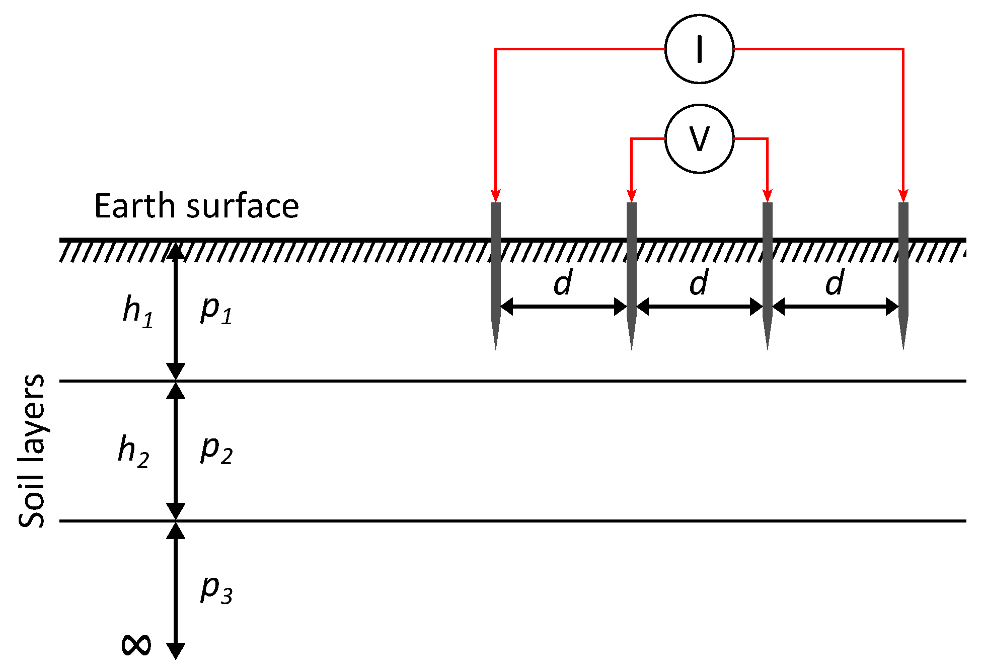
The real-world optimization problem we used in our experiments dealt with searching for soil models’ parameters, namely the thicknesses of the soil layers and their resistances [63]. It was assumed that the soil was homogeneous within each layer. In our calculations, we used the three-layer soil model, which was shown to obtain the best results in [64]. The three-layered model is shown in Figure 9, where $h_1$ and $h_2$ are the thicknesses of the soil layers and $p_1$ to $p_3$ are specific soil resistances of the soil layers. The obtained soil parameters based on the soil model were used in the Finite Element Method (FEM) for proper dimensioning of the grounding systems. Grounding systems play an important role in protecting people and devices in cases of defects in electro-energetic systems or lightning strikes. In order to determine the soil’s parameters, information is required regarding the soil’s structure in the surroundings of the grounding system. These data were obtained with different measuring methods. In our experiments, we used three different measured datasets (problem instances $TE1$, $TE2$, and $TE3$) obtained with the most commonly used Wenner four-electrode method [65]. In the Wenner method, four electrodes are inserted into the earth at equal spacings d (Figure 9).

The earth’s apparent resistivity is then measured according to:

$$p_d^m=\frac{2\pi dU}{I}$$

(6)

where d is the distance between two consecutive electrodes, I is the current injected between the two outer electrodes, and U is the voltage measured between the two inner electrodes. Based on the same definition, the analytical expression for apparent resistivity is calculated as:

$$p_d^c=p_1\left\{1+2d{\int }_0^{\infty }f\left(\lambda \right)\left[J_0\left(\lambda d\right)-J_0\left(2\lambda d\right)\right]d\lambda \right\}$$

(7)

where $p_1$ is the specific resistivity of the first soil layer and $J_0$ is the zero order Bessel’s function of the first kind, calculated using Equation (8).

$$f\left(\lambda \right)={\alpha }_1\left(\lambda \right)-1$$

(8)

For the three-layered soil model, ${\alpha }_1$ was calculated with the equations presented in Equation (9).

$$\begin{array}{cc}{K}_1\left(\lambda \right)=\frac{p_2{\alpha }_2\left(\lambda \right)-p_1}{p_2{\alpha }_2\left(\lambda \right)+p_1};& {\alpha }_1\left(\lambda \right)=1+\frac{2K_1{e}^{-2\lambda h_1}}{1-K_1{e}^{-2\lambda h_1}}\\ K_2\left(\lambda \right)=\frac{p_3-p_2}{p_3+p_2};& {\alpha }_2\left(\lambda \right)=1+\frac{2K_2{e}^{-2\lambda h_2}}{1-K_2{e}^{-2\lambda h_2}}\end{array}$$

(9)

A numerical integration was adapted for the integration. Infinity was replaced with a large value, denoted by ${\lambda }_{max}$, and was set according to [66]. The goal of the optimization was to find the soil parameters that best fit the measurement data. The fitness function was defined as:

$$F_{fitness}=\frac{1}{n}\sum _{i=1}^n\left|\frac{p_i^c-p_i^m}{p_i^m}\right|·100(\%)$$

(10)

where $p_i^m$ are the measured and $p_i^c$ the calculated values of apparent resistivity, respectively. n is the number of measured points.

For the experiment, we set $MFES=$ 20,000. For EA assistance (ABC, jDElscop), we selected $LTM{A}_t$. Every experiment was repeated 50 times. In this section, we had 12 different configurations (3 problem instances, 3 scenarios, and 2 EAs).

In the case of the ABC algorithm ($TE1$ problem), there were ≈7000 duplicate individuals, which was $35\%$ and was unexpectedly high, and it was similar for the $TE2$ and $TE3$ problems (

Table 11. Optimization of soil problem with the ABC and jDElscop algorithms.

EA	Pro.	${\mathit{DBO}}_6$	${\mathit{DAll}}_6$	${\mathit{Fit}}_6$	${\mathit{t}}_6$	${\mathit{DBO}}_9$	${\mathit{DAll}}_9$	${\mathit{Fit}}_9$	${\mathit{t}}_9$	$\mathit{Fit}$	t
ABC	$TE1$	$7284.7$ $\pm 434.3$	$7284.7$ $\pm 434.3$	$1.2$ $\pm 0.2$	$71.7$ $\pm 14.0$	$7206.7$ $\pm 549.7$	$7206.7$ $\pm 549.7$	$1.2$ $\pm 0.3$	$69.0$ $\pm 12.3$	$1.2$ $\pm 0.3$	$126.3$ $\pm 17.0$
ABC	$TE2$	$5545.6$ $\pm 437.3$	$5545.6$ $\pm 437.3$	$3.1$ $\pm 0.5$	$41.4$ $\pm 9.8$	$5481.2$ $\pm 367.2$	$5481.2$ $\pm 367.2$	$3.3$ $\pm 0.9$	$35.8$ $\pm 10.8$	$3.2$ $\pm 1.2$	$55.1$ $\pm 15.0$
ABC	$TE3$	$6033.4$ $\pm 753.1$	$6033.4$ $\pm 753.1$	$2.0$ $\pm 0.1$	$76.8$ $\pm 23.1$	$6387.0$ $\pm 968.8$	$6387.0$ $\pm 968.8$	$2.0$ $\pm 0.1$	$66.8$ $\pm 19.5$	$2.1$ $\pm 0.1$	$108.4$ $\pm 34.9$
jDElscop	$TE1$	$278.3$ $\pm 317.5$	$278.3$ $\pm 317.5$	$1.2$ $\pm 0.4$	$31.8$ $\pm 32.2$	$188.3$ $\pm 102.1$	$188.3$ $\pm 102.1$	$1.1$ $\pm 0.0$	$24.9$ $\pm 2.0$	$1.1$ $\pm 0.0$	$27.3$ $\pm 2.8$
jDElscop	$TE2$	$349.0$ $\pm 663.8$	$349.0$ $\pm 663.8$	$4.5$ $\pm 2.2$	$13.5$ $\pm 5.4$	$446.7$ $\pm 642.2$	$446.7$ $\pm 642.2$	$4.9$ $\pm 2.1$	$12.3$ $\pm 5.0$	$4.8$ $\pm 2.0$	$13.3$ $\pm 5.7$
jDElscop	$TE3$	$4709.4$ $\pm 430.0$	$4709.4$ $\pm 430.0$	$2.3$ $\pm 0.2$	$25.5$ $\pm 32.1$	$3752.5$ $\pm 656.4$	$3752.5$ $\pm 656.4$	$2.8$ $\pm 2.0$	$29.5$ $\pm 40.0$	$2.7$ $\pm 2.3$	$48.3$ $\pm 65.7$

). In the case of the jDElscop algorithm, the percentage of duplicates was much lower, but, in the case of the $TE3$ problem, the duplicate percentage was still high at $20\%$.

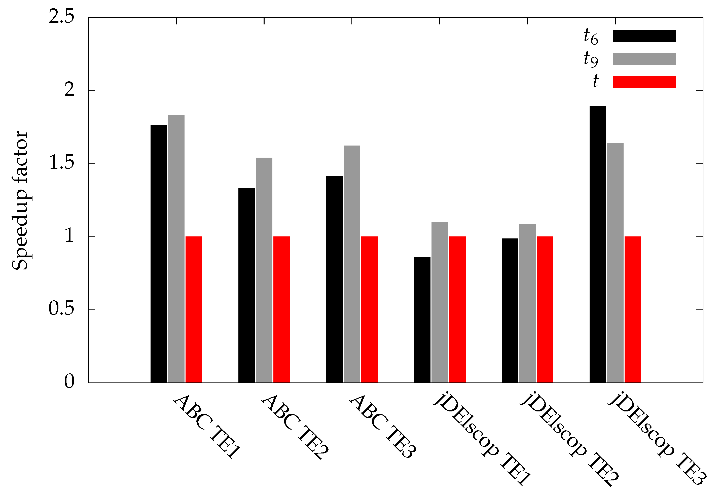
The execution time of a single independent run (t) in the case of the real-world can fluctuate greatly. On average, for the ($TE1$, $TE2$, and $TE3$) optimization process of a singe run for the ABC algorithm, we needed $47.45$ s for $Pr=6$, $42.91$ s for $Pr=9$, and $72.43$ s without $LTM{A}_t$ (Table 11). We obtained speedups: $1.53$ for $Pr=6$ and $1.69$ for $Pr=9$. In the case of the jDElscop algorithm, the number of generated duplicate individuals was lower than in the case of the ABC algorithm. On average, for the ($TE1$, $TE2$ and $TE3$) optimization process of a singe run, we needed $17.68$ s for $Pr=6$, $16.69$ s for $Pr=9$, and $22.23$ s without $LTM{A}_t$. We obtained speedups: $1.26$ for $Pr=6$ and $1.33$ for $Pr=9$ (Table 11).

We can observe from Figure 10 that with, the LTMA speedup for real-world problems can be substantial (around 50%).

6. Conclusions

To investigate the generation of duplicate individuals over the whole evolutionary process, we conducted more than 250 different configurations, divided between three experiments, during which we analyzed how much profit we could gain by not re-evaluating duplicate individuals (their fitness values can just be accessed from the memory) and how many new solutions could be generated when eliminating duplicates completely. The main conclusions of this study are:

• For identifying duplicate individuals (re-visited solutions), it is not enough to use a short term memory (current population). The experiments showed that between 50% and 90% of duplicates would not be discovered without long term memory (all generated solutions in the whole evolutionary process).
• Current achievements in hardware allowed us to store all solutions (phenotype and genotype) in the computer’s RAM, where we can identify duplicate individuals easily.
• A speedup of $10\%$ or more can be achieved for hard real-world problems where fitness evaluations are costly, simply by not re-evaluating duplicates (when at least $10\%$ of duplicates are generated). In the case of the soil model problem, ABC generated around $35\%$ duplicate individuals, and, with the proposed LTMA, a speedup of $1.59$ was achieved.
• Better convergence can be achieved when duplicate individuals are replaced with non-revisited individuals. In such a manner, the search space could be explored and exploited better.
• A long term memory can be attached in a uniform way to existing EAs.

Please note that the primary goal of this study was to show how researchers/practitioners may increase/improve their algorithm’s efficiency motivated by detailed analyses obtained from LTMA. Our focus was not to compare the performance of the selected algorithms, which has been done intensively in the research community. Studying an algorithm without an in-depth analysis may deceive us into drawing an inaccurate conclusion on the superiority of one algorithm over another. For example, one might conclude that the ABC algorithm was inferior, because it created more duplicates than the jDElscop algorithm and in most scenarios produced worse results. However, this is not necessarily the case. The ABC algorithm had an innovative mechanism for maintaining diversity using the “limit” parameter, which was, in our implementation, set indirectly by control parameters. Conversely, the jDElscop algorithm used the mechanism of population reduction, which released selection pressure. Both, consequently, influenced the number of duplicates [19]. In conclusion, because the mechanisms of both algorithms depended on the control parameters, one cannot draw conclusions about the superiority of individual algorithms based merely on this study.

EAs are very convenient for black-box optimization where we do not know much about a problem’s characteristics. We are convinced that the long term memory module can be an important contribution in the overall optimization’s success. EA users should be informed about how many duplicate solutions have been generated and how the search spaces has been explored and exploited. The search should not be completely blind. In our future work, we will investigate how visual analytics can help EA researchers and users to understand EA’s inner workings better.

Last but not least, the suggested LTMA did not add much complexity to the EAs’ implementation, and it helped reduce uncertainties about stochastic optimization efficiency by preventing the evaluation of redundant solutions. Therefore, it should be used widely in computationally demanding optimizations. Note that the proposed approach is not suitable for noisy and dynamic problems, where an individual’s fitness changes frequently over time.

References

- Eiben, A.G.; Smith, J.E. Introduction to Evolutionary Computing; Springer: Heidelberg, Germany, 2015. [Google Scholar]
- Karaboga, D.; Basturk, B. On the performance of artificial bee colony (ABC) algorithm. Appl. Soft Comput. 2008, 8, 687–697. [Google Scholar] [CrossRef]
- Dorigo, M.; Gambardella, L.M. Ant colony system: A cooperative learning approach to the traveling salesman problem. IEEE Trans. Evol. Comput. 1997, 1, 53–66. [Google Scholar] [CrossRef]
- Saremi, S.; Mirjalili, S.; Lewis, A. Grasshopper optimisation algorithm: Theory and application. Adv. Eng. Softw. 2017, 105, 30–47. [Google Scholar] [CrossRef]
- Mirjalili, S.; Mirjalili, S.M.; Lewis, A. Grey wolf optimizer. Adv. Eng. Softw. 2014, 69, 46–61. [Google Scholar] [CrossRef]
- Kennedy, J.; Eberhart, R. Particle swarm optimization. In Proceedings of the International Conference on Neural Networks, Perth, Australia, 27 November–1 December 1995; Volume 4, pp. 1942–1948. [Google Scholar]
- Venkata Rao, R.; Savsani, V.; Vakharia, D.P. Teaching–Learning-Based Optimization: An optimization method for continuous non-linear large scale problems. Inf. Sci. 2012, 183, 1–15. [Google Scholar]
- Sörensen, K. Metaheuristics—The metaphor exposed. Int. Trans. Oper. Res. 2015, 22, 3–18. [Google Scholar] [CrossRef]
- Lobo, F.G.; Goldberg, D.E. The parameter-less genetic algorithm in practice. Inf. Sci. 2004, 167, 217–232. [Google Scholar] [CrossRef]
- Eiben, A.; Smit, S. Parameter tuning for configuring and analyzing evolutionary algorithms. Swarm Evol. Comput. 2011, 1, 19–31. [Google Scholar] [CrossRef]
- Veček, N.; Mernik, M.; Filipič, B.; Črepinšek, M. Parameter tuning with Chess Rating System (CRS-Tuning) for meta-heuristic algorithms. Inf. Sci. 2016, 372, 446–469. [Google Scholar] [CrossRef]
- Eiben, A.E.; Hinterding, R.; Michalewicz, Z. Parameter control in evolutionary algorithms. IEEE Trans. Evol. Comput. 1999, 3, 124–141. [Google Scholar] [CrossRef]
- Karafotias, G.; Hoogendoorn, M.; Eiben, A.E. Parameter Control in Evolutionary Algorithms: Trends and Challenges. IEEE Trans. Evol. Comput. 2015, 19, 167–187. [Google Scholar] [CrossRef]
- Črepinšek, M.; Liu, S.H.; Mernik, M. Exploration and Exploitation in Evolutionary Algorithms: A Survey. ACM Comput. Surv. 2013, 45, 35. [Google Scholar] [CrossRef]
- Koza, J.R. Genetic Programming: On the Programming of Computers by Means of Natural Selection; MIT Press: Cambridge, MA, USA, 1992. [Google Scholar]
- Črepinšek, M.; Liu, S.H.; Mernik, L. A Note on Teaching-learning-based Optimization Algorithm. Inf. Sci. 2012, 212, 79–93. [Google Scholar] [CrossRef]
- Črepinšek, M.; Liu, S.H.; Mernik, L.; Mernik, M. Is a comparison of results meaningful from the inexact replications of computational experiments? Soft Comput. 2016, 20, 223–235. [Google Scholar] [CrossRef]
- Mernik, M.; Liu, S.H.; Karaboga, D.; Črepinšek, M. On clarifying misconceptions when comparing variants of the Artificial Bee Colony Algorithm by offering a new implementation. Inf. Sci. 2015, 291, 115–127. [Google Scholar] [CrossRef]
- Veček, N.; Liu, S.H.; Črepinšek, M.; Mernik, M. On the importance of the artificial bee colony control parameter ‘Limit’. Inf. Technol. Control 2017, 46, 566–604. [Google Scholar] [CrossRef]
- Michalewicz, Z. Genetic Algorithms + Data Structures = Evolution Programs; Springer: Heidelberg, Germany, 1999. [Google Scholar]
- Coello Coello, C.A. Evolutionary multi-objective optimization: A historical view of the field. IEEE Comput. Intell. Mag. 2006, 1, 28–36. [Google Scholar] [CrossRef]
- Zitzler, E.; Laumanns, M.; Thiele, L. SPEA2: Improving the Strength Pareto Evolutionary Algorithm; TIK Report 103; Computer Engineering and Networks Laboratory, Swiss Federal Institute of Technology (ETH): Zurich, Switzerland, 2001. [Google Scholar]
- Knowles, J.D.; Corne, D.W. Approximating the Nondominated Front Using the Pareto Archived Evolution Strategy. Evol. Comput. 2000, 8, 149–172. [Google Scholar] [CrossRef]
- Cai, X.; Li, Y.; Fan, Z.; Zhang, Q. An External Archive Guided Multiobjective Evolutionary Algorithm Based on Decomposition for Combinatorial Optimization. IEEE Trans. Evol. Comput. 2015, 19, 508–523. [Google Scholar]
- Deb, K.; Pratap, A.; Agarwal, S.; Meyarivan, T. A fast and elitist multiobjective genetic algorithm: NSGA-II. IEEE Trans. Evol. Comput. 2002, 6, 182–197. [Google Scholar] [CrossRef]
- Deb, K.; Jain, H. An Evolutionary Many-Objective Optimization Algorithm Using Reference-Point-Based Nondominated Sorting Approach, Part I: Solving Problems With Box Constraints. IEEE Trans. Evol. Comput. 2014, 18, 577–601. [Google Scholar] [CrossRef]
- Zhang, J.; Sanderson, A.C. JADE: Adaptive Differential Evolution With Optional External Archive. IEEE Trans. Evol. Comput. 2009, 13, 945–958. [Google Scholar] [CrossRef]
- Tanabe, R.; Fukunaga, A. Success-history based parameter adaptation for Differential Evolution. In Proceedings of the 2013 IEEE Congress on Evolutionary Computation, Cancun, Mexico, 20–23 June 2013; pp. 71–78. [Google Scholar]
- Branke, J. Memory enhanced evolutionary algorithms for changing optimization problems. In Proceedings of the 1999 Congress on Evolutionary Computation, Washington, DC, USA, 6–9 July 1999; Volume 3, pp. 1875–1882. [Google Scholar]
- Yang, S.; Ong, Y.S.; Jin, Y. (Eds.) Evolutionary Computation in Dynamic and Uncertain Environments; Springer: Heidelberg, Germany, 2007. [Google Scholar]
- Leong, W.; Yen, G.G. PSO-Based Multiobjective Optimization With Dynamic Population Size and Adaptive Local Archives. IEEE Trans. Syst. Man Cybern. Part B Cybern. 2008, 38, 1270–1293. [Google Scholar] [CrossRef]
- Yang, S. Genetic Algorithms with Memory-and Elitism-based Immigrants in Dynamic Environments. Evol. Comput. 2008, 16, 385–416. [Google Scholar] [CrossRef]
- Yuen, S.Y.; Chow, C.K. A Genetic Algorithm That Adaptively Mutates and Never Revisits. IEEE Trans. Evol. Comput. 2009, 13, 454–472. [Google Scholar] [CrossRef]
- Chow, C.K.; Yuen, S.Y. An Evolutionary Algorithm that Makes Decision based on the Entire Previous Search History. IEEE Trans. Evol. Comput. 2011, 15, 741–769. [Google Scholar] [CrossRef]
- Lou, Y.; Yuen, S.Y. Non-revisiting genetic algorithm with adaptive mutation using constant memory. Memet. Comput. 2016, 8, 189–210. [Google Scholar] [CrossRef]
- Leung, S.W.; Yuent, S.Y.; Chow, C.K. Parameter control system of evolutionary algorithm that is aided by the entire search history. Appl. Soft Comput. 2012, 12, 3063–3078. [Google Scholar] [CrossRef]
- Zhang, X.; Wu, Z. An Artificial Bee Colony Algorithm with History-Driven Scout Bees Phase. In Advances in Swarm and Computational Intelligence. ICSI 2015. Lecture Notes in Computer Science; Springer: Heidelberg, Germany, 2015; Volume 9140, pp. 239–246. [Google Scholar]
- Zabihi, F.; Nasiri, B. A Novel History-driven Artificial Bee Colony Algorithm for Data Clustering. Appl. Soft Comput. 2018, 71, 226–241. [Google Scholar] [CrossRef]
- Nasiri, B.; Meybodi, M.; Ebadzadeh, M. History-driven firefly algorithm for optimisation in dynamic and uncertain environments. Appl. Soft Comput. 2016, 172, 356–370. [Google Scholar]
- Črepinšek, M.; Mernik, M.; Liu, S.H. Analysis of Exploration and Exploitation in Evolutionary Algorithms by Ancestry Trees. Int. J. Innov. Comput. Appl. 2011, 3, 11–19. [Google Scholar] [CrossRef]
- Hochreiter, S.; Schmidhuber, J. Long short-term memory. Neural Comput. 1997, 9, 1735–1780. [Google Scholar] [CrossRef]
- Maimaiti, M.; Wumaier, A.; Abiderexiti, K.; Yibulayin, T. Bidirectional Long Short-Term Memory Network with a Conditional Random Field Layer for Uyghur Part-Of-Speech Tagging. Information 2017, 8, 157. [Google Scholar] [CrossRef]
- Zhu, J.; Sun, K.; Jia, S.; Lin, W.; Hou, X.; Liu, B.; Qiu, G. Bidirectional Long Short-Term Memory Network for Vehicle Behavior Recognition. Remote Sens. 2018, 10, 887. [Google Scholar] [CrossRef] [Green Version]
- Xu, L.; Li, C.; Xie, X.; Zhang, G. Long-Short-Term Memory Network Based Hybrid Model for Short-Term Electrical Load Forecasting. Information 2018, 9, 165. [Google Scholar] [CrossRef] [Green Version]
- Wang, C.; Lu, N.; Wang, S.; Cheng, Y.; Jiang, B. Dynamic Long Short-Term Memory Neural-Network- Based Indirect Remaining-Useful-Life Prognosis for Satellite Lithium-Ion Battery. Appl. Sci. 2018, 8, 2078. [Google Scholar] [CrossRef] [Green Version]
- Chung, H.; Shin, K.S. Genetic Algorithm-Optimized Long Short-Term Memory Network for Stock Market Prediction. Sustainability 2018, 10, 3765. [Google Scholar] [CrossRef] [Green Version]
- Hansen, N.; Auger, A.; Finck, S.; Ros, R. Real-Parameter Black-Box Optimization Benchmarking: Experimental Setup; Technical Report; Institut National de Recherche en Informatique et en Automatique (INRIA): Rapports de Recherche, France, 2013. [Google Scholar]
- Dageförde, J.C.; Kuchen, H. A compiler and virtual machine for constraint-logic object-oriented programming with Muli. J. Comput. Lang. 2019, 53, 63–78. [Google Scholar] [CrossRef]
- Ugawa, T.; Iwasaki, H.; Kataoka, T. eJSTK: Building JavaScript virtual machines with customized datatypes for embedded systems. J. Comput. Lang. 2019, 51, 261–279. [Google Scholar] [CrossRef]
- Bartz-Beielstein, T.; Zaefferer, M. Model-based methods for continuous and discrete global optimization. Appl. Soft Comput. 2017, 55, 154–167. [Google Scholar] [CrossRef] [Green Version]
- Li, F.; Cai, X.; Gao, L. Ensemble of surrogates assisted particle swarm optimization of medium scale expensive problems. Appl. Soft Comput. 2019, 74, 291–305. [Google Scholar] [CrossRef]
- Song, H.J.; Park, S.B. An adapted surrogate kernel for classification under covariate shift. Appl. Soft Comput. 2018, 69, 435–442. [Google Scholar] [CrossRef]
- De Falco, I.; Della Cioppa, A.; Trunfio, G.A. Investigating surrogate-assisted cooperative coevolution for large-Scale global optimization. Inf. Sci. 2019, 482, 1–26. [Google Scholar] [CrossRef]
- EARS—Evolutionary Algorithms Rating System (Github). 2016. Available online: https://github.com/UM-LPM/EARS (accessed on 6 September 2019).
- EvoSuite: Automatic Test Suite Generation for Java. 2018. Available online: https://github.com/EvoSuite/evosuite (accessed on 6 September 2019).
- MOEA Framework: A Free and Open Source Java Framework for Mulitiobjective Optimization. 2018. Available online: http://moeaframework.org (accessed on 6 September 2019).
- Veček, N.; Mernik, M.; Črepinšek, M. A chess rating system for evolutionary algorithms: A new method for the comparison and ranking of evolutionary algorithms. Inf. Sci. 2014, 277, 656–679. [Google Scholar] [CrossRef]
- Luan, F.; Cai, Z.; Wu, S.; Liu, S.Q.S.; He, Y. Optimizing the Low-Carbon Flexible Job Shop Scheduling Problem with Discrete Whale Optimization Algorithm. Mathematics 2019, 7, 688. [Google Scholar] [CrossRef] [Green Version]
- Feng, Y.; An, H.; Gao, X. The Importance of Transfer Function in Solving Set-Union Knapsack Problem Based on Discrete Moth Search Algorithm. Mathematics 2019, 7, 17. [Google Scholar] [CrossRef] [Green Version]
- Brest, J.; Sepesy Maučec, M. Self-adaptive differential evolution algorithm using population size reduction and three strategies. Soft Comput. 2011, 15, 2157–2174. [Google Scholar] [CrossRef]
- Matsumoto, M.; Nishimura, T. Mersenne Twister: A 623-dimensionally Equidistributed Uniform Pseudo-random Number Generator. ACM Trans. Model. Comput. Simul. 1998, 8, 3–30. [Google Scholar] [CrossRef] [Green Version]
- Qu, B.; Liang, J.; Wang, Z.; Chen, Q.; Suganthan, P. Novel benchmark functions for continuous multimodal optimization with comparative results. Swarm Evol. Comput. 2016, 26, 23–34. [Google Scholar] [CrossRef]
- Gonos, I.F.; Stathopulos, I.A. Estimation of multilayer soil parameters using genetic algorithms. IEEE Trans. Power Deliv. 2005, 20, 100–106. [Google Scholar] [CrossRef]
- Jesenik, M.; Mernik, M.; Črepinšek, M.; Ravber, M.; Trlep, M. Searching for soil models’ parameters using metaheuristics. Appl. Soft Comput. 2018, 69, 131–148. [Google Scholar] [CrossRef]
- Southey, R.D.; Siahrang, M.; Fortin, S.; Dawalibi, F.P. Using fall-of-potential measurements to improve deep soil resistivity estimates. IEEE Trans. Ind. Appl. 2015, 51, 5023–5029. [Google Scholar] [CrossRef]
- Yang, H.; Yuan, J.; Zong, W. Determination of three-layer earth model from Wenner four-probe test data. IEEE Trans. Magn. 2001, 37, 3684–3687. [Google Scholar] [CrossRef]
Figure 1.
Convergence graph of the ABC algorithm with the Long Term Memory Assistance (LTMA).
Figure 2.
The implementation of LTMA.
Figure 3.
Fitness landscape of a Sphere problem for .
Figure 4.
One run of the ABC algorithm on the Sphere problem for and .
Figure 5.
Fitness landscape of the Ackley problem for .
Figure 6.
One run of the ABC algorithm on the Ackley problem for and .
Figure 7.
Fitness landscape of the Schwefel 2.26 problem for .
Figure 8.
One run of the ABC algorithm on the Schwefel 2.26 problem for and .
Figure 9.
Wenner measuring method and the three-layer soil structure.
Figure 10.
Average speedup for a single run.