Approximate Controllability of Sub-Diffusion Equation with Impulsive Condition

Abstract

In this work, we study an impulsive sub-diffusion equation as a fractional diffusion equation of order $\alpha \in (0,1)$. Existence, uniqueness and regularity of solution of the problem is established via eigenfunction expansion. Moreover, we establish the approximate controllability of the problem by applying a unique continuation property via internal control which acts on a sub-domain.

1. Introduction

1.1. Fractional Diffusion Equations

A fractional diffusion equation of order $\alpha \in (0,1)$ is obtained by rewriting a normal diffusion equation in integral form as

$$u(x,t)+{\int }_0^{t}Au(x,t)dt=u_0+{\int }_0^{t}f(x,t)dt,(x,t)\in \mathsf{\Omega }\times (0,T).$$

(1)

Then, replacing the first of right-hand side (RHS) integral of Equation (1) by a Riemann-Liouville fractional integral, $I^{\alpha }$ of order $0<\alpha <1,$ we get

$$u(x,t)+{\int }_0^t\frac{{(t-s)}^{\alpha -1}}{\Gamma (\alpha )}Au(x,t)dt=u_0+{\int }_0^{t}f(x,t)dt,(x,t)\in \mathsf{\Omega }\times (0,T).$$

Now, differentiating the above equation on both sides with respect to t, we get the following fractional diffusion equation:

$$\begin{array}{ccc}\hfill {\partial }_{t}u+{\partial }_t^{1-\alpha }Au& =f(x,t)\hfill & \hfill \mathrm{in}\mathsf{\Omega }\times (0,T),\\ \hfill u& =0\hfill & \hfill \mathrm{on}(\Gamma =\partial \mathsf{\Omega })\times (0,T),\\ \hfill u(·,0)& =u_0\hfill & \hfill \mathrm{in}\mathsf{\Omega }.\end{array}$$

(2)

If $\alpha =1$, then Equation (2) is a classical diffusion equation. Equation (2) with $0<\alpha <1$ is called the fractional diffusion equation. These equations appear in the model of anomalous diffusion in heterogeneous media. Anomalous diffusion is one of the most ubiquitous phenomena in nature; it has been observed in various fields of physical sciences, for example, surface growth, transport of fluid in porous media, two-dimensional rotating flow and diffusion of plasma. Because of such anomalies, the classical diffusion models can not be used to study the dynamics of such systems. In this situation, fractional derivatives extend the help and play a crucial role in characterizing such diffusion. The model corresponding to such derivative is called a fractional partial differential equation. From the continuous time random walk (CTRW) model, Metzler and Klafter [1] derived Equation (3) with $0<\alpha <1$ as a macroscopic model.

1.2. Impulsive Partial Differential Equations

Impulsive partial differential equations are a very important class of differential equations. These equations arise from the modelling of various real world processes having memory and are subject to short time fluctuations. The theory of impulsive differential equation is very rich and wide. It is mainly due to the fact that the it inherit intrinsic difficulties of the problems. These kinds of equations have lots of applications in different branches of Science and Engineering. These kinds of equations arise naturally from several physical and natural processes like earthquakes and pulse vaccination strategy. For more information, we refer to [2,3,4] and references therein. For more theoretical work, one can see the interesting book by Bainov and Simeonov [5]. The authors Shun et al. in [6] consider second-order impulsive Hamiltonian systems and established the existence of infinitely many solutions.

1.3. Controllability

In mathematical control theory, controllability and optimal control are two important concepts. In controllability, one studies the steering of a dynamical system from a given initial state to any other state or in the neighborhood of the state under some admissible control input. The cases where target states are defined in a given subregion are particularly very important; this situation arises in many real world applications. The last few decades have seen tremendous work in the controllability problems for integer order systems. Several techniques have been developed for solving such problems [7,8]. It has been seen that mostly authors worked on the problems with hard constraints on the state or control. This is mainly due to its applicability and importance in various applications in optimal control. Moreover, many authors have studied controllability of the semilinear, partial evolution equations, we refer to [9,10,11,12,13,14,15,16,17] and references therein. In a very interesting paper [14], Kenichi Fujishiro and Masahiro Yamamoto consider a partial differential equations with fractional order time derivatives and established approximate controllability by interior control.

1.4. The Problem under Consideration

Let $\mathsf{\Omega }$ be a bounded domain of ${\mathbb{R}}^d$ with $C^2$ boundary $\Gamma =\partial \mathsf{\Omega }$. We consider the following initial value/boundary value problem of an impulsive sub-diffusion equation of order $\alpha \in (0,1)$:

$$\left\{\begin{array}{cc}{\partial }_{t}u+{\partial }_t^{1-\alpha }Au=f(x,t)\hfill & \mathrm{in}\mathsf{\Omega }\times (0,T),\hfill \\ \Delta u(·,t_i)=I_i(u(·,t_i)),i=1,2,3,\cdots ,P,\hfill \\ u=0\hfill & \mathrm{on}\Gamma \times (0,T),\hfill \\ u(·,0)=u_0\hfill & \mathrm{in}\mathsf{\Omega }.\hfill \end{array}\right.$$

(3)

In Equation (3), $u=u(x,t)$ is the state to be controlled and $f=f(x,t)$ is the control which is localized in a subdomain $\omega$ of $\mathsf{\Omega }$. We will act by f to drive the initial state $u_0=u_0(x)$ to some target function $u_1=u_1(x)$. The operator A is a symmetric and uniformly elliptic operator. The details will be specified later; $T>0$ is also a constant. Several problems in applications can be modeled by the above equation. Some of them are: thermal diffusion in media with fractional geometry, underground environmental problems, highly heterogeneous aquifer, etc. [18]. In this paper, we study approximate controllability for fractional partial differential equations with impulses. We say that Equation (3) is approximately controllable if, for any $u_1\in L^2(\mathsf{\Omega })$ and $\epsilon >0$, there exists a control f such that the solution u of (3) satisfies

$$\parallel u(·,T)-u_1{\parallel }_{L^2(\mathsf{\Omega })}\le \epsilon .$$

(4)

This paper is divided into four sections. In Section 2, we study requisite function spaces and some important basic results. In Section 3, we analyse the mild solutions of the Equation (3) by eigenfunction expansion. Section 4 is devoted to the study of a dual system of (3) and to establish a unique continuation property. In the last section, we establish the proof of approximate controllability.

2. Preliminaries

In this section, we state a few function spaces, notations and results in order to establish our main results. For the smooth reading of the manuscript, we first define the following class of spaces (for more details, we refer to Adams [19], Mahto [12]):

$$\begin{array}{cc}\hfill L^p[a,b]& =\left\{f:[a,b]\to \mathbb{R}|f\text{is Lebesgue measurable and}{\int }_a^b{\left|f(t)\right|}^{p}dt<\infty \right\},\hfill \\ \hfill AC[a,b]& =\left\{f:[0,T]\to \mathbb{R}\left|f\text{is absolutely continuous on}\right[a,b]\right\},\hfill \\ \hfill C[a,b]& =\left\{f:[0,T]\to \mathbb{R}\left|f\text{is continuous on}\right[a,b]\right\},\hfill \\ \hfill L^p(\mathsf{\Omega })& =\left\{f:\mathsf{\Omega }\to \mathbb{R}|f\text{is Lebesgue measurable and}{\int }_{\mathsf{\Omega }}{\left|f(x)\right|}^{p}dx<\infty \right\},\hfill \\ \hfill H^1(\mathsf{\Omega })& =\left\{f:f,\frac{\partial f}{\partial x_1},\cdots ,\frac{\partial f}{\partial x_d}\in L^2(\mathsf{\Omega })\right\},\hfill \\ \hfill H_0^1(\mathsf{\Omega })& =\left\{f:f\in H^1(\mathsf{\Omega })\mathrm{and}f=0on\Gamma \right\},\hfill \\ \hfill AC(0,T;L^2(\mathsf{\Omega }))& =\{f:[0,T]\to L^2(\mathsf{\Omega })|f\in AC([t_0,t_1];L^2(\mathsf{\Omega }))\cup AC((t_i,t_{i+1}],L^2(\mathsf{\Omega }),i=1,\hfill \\ & 2,\cdots ,P,x(t_i^{+}),x(t_i^{-})\text{exist and}x(t_i)=x(t_i^{-})\},\hfill \\ \hfill PC(0,T;L^2(\mathsf{\Omega }))& =\{f:[0,T]\to L^2(\mathsf{\Omega })|f\in C([t_0,t_1];L^2(\mathsf{\Omega }))\cup C((t_i,t_{i+1}],L^2(\mathsf{\Omega }),i=1,2,\hfill \\ & \cdots ,P,x(t_i^{+}),x(t_i^{-})\text{exist and}x(t_i)=x(t_i^{-})\}.\hfill \end{array}$$

The functions and operators defined below are very standard in the fractional calculus. For more details, we refer to [20]:

• Mittag-Leffler function by

  $$E_{\alpha ,\beta }(z):=\sum _{k=0}^{\infty }\frac{z^k}{\Gamma (\alpha k+\beta )},z\in \mathbb{C},$$

  where $\alpha >0$ and $\beta \in \mathbb{R}$ are arbitrary constants. We can directly verify that $E_{\alpha ,\beta }(z)$ is an entire function of $z\in \mathbb{C}$. As for the Mittag–Leffler functions, we have the following lemma.

  Lemma 1.

  Let $0<\alpha <2$ and $\beta \in \mathbb{R}$ be arbitrary and μ satisfy $\pi \alpha /2<\mu <min\{\pi ,\pi \alpha \}$. Then, there exists a constant $C=C(\alpha ,\beta ,\mu )>0$ such that

  $$|E_{\alpha ,\beta }(z)|\le \frac{C}{1+\left|z\right|},\mu \le |arg(z)|\le \pi .$$

  (5)
• Reimann-Liouville integrals: For $\alpha >0$ and $f\in L^1(0,T)$, we define $\alpha$-th order forward and backward integrals of f by

  $$\begin{array}{c}\hfill I_{0+}^{\alpha }f(t):=\frac{1}{\Gamma (\alpha )}{\int }_0^t{(t-\tau )}^{\alpha -1}f(\tau )d\tau ,\\ \hfill I_{T-}^{\alpha }f(t):=\frac{1}{\Gamma (\alpha )}{\int }_t^T{(\tau -t)}^{\alpha -1}f(\tau )d\tau .\end{array}$$
  In other words, the forward integral operators of $\alpha$-th order is the convolution with $t^{\alpha -1}/\Gamma (\alpha )$ and consequently $I_{0+}^{\alpha }f$ also belongs to $L^1(0,T)$. The same argument is also valid for the backward integrals.
• The Riemann-Liouvill fractional derivatives: For $\alpha \in (0,1)$, we define the forward and backward fractional derivatives of $f\in AC[0,T]$ by

  $$\begin{array}{cc}\hfill {\partial }_t^{\alpha }f(t):& {\displaystyle =\frac{d}{dt}{I}^{1-\alpha }h(t)=\frac{1}{\Gamma (1-\alpha )}\frac{d}{dt}{\int }_0^t{(t-\tau )}^{-\alpha }h(\tau )d\tau ,}\hfill \end{array}$$

  (6)

  $$\begin{array}{cc}\hfill D_t^{\alpha }f(t):& =\frac{1}{\Gamma (1-\alpha )}\left(-\frac{d}{dt}\right){\int }_t^T{(\tau -t)}^{-\alpha }h(\tau )d\tau .\hfill \end{array}$$

  (7)

We also have the following lemmas for fractional integration by parts.

Lemma 2.

Let $\alpha >0$. If $f,g\in PC([0,T],L^2(\mathsf{\Omega }))$, then

$${\int }_0^T{I}_{0+}^{\alpha }f(t)g(t)dt={\int }_0^{T}f(t)I_{T-}^{\alpha }g(t)dt.$$

Proof. 

$$\begin{array}{cc}\hfill {\int }_0^{T}g(t)I_{0+}^{\alpha }f(t)dt& ={\int }_0^{T}g(t){\int }_0^t\frac{{(t-s)}^{\alpha -1}}{\Gamma (\alpha )}f(s)dsdt\hfill \\ & ={\int }_0^{T}f(t){\int }_t^T\frac{{(s-t)}^{\alpha -1}}{\Gamma (\alpha )}g(s)dsdt\hfill \\ & (\text{using Fubini theorem for change of order of integration}.)\hfill \\ & ={\int }_0^{T}f(t)I_{T-}^{\alpha }g(t)dt.\hfill \end{array}$$

□

Lemma 3.

Let $f\in PC(0,T),g\in C_0^{\infty }(0,T)$. Then, we have the following identity:

$${\int }_0^{T}g(t){\partial }_t^{\alpha }f(t)dt={\int }_0^{T}f(t)D_t^{\alpha }g(t)dt.$$

(8)

Proof. 

By substituing the value of R-L fractional derivative, we obtain

$$\begin{array}{c}{\int }_0^{T}g(t){\partial }_t^{\alpha }f(t)dt\hfill \\ ={\int }_0^{T}g(t)\frac{d}{dt}{\int }_0^t\frac{{(t-s)}^{-\alpha }}{\Gamma (1-\alpha )}f(s)dsdt\hfill \\ ={\left(\frac{g(t)}{\Gamma (1-\alpha )}{\int }_0^t{(t-s)}^{-\alpha }f(s)ds\right)}_{t=0}^{t=T}-{\int }_0^T{g}^{\prime }(t){\int }_0^t\frac{{(t-s)}^{-\alpha }}{\Gamma (1-\alpha )}f(s)dsdt\hfill \\ (\text{using integration by parts}.)\hfill \\ =\frac{g(T)}{\Gamma (1-\alpha )}{\int }_0^T{(t-s)}^{-\alpha }f(s)ds-{\int }_0^T{g}^{\prime }(t){\int }_0^t\frac{{(t-s)}^{-\alpha }}{\Gamma (1-\alpha )}f(s)dsdt\hfill \\ =-{\int }_0^T{g}^{\prime }(t){\int }_0^t\frac{{(t-s)}^{-\alpha }}{\Gamma (1-\alpha )}f(s)dsdt(\because g(T)=0.)\hfill \\ =-{\int }_0^{T}f(t){\int }_t^T\frac{{(s-t)}^{-\alpha }}{\Gamma (1-\alpha )}{g}^{\prime }(s)dsdt\hfill \\ (\text{using Fubini theorem for change of order of integration}.)\hfill \\ =-{\int }_0^{T}f(t)\frac{d}{dt}{\int }_t^T\frac{{(s-t)}^{1-\alpha }}{\Gamma (2-\alpha )}{g}^{\prime }(s)dsdt\hfill \\ (\text{using Leibnitz theorem for differentiation under integration}.)\hfill \\ ={\int }_0^{T}f(t)\left(\frac{g(T){(T-t)}^{-\alpha }}{\Gamma (1-\alpha )}-\frac{d}{dt}{\int }_t^T\frac{{(s-t)}^{1-\alpha }}{\Gamma (2-\alpha )}{g}^{\prime }(s)ds\right)dt\hfill \\ (\because g(T)=0.)\hfill \\ ={\int }_0^{T}f(t)\left(\frac{d}{dt}\left(\frac{g(T){(T-t)}^{1-\alpha }}{\Gamma (2-\alpha )}\right)-\frac{d}{dt}{\int }_t^T\frac{{(s-t)}^{1-\alpha }}{\Gamma (2-\alpha )}{g}^{\prime }(s)ds\right)dt\hfill \end{array}$$

$$\begin{array}{c}={\int }_0^{T}f(t)\left(\frac{d}{dt}{\left(\frac{g(s){(s-t)}^{1-\alpha }}{\Gamma (2-\alpha )}\right)}_{s=t}^{s=T}-\frac{d}{dt}{\int }_t^T\frac{{(s-t)}^{1-\alpha }}{\Gamma (2-\alpha )}{g}^{\prime }(s)ds\right)dt\hfill \\ =-{\int }_0^{T}f(t)\frac{d}{dt}{\int }_t^T\frac{{(t-s)}^{-\alpha }}{\Gamma (1-\alpha )}g(s)dsdt\hfill \\ (\text{using integration by parts}.)\hfill \\ ={\int }_0^{T}f(t)D_t^{\alpha }g(t)dt.\hfill \end{array}$$

□

3. Solution of Primal System

3.1. Representation of the Solution

To derive the representation, we first focus on $t\in [0,t_1].$ We can rewrite (3) as

$$\begin{array}{c}\hfill {\partial }_{t}u+{(\beta \ast Au)}_t=f(·,t),u(0)=u_0,\end{array}$$

(9)

where $\beta (t)=\frac{t^{\alpha -1}}{\Gamma (\alpha )}$ and $Au=-{\nabla }^{2}u$ is a symmetric, self-adjoint, uniformly elliptic operator with domain $D(A)=H^2(\mathsf{\Omega })\cap H_0^1(\mathsf{\Omega })$, the spectrum of A is entirely composed of a countable number of eigenvalues and we can set with finite multiplicities:

$$0<{\lambda }_1\le {\lambda }_2\le \cdots \le {\lambda }_n\le \cdots .$$

By ${\phi }_n\in H^2(\mathsf{\Omega })\cap H_0^1(\mathsf{\Omega })$, we denote the orthonormal eigenfunction corresponding to ${\lambda }_n$:

$$A{\phi }_n={\lambda }_n{\phi }_n,n=1,2,\cdots .$$

Then, the sequence ${\left\{{\phi }_n\right\}}_{n\in \mathbb{N}}$ is an orthonormal basis in $L^2(\mathsf{\Omega })$. Since $u(t)\in L^2(\mathsf{\Omega }),$ we have

$$\begin{array}{c}\hfill u(t)=\sum _{j=1}^{\infty }{u}_j(t){\phi }_j,\end{array}$$

where $u_j(t)=(u(t),{\phi }_j)$ is the jth Fourier coefficient. Taking an inner product between (9) and ${\phi }_j,$ we have an infinite number of linear integro-differential equations:

$$\begin{array}{c}\hfill {\partial }_t{u}_j(t)+{\lambda }_j{(\beta \ast u_j)}_t=f_j(·,t),\end{array}$$

(10)

where $f_j(·,t)=(f(·,t),{\phi }_j)$ and $u_{j0}=(u_0,{\phi }_j).$

Taking Laplace Transform both sides of (10), we get

$$\begin{array}{c}\hfill z{\widehat{u}}_j(z)-u_{j0}+{\lambda }_j{z}^{1-\alpha }{\widehat{u}}_j(z)={\widehat{f}}_j,\end{array}$$

where ${\widehat{h}}_j(z)={\int }_0^{\infty }{e}^{-zt}{u}_j(t)dt$ is the Laplace Transform of $u_j.$ Simplifying, we get

$$\begin{array}{c}\hfill {\widehat{u}}_j=\left(\frac{u_{j0}+{\widehat{f}}_j(z)}{z+{\lambda }_j{z}^{1-\alpha }}\right).\end{array}$$

By taking the inverse Laplace Transform, we get

$$\begin{array}{c}\hfill {\mathcal{L}}^{-1}\left(\frac{1}{z+{\lambda }_j{z}^{1-\alpha }}\right)=E_{\alpha }(-{\lambda }_j{t}^{\alpha }).\end{array}$$

(11)

Now, the representation for $u_j$ of (10) is given by

$$\begin{array}{c}\hfill u_j=E_{\alpha }(-{\lambda }_j{t}^{\alpha })u_{j0}+{\int }_0^{\infty }{E}_{\alpha }(-{\lambda }_j{(t-s)}^{\alpha })f_j(·,s)ds.\end{array}$$

(12)

Thus, a formal solution of (9) is given by

$$\begin{array}{c}\hfill u(t)=\mathcal{E}(t)u_0+{\int }_0^t\mathcal{E}(t-s)f(·,s)ds,\end{array}$$

(13)

where

$$\begin{array}{c}\hfill \mathcal{E}(t)u_0=\sum _{j=1}^{\infty }{E}_{\alpha }(-{\lambda }_j{t}^{\alpha })(u_0,{\phi }_j){\phi }_j,\end{array}$$

(14)

$$u(·,t)=\left\{\begin{array}{cc}{\displaystyle \mathcal{E}(t)u_0+{\int }_0^t\mathcal{E}(t-s)f(·,s)ds,}\hfill & t\in [0,t_1],\hfill \\ {\displaystyle \mathcal{E}(t)u_0+\sum _{t_i<t}\mathcal{E}(t-t_i)I_i(u(·,t_i))+{\int }_0^t\mathcal{E}(t-s)f(·,s)ds,}\hfill & {\displaystyle t\in (t_i,t_{i+1}],i=1,\cdots ,P.}\hfill \end{array}\right.$$

(15)

3.2. Weak Formulation

Rewriting the (3) in unified form, we get

$$\left\{\begin{array}{cc}{\partial }_{t}u+{\partial }_t^{1-\alpha }Au=f(x,t)+\sum _{1\le i\le P}{I}_i(u(·,t_i))\delta (t-t_i)\hfill & \mathrm{in}\mathsf{\Omega }\times (0,T),\hfill \\ u=0\hfill & \mathrm{on}\Gamma \times (0,T),\hfill \\ u(·,0)=u_0\hfill & \mathrm{in}\mathsf{\Omega }.\hfill \end{array}\right.$$

(16)

A weak formulation of (16) is to find a $u\in PC(0,T;H_0^1(\mathsf{\Omega }))$ such that

$$\begin{array}{c}\hfill ({\partial }_{t}u,v)+({\partial }_t^{1-\alpha }Au,v)=(f,v)+\sum _i(I_i(u(·,t_i))\delta (t-t_i),v),v\in H_0^1(\mathsf{\Omega }).\end{array}$$

(17)

Thus, we have a variational form of (16) as follows:

$$\begin{array}{c}\hfill ({\partial }_{t}u,v)dt+a(u,v)=l(v),\end{array}$$

(18)

where,

$$\begin{array}{cc}\hfill a(u,v)& =({\partial }_t^{1-\alpha }Au,v)={\int }_{\mathsf{\Omega }}{\partial }_t^{1-\alpha }\nabla u·\nabla vdx,\hfill \\ \hfill l(v)& =(f,v)dt+\sum _{i=1}^P(I_i(u(t_i))\delta (t-t_i),v),\hfill \end{array}$$

with the following conditions:

• $a(·,·)$ is bounded or continuous ${i.e.\left|a(u,v)\right|}_{H_0^1(\mathsf{\Omega })}\le C_1{\parallel u\parallel }_{H_0^1(\mathsf{\Omega })}{\parallel v\parallel }_{H_0^1(\mathsf{\Omega })},$
• $a(·,·)$ is coercive $i.e.A(u,u)\ge C_2{\parallel u\parallel }_{H_0^1(\mathsf{\Omega })},$
• l is continuous.

Definition 1.

A function $u:[0,T]\to H_0^1(\mathsf{\Omega })$ is called a weak solution of (3) if:

(1) 

$u\in L^2(0,T;H_0^1(\mathsf{\Omega }))\cap PC(0,T;H_0^1(\mathsf{\Omega }))$ and ${\partial }_{t}u\in L^2(0,T;H^{-1}(\mathsf{\Omega }))\cap PC(0,T;H^{-1}(\mathsf{\Omega })),$

(2) 

For every $v\in H_0^1(\mathsf{\Omega }),u$ satisfies (18),

(3) 

$u(0)=u_0.$

Based on the above analysis, we can now formulate the following two theorems.

Theorem 1.

For every $f\in L^2(0,T;H^{-1}(\mathsf{\Omega }))$ and $u_0\in H_0^1(\mathsf{\Omega }),$ there exists a unique weak solution $u\in L^2(0,T;H_0^1(\mathsf{\Omega }))\cap PC(0,T;H_0^1(\mathsf{\Omega }))$ of (3).

Proof. 

Existence and uniqueness of weak solution is followed by the Lax-Milgram theorem. □

Theorem 2.

For every $f\in L^2(0,T;H^{-1}(\mathsf{\Omega }))$ and $u_0\in H_0^1(\mathsf{\Omega }),$ there exists a unique mild solution $u\in L^2(0,T;H_0^1(\mathsf{\Omega }))\cap PC(0,T;H_0^1(\mathsf{\Omega }))$ of (3) and given by (15).

4. Dual System

In order to establish approximate controllability, we also need to consider the dual system for (3), a similar strategy for partial differential equations of integer order (see Section 8 in [21] or Chapters 2 and 3 in [22] for example). The dual system for (3), which runs backward in time, is given by;

$$\left\{\begin{array}{cc}-{\partial }_{t}v+D_t^{1-\alpha }Av=0\hfill & \mathrm{in}\mathsf{\Omega }\times (0,T),\hfill \\ \Delta v(·,t_i)=I_i^{*}(v(·,t_i)),\hfill & i=1,2,3,\cdots ,P,\hfill \\ v=0\hfill & \mathrm{on}\Gamma \times (0,T),\hfill \\ v(·,T)=v_0\hfill & \mathrm{in}\mathsf{\Omega }.\hfill \end{array}\right.$$

(19)

4.1. Solution of Dual System

Proposition 1.

Let $v_0\in L^2(\mathsf{\Omega }).$ Then, there exists a unique solution of (19) and the solution is given by

$$\begin{array}{cc}\hfill v(x,t)& =\sum _{n=1}^{\infty }{(T-t)}^{\alpha -1}{E}_{\alpha ,\alpha }(-{\lambda }_n{(T-t)}^{\alpha })(v_0,{\phi }_n){\phi }_n(x)\hfill \\ & +\sum _{t<T-t_i}\sum _{n=1}^{\infty }{(T-t-t_i)}^{\alpha -1}{E}_{\alpha ,\alpha }(-{\lambda }_n{(T-t-t_i)}^{\alpha })(I_i^{*}(v(·,t_i)),{\phi }_n){\phi }_n(x)\hfill \end{array}$$

(20)

and has the following estimate:

$${\parallel v(·,t)\parallel }_{L^2(\mathsf{\Omega })}\le C\left({(T-t)}^{\alpha -1}\parallel v_0{\parallel }_{L^2(\mathsf{\Omega })}+P{\parallel I_{i_m}^{*}\parallel }_{L^2(\mathsf{\Omega })}{\left(\sum _{t<T-t_i}{(T-t-t_i)}^{2\alpha -2}\right)}^{\frac{1}{2}}\right),$$

(21)

where $\parallel I_{i_m}{\parallel }_{L^2(\mathsf{\Omega })}={sup}_{1\le i\le P}\{\parallel I_i{\parallel }_{L^2(\mathsf{\Omega })}\}.$

Moreover, the mapping $v:[0,T]\to L^2(\mathsf{\Omega })$ is analytically extended to $S_T:=\{z\in \mathbb{C};\mathrm{Re}z<T\}$.

Proof. 

Here, we establish existence and uniqueness of solution of (19) for $v_0=0$.

Multiplying (19) with ${\phi }_n$ and setting $v_n(t)=(v(·,t),{\phi }_n),$ we get

$${\partial }_t{v}_n(t)+{\lambda }_n{\partial }_t^{1-\alpha }{v}_n(t)+\sum _{t<T-t_i}(I_i^{*}(v(t_i),{\phi }_n)=0.$$

(22)

Since

$$|v_n{(t)|}^2\le \sum |v_n{(t)|}^2={\parallel v(·,t)\parallel }_{L^2(\mathsf{\Omega })}^2\to 0\mathrm{as}t\to T,$$

we have

$$v_n(T)=0.$$

(23)

From existence and uniqueness of the solution of the fractional differential equation (see [12]), we get

$$\begin{array}{c}\hfill v_n(t)=0,n=1,2,3,\cdots .\end{array}$$

As $\left\{{\phi }_n\right\}$ is a complete orthonormal system, we have

$$\begin{array}{c}\hfill v=0\mathrm{in}\mathsf{\Omega }\times (0,T).\end{array}$$

Thus, Equation (19) has a unique solution.

Now, we show the estimate (21).

By (20), we have

$$\begin{array}{c}{\parallel v(·,t)\parallel }_{L^2(\mathsf{\Omega })}^2\hfill \\ \le {∥\sum _{n=1}^{\infty }(v_0,{\phi }_n){(T-t)}^{\alpha -1}{E}_{\alpha ,\alpha }(-{\lambda }_n{(T-t)}^{\alpha }){\phi }_n∥}_{L^2(\mathsf{\Omega })}^2\hfill \\ +{∥\sum \sum _{t<T-t_i}\left(\sum _{j=1}^{m_k}(I_i^{*}(v(·,t_i)),{\phi }_n){\phi }_n(x)\right){(T-t-t_i)}^{\alpha -1}{E}_{\alpha ,\alpha }(-{\lambda }_n{(T-t-t_i)}^{\alpha })∥}_{L^2(\Gamma )}^2\hfill \\ =\sum _{n=1}^{\infty }{\left|(v_0,{\phi }_n){(T-t)}^{\alpha -1}{E}_{\alpha ,\alpha }(-{\mu }_k{(T-t)}^{\alpha })\right|}^2\hfill \\ +\sum _{n=1}^{\infty }{\left|\sum _{t<T-t_i}(I_i^{*}(v(·,t_i)),{\phi }_n){(T-t-t_i)}^{\alpha -1}{E}_{\alpha ,\alpha }(-{\mu }_k{(T-t-t_i)}^{\alpha })\right|}^2\hfill \\ =C^2\left(\sum _{n=1}^{\infty }{\left|(v_0,{\phi }_n)\right|}^2\right){(T-t)}^{2\alpha -2}+C^2\sum _{t<T-t_i}{(T-t-t_i)}^{2\alpha -2}\left(\sum _{n=1}^{\infty }{\left|(I_i^{*}(v(·,t_i)),{\phi }_n)\right|}^2\right).\hfill \end{array}$$

Therefore,

$${\parallel v(·,t)\parallel }_{L^2(\mathsf{\Omega })}\le C\left({(T-t)}^{\alpha -1}\parallel v_0{\parallel }_{L^2(\mathsf{\Omega })}+P{\parallel I_{i_m}^{*}\parallel }_{L^2(\mathsf{\Omega })}{\left(\sum _{t<T-t_i}{(T-t-t_i)}^{2\alpha -2}\right)}^{\frac{1}{2}}\right).$$

Next, we show the analyticity of $v(·,t)$ in $t\in S_T$.

We note that $E_{\alpha ,\alpha }(-{\lambda }_{n}z)$ is an entire function (see [20] for example) and consequently each ${(T-z)}^{\alpha -1}{E}_{\alpha ,\alpha }(-{\lambda }_n{(T-z)}^{\alpha })$ is analytic in $z\in S_T$. Therefore, ${\sum }_{n=1}^N(v_0,{\phi }_n){(T-z)}^{\alpha -1}{E}_{\alpha ,\alpha }(-{\lambda }_n{(T-z)}^{\alpha }){\phi }_n$ in $S_T.$

If we fix $\delta >0$ arbitrarily, then, for $z\in \mathbb{C}$ with $\mathrm{Re}z\le T-\delta$, we have

$$\begin{array}{c}{∥\sum _{n=M}^N(v_0,{\phi }_n){(T-z)}^{\alpha -1}{E}_{\alpha ,\alpha }(-{\lambda }_n{(T-z)}^{\alpha }){\phi }_n∥}_{L^2(\mathsf{\Omega })}^2\hfill \\ =\sum _{n=M}^N{\left|(v_0,{\phi }_n){(T-z)}^{\alpha -1}{E}_{\alpha ,\alpha }(-{\lambda }_n{(T-z)}^{\alpha })\right|}^2\hfill \\ \le C\sum _{n=M}^N|(v_0,{\phi }_n){|}^2{|T-z|}^{2\alpha -2}\hfill \\ \le C{\delta }^{2\alpha -2}\sum _{n=M}^N{\left|(v_0,{\phi }_n)\right|}^2\to 0asM,N\to \infty .\hfill \end{array}$$

That is, (20) is uniformly convergent in $\{z\in \mathbb{C};\mathrm{Re}z\le T-\delta \}$. Hence, $v(·,t)$ is also analytic in $t\in S_T$. □

4.2. Unique Continuation Property

Proposition 2.

Let ω be open in Ω and $v_0\in L^2(\mathsf{\Omega }).$ If a solution $v\in PC(0,T;H^2(\mathsf{\Omega })\cap H_0^1(\mathsf{\Omega }))$ be the solution of (19) vanishing in $\omega \times (0,T),$ then $v=0$ in $\mathsf{\Omega }\times (0,T)$.

Proof. 

Since $v(x,t)=0$ in $\omega \times (0,T)$ and $v:[0,T)\to L^2(\Gamma )$ can be analytically extended to $S_T:=\{z\in \mathbb{C};\mathrm{Re}z<T\}$, we have

$$\begin{array}{cc}v(x,t)& =\sum _{n=1}^{\infty }(v_0,{\phi }_n){(T-t)}^{\alpha -1}{E}_{\alpha ,\alpha }(-{\lambda }_n{(T-t)}^{\alpha }){\phi }_n(x)\hfill \\ & +\sum _{t<T-t_i}\sum _{n=1}^{\infty }(I_i^{*}(v(·,t_i)),{\phi }_n){(T-t-t_i)}^{\alpha -1}{E}_{\alpha ,\alpha }(-{\lambda }_n{(T-t-t_i)}^{\alpha }){\phi }_n(x)\hfill \\ & =0,x\in \omega ,t\in (-\infty ,T).\hfill \end{array}$$

(24)

Let ${\left\{{\mu }_k\right\}}_{k\in \mathbb{N}}$ be all spectra of L without multiplicities and we denote by ${\left\{{\phi }_{kj}\right\}}_{1\le j\le m_k}$ an orthonormal basis of $Ker({\mu }_k-L)$. By using these notations, we can rewrite (24) by

$$\begin{array}{cc}v(x,t)& =\sum _{k=1}^{\infty }\left(\sum _{j=1}^{m_k}(v_0,{\phi }_{kj}){\phi }_{kj}(x)\right){(T-t)}^{\alpha -1}{E}_{\alpha ,\alpha }(-{\mu }_k{(T-t)}^{\alpha })\hfill \\ & +\sum _{t<T-t_i}\sum _{k=1}^{\infty }\left(\sum _{j=1}^{m_k}(I_i^{*}(v(·,t_i)),{\phi }_{kj}){\phi }_{kj}(x)\right){(T-t-t_i)}^{\alpha -1}{E}_{\alpha ,\alpha }(-{\mu }_k{(T-t-t_i)}^{\alpha })\hfill \\ & =0,x\in \omega ,t\in (-\infty ,T).\hfill \end{array}$$

(25)

Then, for any $z\in \mathbb{C}$ with $\mathrm{Re}z=\xi >0$ and $N\in \mathbb{N}$, we have

$$\begin{array}{c}{∥\sum _{k=1}^N\left(\sum _{j=1}^{m_k}(v_0,{\phi }_{kj}){\phi }_{kj}(x)\right)e^{z(t-T)}{(T-t)}^{\alpha -1}{E}_{\alpha ,\alpha }(-{\mu }_k{(T-t)}^{\alpha })∥}_{L^2(\Gamma )}^2\hfill \\ =\sum _{k=1}^N\left(\sum _{j=1}^{m_k}{\left|(v_0,{\phi }_{kj})\right|}^2\right)e^{2\xi (t-T)}{\left|{(T-t)}^{\alpha -1}{E}_{\alpha ,\alpha }(-{\mu }_k{(T-t)}^{\alpha })\right|}^2\hfill \\ \le C^2{e}^{2\xi (t-T)}{(T-t)}^{2\alpha -2}{\parallel v_0\parallel }_{L^2(\mathsf{\Omega })}\hfill \end{array}$$

and

$$\begin{array}{c}{∥\sum _{k=1}^N\sum _{t<T-t_i}\left(\sum _{j=1}^{m_k}(I_i^{*}(v(·,t_i)),{\phi }_{kj}){\phi }_{kj}(x)\right){(T-t-t_i)}^{\alpha -1}{E}_{\alpha ,\alpha }(-{\mu }_k{(T-t-t_i)}^{\alpha })∥}_{L^2(\Gamma )}^2\hfill \\ =\sum _{k=1}^N\sum _{t<t_i}\left(\sum _{j=1}^{m_k}{\left|(I_i^{*}(v(·,t_i)),{\phi }_{kj})\right|}^2\right)e^{2\xi (t-T)}{\left|{(T-t-t_i)}^{\alpha -1}{E}_{\alpha ,\alpha }(-{\mu }_k{(T-t-t_i)}^{\alpha })\right|}^2\hfill \\ \le \sum _{k=1}^N\sum _{t<T-t_i}\left(\sum _{j=1}^{m_k}{\left|(I_i^{*}(v(·,t_i)),{\phi }_{kj})\right|}^2\right)e^{2\xi (t-T)}{\left|{(T-t-t)}^{\alpha -1}{E}_{\alpha ,\alpha }(-{\mu }_k{(T-t-t_i)}^{\alpha })\right|}^2\hfill \\ \le P{C}^2{e}^{2\xi (t-T)}{\parallel I_{i_m}^{*}\parallel }_{L^2(\mathsf{\Omega })}^2\sum _{t<T-t_i}{(T-t-t_i)}^{2\alpha -2},\hfill \end{array}$$

where $\parallel I_{i_m}{\parallel }_{L^2(\mathsf{\Omega })}={sup}_{1\le i\le P}\{\parallel I_i{\parallel }_{L^2(\mathsf{\Omega })}\}.$

Therefore,

$$\begin{array}{c}{∥\sum _{k=1}^N\left(\sum _{j=1}^{m_k}(v_0,{\phi }_{kj}){\phi }_{kj}(x)\right)e^{z(t-T)}{(T-t)}^{\alpha -1}{E}_{\alpha ,\alpha }(-{\mu }_k{(T-t)}^{\alpha })∥}_{L^2(\Gamma )}\hfill \\ \le C{e}^{\xi (t-T)}{(T-t)}^{\alpha -1}{\parallel v_0\parallel }_{L^2(\mathsf{\Omega })}\hfill \end{array}$$

and

$$\begin{array}{c}{∥\sum _{k=1}^N\sum _{t<T-t_i}\left(\sum _{j=1}^{m_k}(I_i^{*}(v(·,t_i)),{\phi }_{kj}){\phi }_{kj}(x)\right){(T-t-t_i)}^{\alpha -1}{E}_{\alpha ,\alpha }(-{\mu }_k{(T-t-t_i)}^{\alpha })∥}_{L^2(\Gamma )}\hfill \\ \le PC{e}^{\xi (t-T)}{\parallel I_{i_m}^{*}\parallel }_{L^2(\mathsf{\Omega })}{\left(\sum _{t<T-t_i}{(T-t-t_i)}^{2\alpha -2}\right)}^{\frac{1}{2}}.\hfill \end{array}$$

The right-hand sides of the two inequalities above are integrable on $(-\infty ,T)$:

$${\int }_{-\infty }^T{e}^{\xi (t-T)}{(T-t)}^{\alpha -1}dt=\frac{\Gamma (\alpha )}{{\xi }^{\alpha }}$$

and

$${\int }_{-\infty }^{T-t_i}{e}^{\xi (t_i+t-T)}{(T-t-t_i)}^{\alpha -1}dt={\int }_0^{\infty }{e}^{-\xi t}{t}^{\alpha -1}dt=\frac{\Gamma (\alpha )}{{\xi }^{\alpha }}.$$

Hence, the Lebesgue theorem yields that

$$\begin{array}{c}{\int }_{-\infty }^T{e}^{z(t-T)}\left(\sum _{n=1}^{\infty }\left(\sum _{j=1}^{m_k}(v_0,{\phi }_{kj}){\phi }_{kj}(x)\right){(T-t)}^{\alpha -1}{E}_{\alpha ,\alpha }(-{\mu }_k{(T-t)}^{\alpha })\right)dt+{\int }_{-\infty }^{T-t_i}{e}^{z(t_i+t-T)}\hfill \\ \times \left(\sum _{t<T-t_i}\sum _{n=1}^{\infty }\left(\sum _{j=1}^{m_k}(I_i^{*}(v(·,t_i)),{\phi }_{kj}){\phi }_{kj}(x)\right){(T-t-t_i)}^{\alpha -1}{E}_{\alpha ,\alpha }(-{\mu }_k{(T-t-t_i)}^{\alpha })\right)dt\hfill \\ =\sum _{k=1}^{\infty }\sum _{j=1}^{m_k}\frac{(v_0+{\sum }_{t<T-t_i}{I}_i^{*}(v(·,t_i)),{\phi }_{kj})}{z^{\alpha }+{\mu }_k}{\phi }_{kj}(x),a.e.x\in \mathsf{\Omega },\mathrm{Re}z>0,\hfill \end{array}$$

(26)

where we have used the Laplace transform formula;

$${\int }_0^{\infty }{e}^{-zt}{t}^{\alpha -1}{E}_{\alpha ,\alpha }(-{\mu }_k{t}^{\alpha })dt=\frac{1}{z^{\alpha }+{\mu }_k},\mathrm{Re}z>0$$

(see (1.80) in p. 21 of [20]). By (25) and (26), we have

$$\sum _{k=1}^{\infty }\sum _{j=1}^{m_k}\frac{(v_0+{\sum }_{t<T-t_i}{I}_i^{*}(v(·,t_i)),{\phi }_{kj})}{z^{\alpha }+{\mu }_k}{\phi }_{kj}(x)=0,a.e.x\in \omega ,\mathrm{Re}z>0,$$

that is,

$$\sum _{k=1}^{\infty }\sum _{j=1}^{m_k}\frac{(v_0+{\sum }_{t<T-t_i}{I}_i^{*}(v(·,t_i)),{\phi }_{kj})}{\eta +{\mu }_k}{\phi }_{kj}(x)=0,a.e.x\in \omega ,\mathrm{Re}\eta >0.$$

By using analytic continuation in $\eta$, we have

$$\sum _{k=1}^{\infty }\sum _{j=1}^{m_k}\frac{(v_0+{\sum }_{t<T-t_i}{I}_i^{*}(v(·,t_i)),{\phi }_{kj})}{\eta +{\mu }_k}{\phi }_{kj}(x)=0,a.e.x\in \omega ,\eta \in \mathbb{C}\backslash {\{-{\mu }_k\}}_{k\in \mathbb{N}}.$$

(27)

Then, we can take a suitable disk which includes $-{\mu }_{\ell }$ and does not include ${\{-{\mu }_k\}}_{k\ne \ell }$. By integrating (27) in the disk, we have

$$\sum _{j=1}^{m_{\ell }}(v_0+\sum _{t<T-t_i}{I}_i^{*}(v(·,t_i)),{\phi }_{\ell j}){\phi }_{\ell j}(x)=0,a.e.x\in \omega .$$

By setting ${\tilde{v}}_{\ell }:={\sum }_{j=1}^{m_{\ell }}(v_0+{\sum }_{t<T-t_i}{I}_i^{*}(v(·,t_i)),{\phi }_{\ell j}){\phi }_{\ell j}(x)$, we have

$$(A-{\mu }_{\ell }){\tilde{v}}_{\ell }=0\mathrm{in}\mathsf{\Omega }and{\tilde{v}}_{\ell }=0\mathrm{on}\omega .$$

Therefore, the unique continuation result for eigenvalue problem of elliptic operator (see [23,24]) implies

$${\tilde{v}}_{\ell }(x)=\sum _{j=1}^{m_{\ell }}(v_0+\sum _{t<T-t_i}{I}_i^{*}(v(·,t_i)),{\phi }_{\ell j}){\phi }_{\ell j}(x)=0,x\in \mathsf{\Omega }$$

for each $\ell \in \mathbb{N}$. Since ${\left\{{\phi }_{\ell j}\right\}}_{1\le j\le m_{\ell }}$ is linearly independent in $\mathsf{\Omega }$, we see that

$$(v_0+\sum _{t<T-t_i}{I}_i^{*}(v(·,t_i)),{\phi }_{\ell j})=0,1\le j\le m_{\ell },\ell \in \mathbb{N}.$$

This implies $v=0$ in $\mathsf{\Omega }\times (0,T)$. □

5. Approximate Controllability

In this section, we complete the proof of our main theorems.

Theorem 3.

Let $0<\alpha <1$ and ω be an open set in Ω. Then, Equation (3) is approximately controllable for arbitrarily given $T>0$. That is,

$$\overline{\{u(·,T);f\in C_0^{\infty }(\omega \times (0,T))\}}=L^2(\mathsf{\Omega }),$$

(28)

where u is the solution to (3) and the closure on the left-hand side is taken in $L^2(\mathsf{\Omega })$.

We start the proof with a lemma.

Lemma 4.

If the conclusion of Theorem (3) is true for $u_0\equiv 0$, then it is true for any $u_0\in H_0^1\left(\mathsf{\Omega }\right)$.

Proof. 

Let $u_0\in H_0^1(\mathsf{\Omega })$ and $u_T\in L^2(\mathsf{\Omega })$. Let $ϵ>0$. Let us introduce $\overline{u}$ the (mild) solution of

$$\left\{\begin{array}{cc}{\overline{u}}_t+{\partial }_t^{1-\alpha }A\overline{u}=0\hfill & \left(x,t\right)\in \mathsf{\Omega }\times (0,T),\\ \Delta u(·,t_i)=I_i(u(·,t_i)),\hfill & i=1,2,3,\cdots ,P,\\ \overline{u}\left(x,t\right)=0,\hfill & t\in \Gamma \times (0,T),\\ \overline{u}\left(x,0\right)=u_0(x),\hfill & x\in \mathsf{\Omega }.\end{array}\right.$$

Then, $\overline{u}(T)\in L^2(\mathsf{\Omega })$. Therefore, using the assumption of Lemma 4, there exists $f\in C_0^{\infty }(\omega \times (0,T))$ such that the solution w of

$$\left\{\begin{array}{cc}{\partial }_{t}w+{\partial }_t^{1-\alpha }Aw=f(x,t)\hfill & \left(x,t\right)\in \mathsf{\Omega }\times (0,T),\\ \Delta u(·,t_i)=I_i(u(·,t_i)),\hfill & i=1,2,3,\cdots ,P,\\ w\left(1,t\right)=0,\hfill & t\in \Gamma \times (0,T),\\ w\left(x,0\right)=0,\hfill & x\in \mathsf{\Omega },\end{array}\right.$$

satisfies

$${∥w(T)-(u_T-\overline{u}(T))∥}_{L^2(\mathsf{\Omega })}\le ϵ.$$

One can easily see that $u(T)=w(T)+\overline{u}(T)$, so that the proof of Lemma 4 is achieved. □

We now assume that $u_0\equiv 0$.

In order to complete the proof of Theorem 3, we will see that the unique continuation property for (19) is equivalent to the approximate controllability for (3) stated in Theorem 3.

Proof. 

Let u be a solution of (3) for $f\in C_0^{\infty }(\omega \times (0,T))$ and let v be a solution of (19) for $v_0\in L^2(\mathsf{\Omega }).$ Then, we see that

$$\begin{array}{cc}\hfill 0& ={\int }_0^T{\int }_{\mathsf{\Omega }}\left({\partial }_{t}u+{\partial }_t^{1-\alpha }Au-f\right)vdxdt\hfill \\ & ={\int }_0^T{\int }_{\mathsf{\Omega }}({\partial }_{t}u)vdxdt+{\int }_0^T{\int }_{\mathsf{\Omega }}({\partial }_t^{1-\alpha }Au)vdxdt\hfill \\ & -{\int }_0^T{\int }_{\mathsf{\Omega }}fvdxdt-{\int }_0^T{\int }_{\mathsf{\Omega }}\sum _{1\le i\le P}{I}_i(u(t_i))\delta (t-t_i)vdxdt.\hfill \end{array}$$

In the above equation, the first term is calculated as follows:

$$\begin{array}{cc}\hfill {\int }_0^{T-\delta }{\int }_{\mathsf{\Omega }}({\partial }_{t}u)vdxdt& ={\int }_0^{T-\delta }{\int }_{\mathsf{\Omega }}({\partial }_{t}u)vdxdt\hfill \\ & ={\left.{\int }_{\mathsf{\Omega }}uv\right|}_{t=0}^{t=T-\delta }dx-{\int }_0^{T-\delta }{\int }_{\mathsf{\Omega }}u({\partial }_{t}v)dxdt\hfill \\ & ={\int }_{\mathsf{\Omega }}u(·,T-\delta )v_{0}dx+{\int }_0^{T-\delta }{\int }_{\mathsf{\Omega }}u({\partial }_{t}v)dxdt.\hfill \end{array}$$

Here, we have used the integration in t by parts and the initial conditions in (3) and (19).

In terms of $u\in PC(0,T;H^2(\mathsf{\Omega }))$ and $v\in PC(0,T;H^2(\mathsf{\Omega })\cap H_0^1(\mathsf{\Omega }))$, we apply the Green formula to the second term, we have

$$\begin{array}{cc}\hfill {\int }_0^{T-\delta }{\int }_{\mathsf{\Omega }}({\partial }_t^{1-\alpha }Au)vdxdt& ={\int }_0^{T-\delta }{\int }_{\mathsf{\Omega }}({\partial }_t^{1-\alpha }u)(Av)dxdt+{\int }_0^{T-\delta }{\int }_{\Gamma }\left(u\frac{\partial v}{\partial {\nu }_A}-\frac{\partial u}{\partial {\nu }_A}v\right)d{\sigma }_{x}dt\hfill \\ & =-{\int }_0^{T-\delta }{\int }_{\mathsf{\Omega }}u(D_t^{1-\alpha }Av)dxdt.\hfill \end{array}$$

In the above calculation, we have used boundary conditions in (3) and (19).

Therefore, we have

$$\begin{array}{cc}\hfill 0& ={\int }_0^{T-\delta }{\int }_{\mathsf{\Omega }}({\partial }_{t}u)vdxdt+{\int }_0^{T-\delta }{\int }_{\mathsf{\Omega }}({\partial }_t^{1-\alpha }Au)vdxdt-{\int }_0^{T-\delta }{\int }_{\mathsf{\Omega }}fvdxdt\hfill \\ & ={\int }_{\mathsf{\Omega }}u(·,T-\delta )v_{0}dx+{\int }_0^{T-\delta }{\int }_{\mathsf{\Omega }}u(D_{t}v)dxdt-{\int }_0^{T-\delta }{\int }_{\mathsf{\Omega }}u(D_t^{1-\alpha }Av)dxdt\hfill \\ & -{\int }_0^{T-\delta }{\int }_{\mathsf{\Omega }}fvdxdt-{\int }_0^T{\int }_{\mathsf{\Omega }}\sum _{1\le i\le P}{I}_i(u(t_i))\delta (t-t_i)vdxdt\hfill \\ & ={\int }_{\mathsf{\Omega }}u(·,T-\delta )v_{0}dx+{\int }_0^{T-\delta }{\int }_{\mathsf{\Omega }}u\left({\partial }_{t}v-D_t^{1-\alpha }Av\right)dxdt\hfill \\ & -{\int }_0^{T-\delta }{\int }_{\mathsf{\Omega }}fvdxdt-{\int }_{\mathsf{\Omega }}\sum _{1\le i\le P}{I}_i(u(t_i))vdx\hfill \\ & ={\int }_{\mathsf{\Omega }}u(·,T-\delta )v_{0}dx-{\int }_0^{T-\delta }{\int }_{\mathsf{\Omega }}fvdxdt-\sum _{1\le i\le P}{\int }_O{I}_i(u(t_i))vdx.\hfill \end{array}$$

Since $u\in PC([0,T],L^2(\mathsf{\Omega }))$ and $v(·,T)=v_0$ and taking $\delta \to 0,$ we get

$${\int }_{\mathsf{\Omega }}u(·,T)v_{0}dx-\sum _{1\le i\le P}{\int }_O{I}_i(u(t_i))vdx={\int }_0^T{\int }_{\mathsf{\Omega }}fvdxdt.$$

(29)

In order to prove density of $\overline{\{u(·,T);f\in C_0^{\infty }(\omega \times (0,T))\}}$ in $L^2(\mathsf{\Omega }),$ we have to show that, if $v_0\in L^2(\mathsf{\Omega })$ satisfies

$$(u(·,T),v_0)={\int }_{\mathsf{\Omega }}u(·,T)v_{0}dx=0$$

(30)

for any $f\in C_0^{\infty }(\omega \times (0,T)),$ then $v_0\equiv 0.$ This can be shown as follows: we have

$${\int }_0^T{\int }_{\mathsf{\Omega }}fvdxdt=0$$

for any $f\in C_0^{\infty }(\omega \times (0,T)).$ Then, by the fundamental theorem of the calculus of variations. we have

$$v(x,t)=0,(x,t)\in \omega \times (0,T).$$

By proposition (2), we have

$$v(x,t)=0,(x,t)\in \mathsf{\Omega }\times (0,T).$$

By uniqueness of the solution of (1),

$$v_0(x)=0,x\in \mathsf{\Omega },$$

which gives ${\overline{\{u(·,T);f\in C_0^{\infty }(\omega \times (0,T))\}}}^{\perp }=\left\{0\right\}.$ Hence, $\{u(·,T);f\in C_0^{\infty }(\omega \times (0,T))\}$ is dense in $L^2(\mathsf{\Omega }).$

Thus, the proof of Theorem (3) is completed. □

6. Example

Example 1.

Consider the following relaxations’ oscillation equation with fractional order given by

$$\begin{array}{c}\frac{\partial }{\partial t}u(x,t)=\frac{{\partial }^{1-\alpha }}{\partial t^{1-\alpha }}\frac{{\partial }^2}{\partial x^2}u(x,t)+f(x,t),t\in I=(0,T),x\in \mathsf{\Omega }=(0,\pi ),\hfill \\ u(0,t)=u(\pi ,t)=0t\in (0,T),\hfill \\ u(x,0)=u_0,x\in (0,\pi ),\hfill \\ \Delta u(x,t_k)=-u(x,t_k)k=1,2,\cdots ,N.\hfill \end{array}$$

(31)

Now, consider the corresponding system Let $u(t)x=u(x,t)$ and assume $f(x(t),t)$ to be a continuous function with respect to t that satisfies the Lipschitz condition in $x.$ Define the operator $Au=\frac{{\partial }^{2}u}{\partial x^2}$ with domain

$$D(A)=\{x\in L^2(0,\pi ):x,x^{\prime }\text{are absolutely continuous and}x,x^{\prime },x^{″}\in L^2(0,\pi )\}.$$

It is well known that for $\alpha =1,\text{sectorial operator},A=\frac{{\partial }^2}{\partial x^2}$ generates an analytic semigroup and for $\alpha =2,\text{sectorial operator},A=\frac{{\partial }^2}{\partial x^2}$ generates a cosine family of operators.

Using the above notation, now consider the following system

$$\begin{array}{c}\frac{\partial u}{\partial t}=\frac{{\partial }^{1-\alpha }}{\partial t^{1-\alpha }}Au,t\in I=(0,T),x\in \mathsf{\Omega }=(0,\pi ),\hfill \\ u(0,t)=u(\pi ,t)=0t\in (0,T),\hfill \\ u(x,0)=0,x\in (0,\pi ),\hfill \\ \Delta u(x,t_k)=-u(x,t_k)k=1,2,\cdots ,N.\hfill \end{array}$$

(32)

The above problem can be posed as an abstract problem on $X=L^2(0,\pi )=U,$ and hence it has a unique solution. Hence under the assumption of Theorem, the problem is approximately controllable.

Example 2.

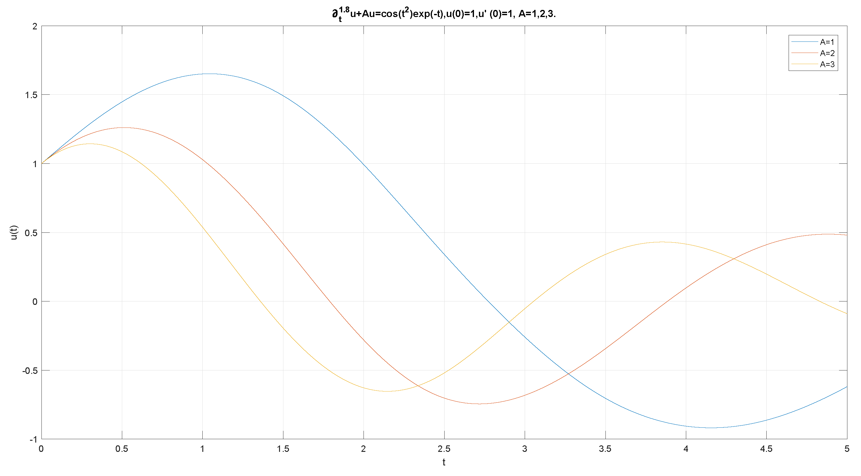
By choosing the function $cos(t^2)exp(-t),$ we get the following relaxations oscillation equation with fractional order given by

$$\begin{array}{c}\hfill {\partial }_t^{1.8}u(t)+Au(t)=cos(t^2)exp(-t),u(0)=1,u^{\prime }(0)=1,\end{array}$$

(33)

where A is the operator mentioned above.

The graphical illustration of Example 2 is depicted in the Figure 1.

7. Discussion

This paper presents a fractional sub-diffusion equation of an impulsive system (3) and its dual (19). The unique continuation Property 2 of the dual system plays a crucial role in the proof of our main result, approximate controllability Theorem 3 of the primal system with an interior control acts on a sub-domain. As an example, the approximate controllability of a fractional relaxation-oscillation equation is discussed and simulated for different relaxation coefficients.

References

- Metzler, R.; Klafter, J. The random walk’s guide to anomalous diffusion: A fractional dynamics approach. Phys. Rep. 2000, 339, 1–77. [Google Scholar] [CrossRef]
- Abada, N.; Benchohra, M.; Hammouche, H. Existence and controllability results for nondensely defined impulsive semilinear functional differential inclusions. J. Differ. Equ. 2009, 246, 3834–3863. [Google Scholar] [CrossRef]
- Chu, J.; Nieto, J.J. Impulsive periodic solutions of first-order singular differential equations. Bull. Lond. Math. Soc. 2009, 40, 143–150. [Google Scholar] [CrossRef]
- Fan, Z.; Li, G. Existence results for semilinear differential equations with nonlocal and impulsive conditions. J. Funct. Anal. 2010, 258, 1709–1727. [Google Scholar] [CrossRef]
- Bainov, D.; Simeonov, P. Impulsive Differential Equations: Periodic Solutions and Applications; CRC Press: Boca Raton, FL, USA, 1993; Volume 66. [Google Scholar]
- Sun, J.; Chen, H.; Nieto, J.J. Infinitely many solutions for second-order Hamiltonian system with impulsive effects. Math. Comput. Model. 2011, 54, 544–555. [Google Scholar] [CrossRef]
- Lions, J.L. Optimal Control of Systems Governed Partial Differential Equations; Springer: New York, NY, USA, 1971. [Google Scholar]
- Bergounioux, M.; Penalization, A. Method for Optimal Control of Elliptic Problems with State Constraints. SIAM J. Control Optim. 1992, 30, 305–323. [Google Scholar] [CrossRef]
- Debbouche, A.; Torres, D.F.M. Approximate Controllability of Fractional Nonlocal Delay Semilinear Systems in Hilbert Spaces. Int. J. Control 2013, 86, 1577–1585. [Google Scholar] [CrossRef]
- Debbouche, A.; Torres, D.F.M. Approximate Controllability of Fractional Delay Dynamic Inclusions with Nonlocal Control Conditions. Appl. Math. Comput. 2014, 243, 161–175. [Google Scholar] [CrossRef]
- Khalida, A.; Benchohra, M.; Meghnafi, M. Controllability for impulsive fractional evolution equations with state-dependent delay. Mem. Differ. Equ. Math. Phys. 2018, 73, 1–20. [Google Scholar]
- Mahto, L.; Abbas, S. Approximate controllability and existence of optimal control of impulsive fractional semilinear functional differential equations with non-local condition. J. Abstr. Differ. Equ. Appl. 2013, 4, 44–59. [Google Scholar]
- Mahmudov, N.I. Partial-approximate controllability of nonlocal fractional evolution equations via approximating method. Appl. Math. Comput. 2018, 334, 227–238. [Google Scholar] [CrossRef]
- Fujishiro, K.; Yamamoto, M. Approximate controllability for fractional diffusion equations by interior control. Appl. Anal. 2014, 93, 1793–1810. [Google Scholar] [CrossRef]
- Love, E.R.; Young, M.L.C. On fractional integration by parts. Proc. Lond. Math. Soc. 1937. [Google Scholar] [CrossRef]
- Sakamoto, K.; Yamamoto, M. Initial value/boundary value problems for fractional diffusion-wave equations and applications to some inverse problems. J. Math. Anal. Appl. 2011, 382, 426–447. [Google Scholar] [CrossRef]
- Samko, S.G.; Kilbas, A.A.; Marichev, O.I. Fractional Integrals and Derivatives; Gordon and Breach Science Publishers: Philadelphia, PA, USA, 1993. [Google Scholar]
- Nigmatulin, R. The realization of the generalized transfer equation in a medium with fractal geometry. Phys. Status Solidi B 1986, 133, 425–430. [Google Scholar] [CrossRef]
- Adams, R.A. Sobolev Spaces; Academic Press: New York, NY, USA, 1975. [Google Scholar]
- Podlubny, I. Fractional Differential Equations; Academic Press: San Diego, CA, USA, 1999. [Google Scholar]
- Russell, D.L. Controllability and stabilizability theory for linear partial differential equations: Recent progress and open questions. SIAM Rev. 1978, 20, 639–739. [Google Scholar] [CrossRef]
- Micu, S.; Zuazua, E. An Introduction to the Controllability of Partial Differential Equations, Quelques Questions de Théorie du Contrôle. In Collection Travaux en Cour; Sari, T., Ed.; 2004; pp. 69–157. Available online: https://cel.archives-ouvertes.fr/cel-00392196/document (accessed on 7 January 2019).
- Protter, M.H. Unique Continuation for Elliptic Equations. Trans. Am. Math. Soc. 1960, 95, 81–90. [Google Scholar] [CrossRef]
- Kilbas, A.A.; Srivastava, H.M.; Trujillo, J.J. Theory and Applications of Fractional Differential Equations; North-Holland Mathematical Studies; Elsevier (North-Holland) Science Publishers: Amsterdam, The Netherlands; London, UK; New York, NY, USA, 2006; Volume 204. [Google Scholar]
Figure 1.
Comparison of solution of (33) with varied relaxation coefficients, and
© 2019 by the authors. Licensee MDPI, Basel, Switzerland. This article is an open access article distributed under the terms and conditions of the Creative Commons Attribution (CC BY) license (http://creativecommons.org/licenses/by/4.0/).
Share and Cite
MDPI and ACS Style
Mahto, L.; Abbas, S.; Hafayed, M.; Srivastava, H.M. Approximate Controllability of Sub-Diffusion Equation with Impulsive Condition. Mathematics 2019, 7, 190. https://0-doi-org.brum.beds.ac.uk/10.3390/math7020190
AMA Style
Mahto L, Abbas S, Hafayed M, Srivastava HM. Approximate Controllability of Sub-Diffusion Equation with Impulsive Condition. Mathematics. 2019; 7(2):190. https://0-doi-org.brum.beds.ac.uk/10.3390/math7020190
Chicago/Turabian StyleMahto, Lakshman, Syed Abbas, Mokhtar Hafayed, and Hari M. Srivastava. 2019. "Approximate Controllability of Sub-Diffusion Equation with Impulsive Condition" Mathematics 7, no. 2: 190. https://0-doi-org.brum.beds.ac.uk/10.3390/math7020190
Note that from the first issue of 2016, this journal uses article numbers instead of page numbers. See further details here.