Subordination Approach to Space-Time Fractional Diffusion

Institute of Mathematics and Informatics, Bulgarian Academy of Sciences, Acad. G. Bonchev str., Bld. 8, Sofia 1113, Bulgaria
*
Author to whom correspondence should be addressed.
Mathematics 2019, 7(5), 415; https://0-doi-org.brum.beds.ac.uk/10.3390/math7050415
Submission received: 30 March 2019
/
Revised: 27 April 2019
/
Accepted: 2 May 2019
/
Published: 9 May 2019
(This article belongs to the Special Issue Advanced Mathematical Methods: Theory and Applications)
Abstract
:The fundamental solution to the multi-dimensional space-time fractional diffusion equation is studied by applying the subordination principle, which provides a relation to the classical Gaussian function. Integral representations in terms of Mittag-Leffler functions are derived for the fundamental solution and the subordination kernel. The obtained integral representations are used for numerical evaluation of the fundamental solution for different values of the parameters.
Keywords:
space-time fractional diffusion equation; fractional Laplacian; subordination principle; Mittag-Leffler function; Bessel functionMSC:
26A33; 33E12; 35R11; 47D061. Introduction
This work is concerned with the n-dimensional space-time fractional diffusion equation
where , is the Caputo time-fractional derivative [1,2]
and , , is the full-space fractional Laplace operator in . Ten equivalent definitions of the fractional Laplacian are given in the survey paper [3]. In particular, it can be defined as a pseudo-differential operator, as follows:
where denotes the Fourier transform of a function f at the point . In the one-dimensional case is the Riesz space-fractional derivative of order .
The space-time fractional diffusion Equation (1) has been extensively studied [4,5,6,7,8,9,10,11,12,13,14,15]. The solution of Problem (1) is given in terms of the fundamental solution and the initial function , as follows:
Therefore, the behavior of the solution to Problem (1) is determined by the properties of the fundamental solution. In this paper, we limit our attention to representations of the fundamental solution .
In the classical case , Equation (1) reduces to the standard diffusion equation with the fundamental solution , given by the Gaussian function (see e.g., [16]):
In the fractional-order setting, the following closed-form representations for the fundamental solution are known:
where denotes the Mittag-Leffler function (see (18)), is the exponential integral [17]
and U is the Tricomi’s confluent hypergeometric function [17]
Representation (4) can be found in a more general setting in [5]. Formula (5) was first derived in the paper [10]. Formula (6) is established in the early work [4]. A derivation of representations (4)–(7) using the subordination relation (see (10)) can be found in [15]. In [13,15], additional closed-form representations for the fundamental solution were derived from (4)–(6) by applying the relations between and . However, all such simple closed-form expressions for the fundamental solution in terms of known special functions are limited to particular values of the parameters.
Extensive research has been devoted to representations of the fundamental solution in the form of the Mellin-Barnes integral or the Fox H-function, such as in [5,6,11] for the one-dimensional and [12,13,14] for the multi-dimensional space-time fractional diffusion-wave equation. One of the advantages of such representations is that the asymptotic behavior of the fundamental solution can be derived from them, because the asymptotic behavior of the Fox H-function has been well-studied (see e.g., [18] or [19]).
An alternative approach to dealing with the space-time fractional diffusion Equation (1) is based on the subordination formula, which relates the fundamental solution and the Gaussian function as follows [14,15]
where is a unilateral probability density function (pdf) in , that is:
The subordination kernel depends on the similarity variable and admits the representation [14]
where the function can be defined as the inverse Laplace transform of the Mittag-Leffler function , that is:
It is worth noting that some known basic properties of follow in a straightforward way from the subordination relation (10), taking into account that the subordination kernel is a pdf. In this way, we can prove that for any dimension , the fundamental solution is a spatial pdf evolving in time:
Therefore, , , inherits this property of the classical Gaussian kernel . In a similar way, estimates for the fundamental solution can be derived from known estimates for the Gaussian kernel . For example, since (see e.g., [16], Remark 3.7.10.), the subordination Formula (10), together with properties (11) imply
A principle of subordination is closely related to the concept of subordination in stochastic processes [20,21]. It has been extensively studied and employed in the context of fractional order equations. The subordination principle for space-fractional evolution equations has been established in [22] in the setting of abstract Cauchy problems. Subordination formulae for the one-dimensional space-time fractional diffusion equation have been studied in [6,9]. In [14,15], subordination principles for the multi-dimensional space-time fractional diffusion equation are deduced. In the case of time-fractional evolution equations with general time-fractional operators, subordination principles have been studied and employed in [23,24,25,26,27,28].
Based on the subordination principles for space- and time-fractional diffusion equations and the dominated convergence theorem, exact asymptotic expressions for the fundamental solution of the multi-dimensional space-time fractional diffusion equation and more general nonlocal equations have recently been established in [29]. For completeness, we next present the asymptotic expansions for , , from [29], Corollary 2.6 (written in our notations and in a slightly more compact form):
If , then
If , then
The asymptotic expansions (14) and (15) are in agreement with those obtained for particular ranges of parameter values in, for example, [5,11,15], as well as with the asymptotic behavior of the closed-form solutions (4)–(7), which can be checked by taking into account the asymptotic expansions for the exponential integral ([17], Eqs. 5.1.11 and 5.1.51)
and for the Tricomi’s confluent hypergeometric function ([17], Section 13.5)
and using some basic properties of the Gamma function.
In the present work, the subordination Formula (10) serves as a starting point for deriving integral representations for the fundamental solution . First, an integral representation for the subordination kernel is established in terms of the Mittag-Leffler function of complex argument. Let us note that a study of the function is of interest, since it also plays the role of subordination kernel related to problems with more general spatial operators, such as in [15]. In addition, coincides with the solution of the one-dimensional space-time fractional diffusion equation with the Riesz-Feller space-fractional derivative of order and skewness , as well as the Caputo time-derivative of order , studied in [5] (see [15], Remark 3). Next, based on the subordination Formula (10), we derive integral representations for the fundamental solution in terms of Mittag-Leffler functions, which are appropriate for numerical implementation.
The paper is organized as follows. Definitions and basic properties of Mittag-Leffler functions and Bessel functions of the first kind are listed in the next section. In Section 3, an integral representation for the subordination kernel is established. In Section 4, computable integral representations for the fundamental solution are derived for and used for numerical experiments.
2. Preliminaries
For and , the following asymptotic expansion for large holds true in the sector of the complex plane
Therefore, taking into account the identity for we derive from (19) two useful asymptotic expressions for and
The faster decay for large of the second function in (20), compared to the first, will be used essentially in this work.
The relations
can be derived directly from the definition (18) of the Mittag-Leffler function; (21) and (20) imply that, by differentiation of the Mittag-Leffler function , a faster decay for large can be achieved.
We point out the following representation of the Mittag-Leffler functions as Laplace transforms (see [31]):
where , , excluding the case . Expression (22) is appropriate for numerical computation of the Mittag-Leffler functions. Let us note, however, that (22) is valid only for real values of . For computation of the Mittag-Leffler function of complex arguments, another technique should be used (see e.g., [32]).
The Bessel function of the first kind is defined by the series [17]
The following particular expressions are of interest in the present work:
The asymptotic expansions of the Bessel function for small and large real arguments are as follows:
3. An Integral Representation for the Subordination Kernel
Representations of the subordination kernel are useful in view of the integral expression (10) for the fundamental solution. In a limited number of particular cases, the subordination kernel can be expressed in terms of elementary functions [15,16,22]:
However, for arbitrary values of the fractional parameters, explicit expressions are not available and other types of representations are needed.
The following Laplace transform pairs for the subordination kernel can be derived from (12) and (13) (see also [15]):
and
In this section, we deduce an integral representation of the subordination kernel by inversion of the Laplace transform pair (29). We choose (29) instead of (28), because of the faster decay for large arguments of the correponding Mittag-Leffler function (see (20)).
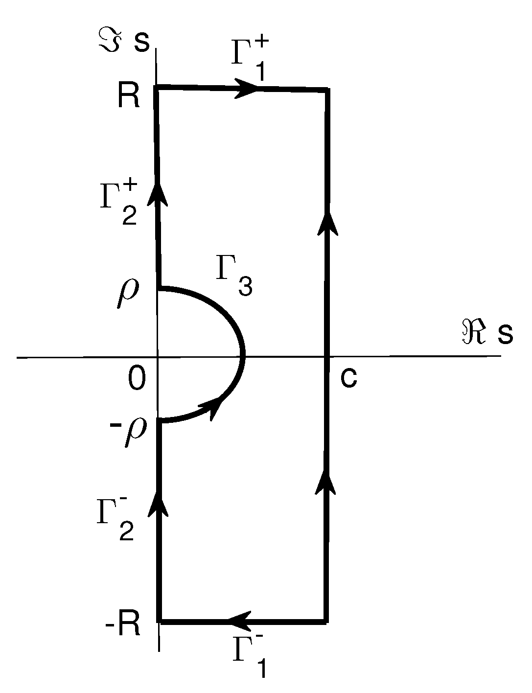
Assume and . Applying the complex Laplace inversion formula to (29) yields:
where means the principal branch of the corresponding multi-valued function defined in the whole complex plane cut along the negative real semi-axis. Since the Mittag-Leffler function is an entire function, is analytic for . Therefore, by the Cauchy’s theorem, the integral in (30) can be replaced by an integral over the composite contour , where
with an appropriate orientation (see Figure 1) and letting , .
Since as , for the integration on as we obtain
due to the asymptotic expansion (20) for the Mittag-Leffler function, which is satisfied since . The integral on is treated in the same way.
Concerning the integral over , we have
since the Mittag-Leffler function under the integral sign is bounded as . Therefore, (30)–(32) imply that is given by the integral over along the imaginary axis with and . This implies:
Therefore,
We observe that the integral in (33) is convergent, since the integrand behaves as for and as for due to the asymptotic Expansion (20) for the Mittag-Leffler function. The representation (33) can also be rewriten in the form
where
For the numerical implementation of Formula (34), the real and imaginary parts above can be numerically calculated by employing a method of computation of the Mittag-Leffler function of complex arguments.
In the particular case of (time-fractional diffusion), representation (34) yields the following simpler formula for the subordination kernel
4. Integral Representations for the Fundamental Solution
According to the subordination Relation (10) and the formula for the Gaussian kernel (3), the fundamental solution of Problem (1) admits the representation
Subordination Formula (36) yields after the change of variables
Applying the formula for the Laplace transform ([35], Section 4.1, Eq. (25))
where denotes the Bessel Function (23) and , we deduce from (37) and (28) the following representation:
The obtained integral representation (38) is not new—see, for example, [12,13,14], where it is deduced by applying a different argument.
Let us first note that for , the integral in (38) is always convergent and gives the following representation for the fundamental solution to the space-fractional diffusion equation:
We observe, however, that if , the integral in (38) is convergent only for very limited ranges for the values of the other two parameters. Indeed, according to the asymptotic expansions of the Bessel and the Mittag-Leffler functions, (25) and (20), the integral in (38) is convergent only in the following cases: and or and . If , the integral is divergent for any . Our aim here is to derive from (38) convergent integral representations for , which hold for all .
First, let . Plugging in (38), the representation for from (24) yields:
which, according to (20), is convergent at only if , unless . However, we can improve the convergence by performing integration by parts in (39). We use the identity
which is derived from (21). In this way, the following integral representation is established:
The asymptotic Expression (20) indicates that the integral in (41) is convergent for all . In the particular case , representation (41) can also be found in [15], Equation 4.13.
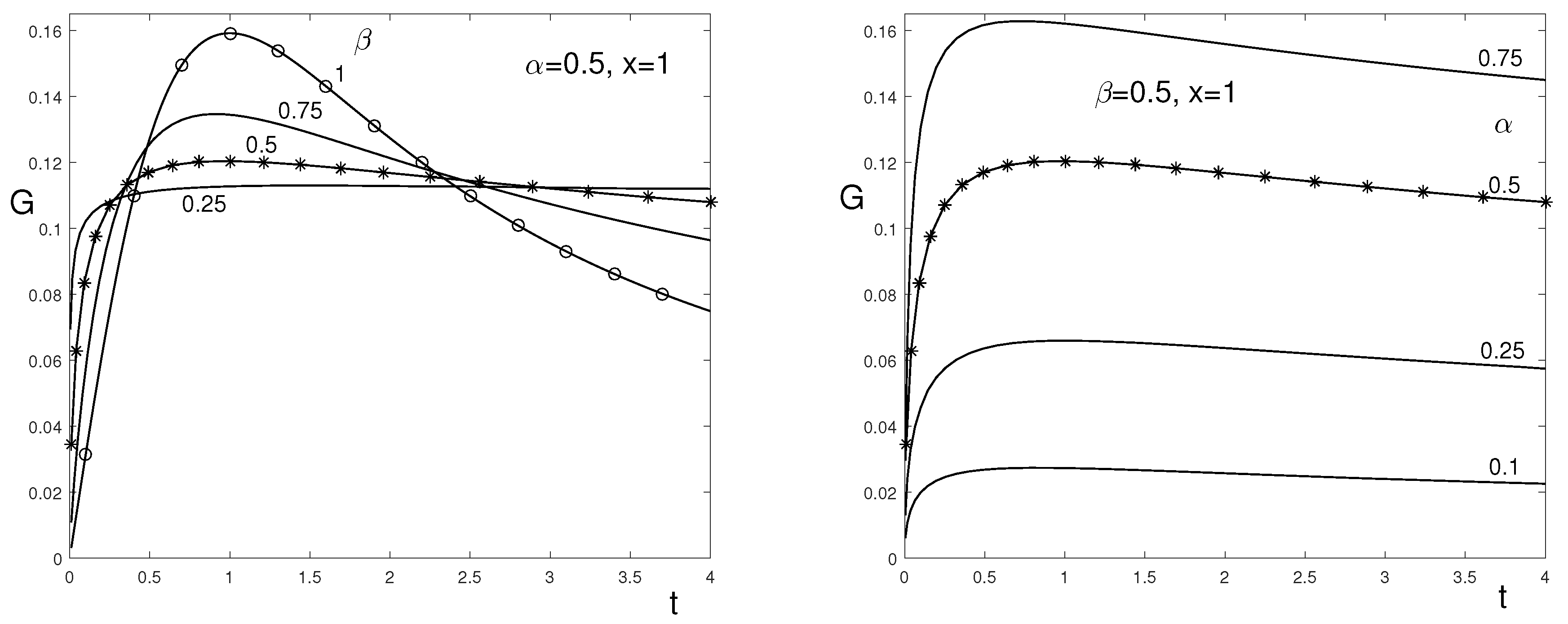
Representation (41) was used for the numerical evaluation of the one-dimensional fundamental solution, and the results are given in Figure 3. For numerical computation of the Mittag-Leffler function in (41), the integral representation (22) was used. Figure 3 shows that the numerical results based on Formula (41) are in good agreement with the exact solutions, (4) and (6).
Next, let us consider . Plugging in the general Formula (38), the representation for from (24) yields:
This integral is divergent for all . Integration by parts gives
and, by applying Formula (40), we obtain the following integral expression for the three-dimensional fundamental solution
where
The asymptotic Expansions (20) of the Mittag-Leffler functions imply that the integral in (42) is convergent for and . Again applying integration by parts in (42) yields
where and therefore, by (43) and (21),
The asymptotic behavior of the Mittag-Leffler functions (20) implies that the integral in (44) is convergent for all .
In an analogous way, for , we deduce from (38) and (24)
where the function is defined in (45). The integral in (46) is convergent for all .
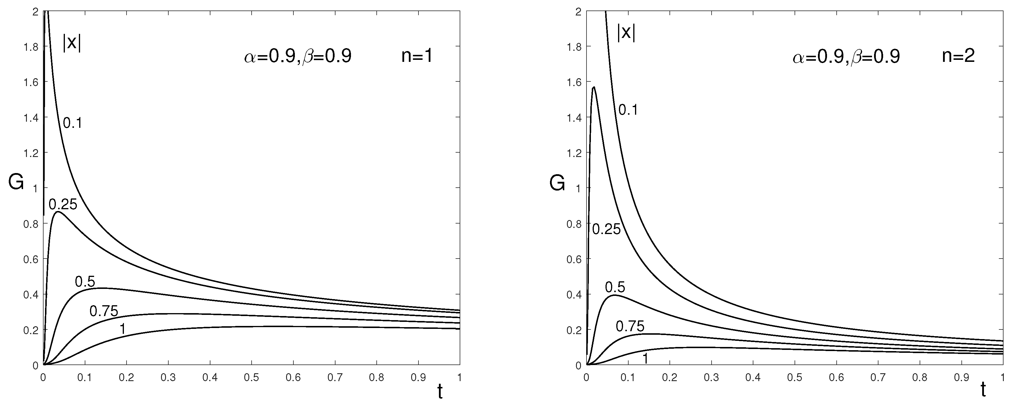
It is verified numerically that integral representations (41), (46) and (44) for the two- and three-dimensional fundamental solutions are in agreement with the exact Solutions (5) and (7). For the numerical computation of the Mittag-Leffler functions in , the integral representation (22) is used.
Numerical results and comparison of the one- and two-dimensional fundamental solutions are given in Figure 4.
For a discussion on other integral representations for the fundamental solution, we refer to [7,12].
All numerical computations in this work were performed with the help of MATLAB.
5. Concluding Remarks
The subordination principle for space-time fractional diffusion equations is a useful tool for finding integral representations of the fundamental solution. The derived integral representations (41), (46) and (44) for , respectively, are appropriate for numerical implementation. The performed numerical experiments confirm that the analytical findings in this work are in agreement with the known exact solutions.
The technique used in the present work for deriving the integral representation for the subordination kernel does not rely on the scaling property and can be extended to equations with more general nonlocal operators in space, such as those considered in [36], as well as operators with a general memory kernel in time, as in [24,37].
Author Contributions
Analytical results and writing, E.B.; numerical implementation and visualization, I.B.
Funding
The first author (E.B.) is partially supported by the National Scientific Program “Information and Communication Technologies for a Single Digital Market in Science, Education and Security (ICTinSES)”, contract No DO1–205/23.11.2018, financed by the Ministry of Education and Science in Bulgaria. The second author (I.B.) is partially supported by Bulgarian National Science Fund (Grant K-06-H22/2).
Acknowledgments
The authors are grateful to the referees for careful reading of the paper and valuable suggestions and comments.
Conflicts of Interest
The authors declare no conflict of interest.
References
- Podlubny, I. Fractional Differential Equations; Academic Press: San Diego, CA, USA, 1999. [Google Scholar]
- Kilbas, A.A.; Srivastava, H.M.; Trujillo, J.J. Theory and Applications of Fractional Differential Equations; North-Holland Mathematics Studies; Elsevier: Amsterdam, The Netherlands, 2006. [Google Scholar]
- Kwaśnicki, M. Ten equivalent definitions of the fractional Laplace operator. Fract. Calc. Appl. Anal. 2017, 20, 7–51. [Google Scholar] [CrossRef]
- Saichev, A.; Zaslavsky, G. Fractional kinetic equations: Solutions and applications. Chaos 1997, 7, 753–764. [Google Scholar] [CrossRef]
- Mainardi, F.; Luchko, Y.; Pagnini, G. The fundamental solution of the space-time fractional diffusion equation. Fract. Calc. Appl. Anal. 2001, 4, 153–192. [Google Scholar]
- Mainardi, F.; Pagnini, G.; Gorenflo, R. Mellin transform and subordination laws in fractional diffusion processes. Fract. Calc. Appl. Anal. 2003, 6, 441–459. [Google Scholar]
- Hanyga, A. Multi-dimensional solutions of space-time-fractional diffusion equations. Proc. R. Soc. Lond. A 2002, 458, 429–450. [Google Scholar] [CrossRef]
- Meerschaert, M.M.; Sikorski, A. Stochastic Models for Fractional Calculus; De Gruyter Studies in Math; Walter de Gruyter: Berlin, Germany; Boston, MA, USA, 2012; Volume 43. [Google Scholar]
- Gorenflo, R.; Mainardi, F. Subordination pathways to fractional diffusion. Eur. Phys. J. Spec. Top. 2011, 193, 119–132. [Google Scholar] [CrossRef] [Green Version]
- Luchko, Y. A new fractional calculus model for the two-dimensional anomalous diffusion and its analysis. Math. Model. Nat. Phenom. 2016, 11, 1–17. [Google Scholar] [CrossRef]
- Luchko, Y. Entropy production rate of a one-dimensional alpha-fractional diffusion process. Axioms 2016, 5, 6. [Google Scholar] [CrossRef]
- Luchko, Y. On some new properties of the fundamental solution to the multi-dimensional space- and time-fractional diffusion-wave equation. Mathematics 2017, 5, 76. [Google Scholar] [CrossRef]
- Boyadjiev, L.; Luchko, Y. Mellin integral transform approach to analyze the multidimensional diffusion-wave equations. Chaos Solit. Fract. 2017, 102, 127–134. [Google Scholar] [CrossRef]
- Luchko, Y. Subordination principles for the multi-dimensional space-time-fractional diffusion-wave equation. Theory Probab. Math. Stat. 2018, 98, 121–141. [Google Scholar]
- Bazhlekova, E. Subordination principle for space-time fractional evolution equations and some applications. Integr. Transf. Spec. Funct. 2019, 30, 431–452. [Google Scholar] [CrossRef]
- Arendt, W.; Batty, C.J.K.; Hieber, M.; Neubrander, F. Vector-Valued Laplace Transforms and Cauchy Problems; Birkhäuser: Basel, Switzerland, 2011. [Google Scholar]
- Abramowitz, M.; Stegun, I. Handbook of Mathematical Functions with Formulas, Graphs, and Mathematical Tables; Dover: New York, NY, USA, 1964. [Google Scholar]
- Braaksma, B.L.J. Asymptotic expansions and analytic continuations for a class of Barnes-integrals. Compos. Math. 1963, 15, 239–341. [Google Scholar]
- Kilbas, A.A.; Saigo, M. H-Transforms: Theory and Applications; Chapman & Hall/CRC Press: Boca Raton, FL, USA, 2004. [Google Scholar]
- Feller, W. An Introduction to Probability Theory and Its Applications; Willey: New York, NY, USA, 1971; Volume 2. [Google Scholar]
- Schilling, R.; Song, R.; Vondraček, Z. Bernstein Functions: Theory and Applications; De Gruyter: Berlin, Germany, 2010. [Google Scholar]
- Yosida, K. Functional Analysis; Springer: Berlin, Germany, 1965. [Google Scholar]
- Kochubei, A.N. Distributed order calculus and equations of ultraslow diffusion. J. Math. Anal. Appl. 2008, 340, 252–281. [Google Scholar] [CrossRef] [Green Version]
- Kochubei, A.; Kondratiev, Y.; da Silva, J.L. Random time change and related evolution equations. arXiv 2019, arXiv:1901.10015. [Google Scholar]
- Bazhlekova, E. Subordination principle for a class of fractional order differential equations. Mathematics 2015, 3, 412–427. [Google Scholar] [CrossRef]
- Bazhlekova, E.; Bazhlekov, I. Subordination approach to multi-term time-fractional diffusion-wave equation. J. Comput. Appl. Math. 2018, 339, 179–192. [Google Scholar] [CrossRef]
- Bazhlekova, E. Subordination in a class of generalized time-fractional diffusion-wave equations. Fract. Calc. Appl. Anal. 2018, 21, 869–900. [Google Scholar]
- Sandev, T.; Tomovski, Ž.; Dubbeldam, J.; Chechkin, A. Generalized diffusion-wave equation with memory kernel. J. Phys. A Math. Theor. 2019, 52, 015201. [Google Scholar] [CrossRef]
- Deng, C.-S.; Schilling, R.L. Exact asymptotic formulas for the heat kernels of space and time-fractional equations. arXiv 2019, arXiv:1803.11435v2. [Google Scholar]
- Gorenflo, R.; Kilbas, A.A.; Mainardi, F.; Rogosin, S.V. Mittag-Leffler Functions: Related Topics and Applications; Springer: Berlin, Germany, 2014. [Google Scholar]
- Gorenflo, R.; Mainardi, F. Fractional calculus: Integral and differential equations of fractional order. In Fractals and Fractional Calculus in Continuum Mechanics; Carpinteri, A., Mainardi, F., Eds.; Springer: Wien, Austria; New York, NY, USA, 1997; pp. 223–276. [Google Scholar]
- Gorenflo, R.; Loutchko, J.; Luchko, Y. Computation of the MittagLeffler function and its derivatives. Fract. Calc. Appl. Anal. 2002, 5, 491–518. [Google Scholar]
- Paneva-Konovska, J. From Bessel to Multi-Index Mittag-Leffler Functions: Enumerable Families, Series in Them and Convergence; World Sci. Publ.: London, UK, 2016. [Google Scholar]
- Paneva-Konovska, J. Differential and integral relations in the class of multi-index Mittag-Leffler functions. Fract. Calc. Appl. Anal. 2018, 21, 254–265. [Google Scholar] [CrossRef]
- Erdelyi, A.; Magnus, W.; Oberhettinger, F.; Tricomi, F.G. Tables of Integral Transforms; McGraw-Hill: New York, NY, USA, 1954; Volume 1. [Google Scholar]
- Biswas, A.; Lörinczi, J. Maximum principles for the time-fractional Cauchy problems with spatially non-local components. Fract. Calc. Appl. Anal. 2018, 21, 1335–1359. [Google Scholar] [CrossRef]
- Tomovski, Ž.; Sandev, T.; Metzler, R.; Dubbeldam, J. Generalized space–time fractional diffusion equation with composite fractional time derivative. Physica A 2012, 391, 2527–2542. [Google Scholar] [CrossRef]
Figure 1.
Contour .

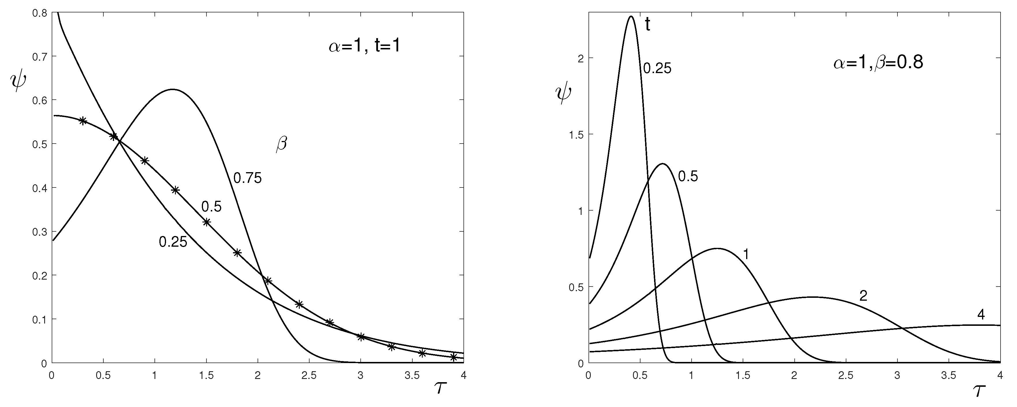
Figure 2.
Subordination kernel as a function of for: and different values of (left); and different values of t (right). Numerical computations are based on Equation (35). The exact Expression (26) for is given by symbols (*).

Figure 3.
The fundamental solution as a function of t for: , and different values of (left); , and different values of (right). Numerical computations are based on Formula (41). Exact Solution (6) for is given by symbols (*); exact solution for computed using (4) is given by symbols ().

Figure 4.
The fundamental solution for and as a function of t for and different values of . One-dimensional solution (left) and two-dimensional solution (right).
Figure 4.
The fundamental solution for and as a function of t for and different values of . One-dimensional solution (left) and two-dimensional solution (right).

© 2019 by the authors. Licensee MDPI, Basel, Switzerland. This article is an open access article distributed under the terms and conditions of the Creative Commons Attribution (CC BY) license (http://creativecommons.org/licenses/by/4.0/).
Share and Cite
MDPI and ACS Style
Bazhlekova, E.; Bazhlekov, I. Subordination Approach to Space-Time Fractional Diffusion. Mathematics 2019, 7, 415. https://0-doi-org.brum.beds.ac.uk/10.3390/math7050415
AMA Style
Bazhlekova E, Bazhlekov I. Subordination Approach to Space-Time Fractional Diffusion. Mathematics. 2019; 7(5):415. https://0-doi-org.brum.beds.ac.uk/10.3390/math7050415
Chicago/Turabian StyleBazhlekova, Emilia, and Ivan Bazhlekov. 2019. "Subordination Approach to Space-Time Fractional Diffusion" Mathematics 7, no. 5: 415. https://0-doi-org.brum.beds.ac.uk/10.3390/math7050415
Note that from the first issue of 2016, this journal uses article numbers instead of page numbers. See further details here.