An Introduction to Space–Time Exterior Calculus


Department of Information and Communication Technologies, Universitat Pompeu Fabra, 08018 Barcelona, Spain
*
Author to whom correspondence should be addressed.
Mathematics 2019, 7(6), 564; https://0-doi-org.brum.beds.ac.uk/10.3390/math7060564
Submission received: 21 May 2019
/
Revised: 17 June 2019
/
Accepted: 18 June 2019
/
Published: 21 June 2019
(This article belongs to the Special Issue Advanced Mathematical Methods: Theory and Applications)
Abstract
:The basic concepts of exterior calculus for space–time multivectors are presented: Interior and exterior products, interior and exterior derivatives, oriented integrals over hypersurfaces, circulation and flux of multivector fields. Two Stokes theorems relating the exterior and interior derivatives with circulation and flux, respectively, are derived. As an application, it is shown how the exterior-calculus space–time formulation of the electromagnetic Maxwell equations and Lorentz force recovers the standard vector-calculus formulations, in both differential and integral forms.
1. Introduction
Vector calculus has, since its introduction by J. W. Gibbs [1] and Heaviside, been the tool of choice to represent many physical phenomena. In mechanics, hydrodynamics and electromagnetism, quantities such as forces, velocities and currents are modeled as vector fields in space, while flux, circulation, divergence or curl describe operations on the vector fields themselves.
With relativity theory, it was observed that space and time are not independent but just coordinates in space–time [2] (pp. 111–120). Tensors like the Faraday tensor in electromagnetism were quickly adopted as a natural representation of fields in space–time [3] (pp. 135–144). In parallel, mathematicians such as Cartan generalized the fundamental theorems of vector calculus, i.e., Gauss, Green, and Stokes, by means of differential forms [4]. Later on, differential forms were used in Hamiltonian mechanics, e.g., to calculate trajectories as vector field integrals [5] (pp. 194–198).
A third extension of vector calculus is given by geometric and Clifford algebras [6], where vectors are replaced by multivectors and operations such as the cross and the dot products subsumed in the geometric product. However, the absence of an explicit formula for the geometric product hinders its widespread use. An alternative would have been the exterior algebra developed by Grassmann which nevertheless has received little attention in the literature [7]. An early work in this direction was Sommerfeld’s presentation of electromagnetism in terms of six-vectors [8].
We present a generalization of vector calculus to exterior algebra and calculus. The basic notions of space–time exterior algebra, introduced in Section 2, are extended to exterior calculus in Section 3 and applied to rederive the equations of electromagnetism in Section 4. In contrast to geometric algebra, our interior and exterior products admit explicit formulations, thereby merging the simplicity and intuitiveness of standard vector calculus with the power of tensors and differential forms.
2. Exterior Algebra
Vector calculus is constructed around the vector space , where every point is represented by three spatial coordinates. In relativity theory the underlying vector space is and time is treated as a coordinate in the same footing as the three spatial dimensions. We build our theory in space–time with k time dimensions and n space dimensions. The number of space–time dimensions is thus and we may refer to a - or -space–time, . We adopt the convention that the first k indices, i.e., , correspond to time components and the indices represent space components and both k and n are non-negative integers. A point or position in this space–time is denoted by , with components in the canonical basis , that is
Given two arbitrary canonical basis vectors and , then their dot product in space–time is
For convenience, we define the symbol as the metric diagonal tensor in Minkowski space–time [2] (pp. 118–120), such that time unit vectors have negative norm , whereas space unit vectors have positive norm . The dot product of two vectors and is the extension by linearity of the product in Equation (2), namely
2.1. Grade, Multivectors, and Exterior Product
In addition to the -dimensional vector space with canonical basis vectors , there exist other natural vector spaces indexed by ordered lists of m non-identical space and time indices for every . As there are such lists, the dimension of this vector space is . We shall refer to m as grade and to these vectors as multivectors or grade-m vectors if we wish to be more specific. A general multivector can be written as
where the summation extends to all possible ordered lists with m indices. If , the list is empty and the corresponding vector space is . The direct sum of these vector spaces for all m is a larger vector space of dimension , the exterior algebra. In tensor algebra, multivectors correspond to antisymmetric tensors of rank m. In this paper, we study vector fields , namely multivector-valued functions varying over the space–time position .
The basis vectors for any grade m may be constructed from the canonical basis vectors by means of the exterior product (also known as wedge product), an operation denoted by ∧ [9] (p. 2). We identify the vector for the ordered list with the exterior product of :
In general, we may compute the exterior product as follows. Let two basis vectors and have grades and , where and are the lengths of the respective index lists. Let denote the concatenation of I and J, let denote the signature of the permutation sorting the elements of this concatenated list of indices, and let denote the resulting sorted list, which we also denote by . Then, the exterior product of is defined as
The exterior product of vectors and is the bilinear extension of the product in Equation (6),
Since permutations with repeated indices have zero signature, the exterior product is zero if or more generally if both vectors have at least one index in common. Therefore, the exterior product is either zero or a vector of grade . Further, the exterior product is a skew-commutative operation, as we can also write Equation (6) as .
At this point, we define the dot product · for arbitrary grade-m basis vectors and as
where I and J are the ordered lists and . As before, we extend this operation to arbitrary grade-m vectors by linearity.
Finally, we define the complement of a multivector. For a unit vector with grade m, its Grassmann or Hodge complement [10] (pp. 361–364), denoted by , is the unit -vector
where is the complement of the list I, namely the ordered sequence of indices not included in I. As before, is the signature of the permutation sorting the elements of the concatenated list containing all space–time indices. In other words is the basis vector of grade whose indices are in the complement of I. In addition, we define the inverse complement transformation as
We extend the complement and its inverse to general vectors in the space–time algebra by linearity.
2.2. Interior Products
While the exterior product of two multivectors is an operation that outputs a multivector whose grade is the addition of the input grades, the dot product takes two multivectors of identical grade and subtracts their grades, yielding a zero-grade multivector, i.e., a scalar. We say that the exterior product raises the grade while the dot product lowers the grade. In this section, we define the left and right interior products of two multivectors as operations that lower the grade and output a multivector whose grade is the difference of the input multivector grades.
As always, we start by defining the operation for the canonical basis vectors. Let and be two basis vectors of respective grades and . The left interior product, denoted by ⨼, is defined as
If I is not a subset of J, that is when there are elements in I not present in J, e.g., for , the signature of the permutation sorting the concatenated list is zero as there are repeated indices in the list to be sorted, and the left interior product is zero. Otherwise, if I is a subset of J, the permutation rearranges the indices in J in such a way that the last positions coincide with I and represents the first elements in the rearranged sequence, that is .
The right interior product, denoted by ⨽, of two basis vectors and is defined as
As with the left interior product, if J is a subset of I, then the permutation rearranges the indices in I so that the first positions coincide with J, otherwise the right interior product is zero.
In general, we have that , as verified in Appendix A.1. We note that these interior products are not commutative, unless either or is an even number, e.g., when , in which case both interior products coincide with the dot product of the two vectors. The interior products may therefore be seen as generalizations of the dot product.
As with the dot and the exterior products, the value of the interior products does not depend on the choice of basis and we may thus compute the left interior product of two vectors and as
and a similar expression holds for the right interior product . Both are grade-lowering operations, as the left (resp. right) interior product is either zero or a multivector of grade (resp. ).
The interior products are not independent operations from the exterior product, as they can be expressed in terms of the latter, the Hodge complement and its inverse (proved in Appendix A.2):
If and are 1-vectors and is an r-vector, then we have the following expression
as proved in Appendix A.3. This expression can be seen as a generalization of the vectorial expression
in the vector space , i.e., a , space–time. This fact is built of the realization that the cross product between two vectors and can be expressed in the following alternative ways
Whenever it holds that , the interior and exterior products are related by the following:
Having introduced the basic notions of space–time exterior algebra, the next section focuses on operations with elements in the exterior algebra, namely integrals and derivatives of vector fields.
3. Integrals and Derivatives of Vector Fields: Circulation and Flux
3.1. Oriented Integrals
Integrals are, together with derivatives, the fundamental mathematical objects of calculus. For example, operations on vectors fields lying in exterior algebra such as the flux and the circulation are expressed in terms of integrals over high-dimensional geometric objects. The integral of an m-graded vector field over a hypersurface of the same dimension, denoted as
is the limit of the Riemann sums for the dot product over points in the hypersurface, where is an m-dimensional infinitesimal vector element. For any , the infinitesimal vector element is given by the sum of all possible differentials for ℓ-dimensional hypersurfaces in a space–time, and is represented in the canonical basis as
where for a given list each differential is given by .
As in traditional calculus, the integral in Equation (21) exhibits coordinate invariance, while the integrand is regarded as an oriented object. Orientation is well defined for integrals along a curve from one point to another, or integrals over a surface oriented at the direction of the normal to the surface. Switching the extreme points of the curve, or taking the opposite direction of the normal would induce a change of sign in the line and surface integrals. In our generalization of vector calculus, a positive orientation is implicit in the ordering of the canonical basis. The skew-symmetry property of the exterior product Equation (6) may introduce sign changes to compensate an eventual change of orientation after changes of coordinates such as permutations of the space–time components.
For a given hypersurface , a convenient transformation for solving the integral in Equation (21) is one such that, at a given point in the hypersurface, the infinitesimal vector element has one component that is tangent to the hypersurface at that point. Let be a unit m-graded vector parallel to at point , and let form an orthonormal basis of such that for the given point in . This change of coordinates from the canonical basis to the new basis is described by a unitary matrix U, dependent on , and that satisfies
Being a unitary matrix, the determinant of U is . Assuming an orientation-preserving change of coordinates, that is , the infinitesimal vector element in Equation (22) for can be expressed as
where is the set of indices for the unit vectors in the new basis orthogonal to . Since all elements in the summation in Equation (24) have at least one differential element lying outside the integration hypersurface, their integrals vanish and therefore
In analogy to , a multivector of grade m, we define a unit -grade vector normal to at point such that . From Equation (10), we see that one such normal multivector with the correct orientation is
For the common spaces considered in vector calculus, and , and according to Equation (23), orientation-preserving changes of coordinates must respectively satisfy and , where is the basis element normal to . These two equalities turn out to describe the counterclockwise (resp. right-hand rule) orientation when conventionally points outside an integration path for (resp. a surface for ) [5] (pp. 184–185).
Building on the concepts and operations of circulation and flux in vector calculus, the right and left interior products lead to general definitions of circulation and flux of multivector fields in exterior algebra along and across hypersurfaces of arbitrary number of dimensions.
3.2. Circulation and Flux of Multivector Fields
Definition 1.
The circulation of a vector fieldof grade m along an ℓ-dimensional hypersurface, denoted by, is given by
Expressing the vector field in the canonical basis and using the definition of in Equation (22), the circulation can be specified in some cases of interest. For , the circulation reads
For instance, for and , this formula recovers the definition the circulation of a vector field along a closed path with the appropriate orientation.
Alternatively, using Equation (25), we note that is integrated along the direction of , tangential to the hypersurface, in an orientation-preserving change of coordinates, that is
Intuitively, the circulation Equation (27) measures the alignment of an m-vector field with respect to for any ℓ and m, with the circulation being an -vector if and zero otherwise.
Definition 2.
The flux of a vector fieldof grade m across an ℓ-dimensional hypersurface, denoted by, is given by
Expressing both and in the canonical basis, and using the inverse Hodge operation in Equation (10), the flux in the special case of can be written as
As an example in , the flux of a vector field through a surface reads
The right-hand side of Equation (32) is a conventional surface integral, upon the identification of as an infinitesimal surface element .
Alternatively, using the analogous of Equation (25) for the differential vector element , the equivalent to Equation (29) for the flux is
This equation implies that is integrated along a normal component to the hypersurface since is a multivector of grade orthogonal to . Intuitively, the flux Equation (30) measures the magnitude of the multivector field crossing the hypersurface. In general, the flux is a vector of grade if and zero otherwise. For instance, if , the flux of over an -dimensional hypersurface gives the integral of over , an extension of the volume integral to ,
where we used the relation , implying that , and that .
3.3. Exterior and Interior Derivatives
In vector calculus, extensive use is made of the nabla operator ∇, a vector operator that takes partial space derivatives. For instance, operations such as gradient, divergence or curl are expressed in terms of this operator. In our case, we need the generalization to space–time to the differential vector operator , defined as , that is
For a given vector field of grade m, we define the exterior derivative of as , namely
The grade of the exterior derivative of is , unless , in which case the exterior derivative is zero, as can be deduced from the fact that all signatures are zero.
In addition, we define the interior derivative of as , namely
The grade of the interior derivative of is , unless , in which case the interior derivative is zero, as implied by the fact that the grade of is larger than the grade of . Using Equation (16) with and assuming that and are 1-vectors, we obtain a generalization of Leibniz’s product rule
The formulas for the exterior and interior derivatives allow us express some common expressions in vector calculus. For a scalar function , its gradient is given by its exterior derivative , while for a vector field , its divergence is given by its interior derivative . From Equation (16) we further observe that for a scalar function we recover the relation
In addition, for a vector fields in , taking into account Equation (18) then the curl can be variously expressed as
This formula allows us to write the curl of a vector field in terms of the exterior and interior products and the Hodge complement, while generalizing both the cross product and the curl to grade-m vector fields in space–time algebras with different dimensions. Moreover, from Equation (16) we can recover for the well-known formula for the curl of the curl of a vector,
It is easy to verify that the exterior derivative of an exterior derivative is zero, as is the interior derivative of an interior derivative, that is for any vector field , we have that
In regard to the vector space , and using Equation (18), these expressions imply the well-known facts that the curl of the gradient and the divergence of the curl are zero:
3.4. Stokes Theorem for the Circulation
In vector calculus in , the Kelvin-Stokes theorem for the circulation of a vector field of grade 1 along the boundary of a bidimensional surface relates its value to that of the surface integral of the curl of the vector field over the surface itself. In the notation used in the previous section, the surface integral is the flux of the curl of the vector field across the surface and this theorem reads
Taking into account the identity in Equation (40), we rewrite the right-hand side in Equation (46) as
where we used that for vectors , . The flux of the curl of the vector field across a surface is also the circulation of the exterior derivative of the vector field along that surface.
The generalized Stokes theorem for differential forms [4] (p. 80) allows us to extend the Kelvin-Stokes theorem to multivectors of any grade m as we do in the following theorem.
Theorem 1.
The circulation of a grade-m vector fieldalong the boundaryof an ℓ-dimensional hypersurfaceis equal to the circulation of the exterior derivative ofalong:
As hinted at above, the role of the vector curl in the right-hand side of Equation (46) is played by the exterior derivative in this generalized theorem.
Proof.
We start by stating the generalized Stokes Theorem for differential forms [4] (p. 80)
where is a differential form and its exterior derivative, represented by the operator
Expressing the circulations in Equation (48) by means of the integrals in Equation (27), we obtain
In the integral in the left-hand side of Equation (51), the integrand is a differential form . After expanding the interior product using the definitions of and we obtain
Then, computing the exterior derivative of this form with Equation (50) gives
We next write down the integrand in the right-hand side of Equation (51), , that is
and verify that it coincides with exterior derivative in Equation (53). As the set of m indices is included in the sets or in Equation (53) or (54), we may write for some . Then, we obtain the following chain of equalities for the basis elements in Equations (53) and (54):
Therefore, and using that , we can write Equation (54) as
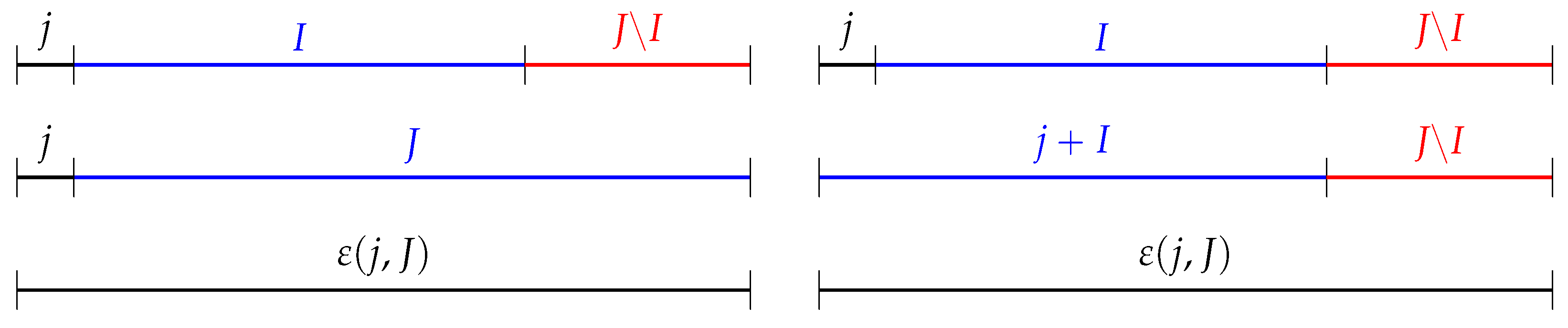
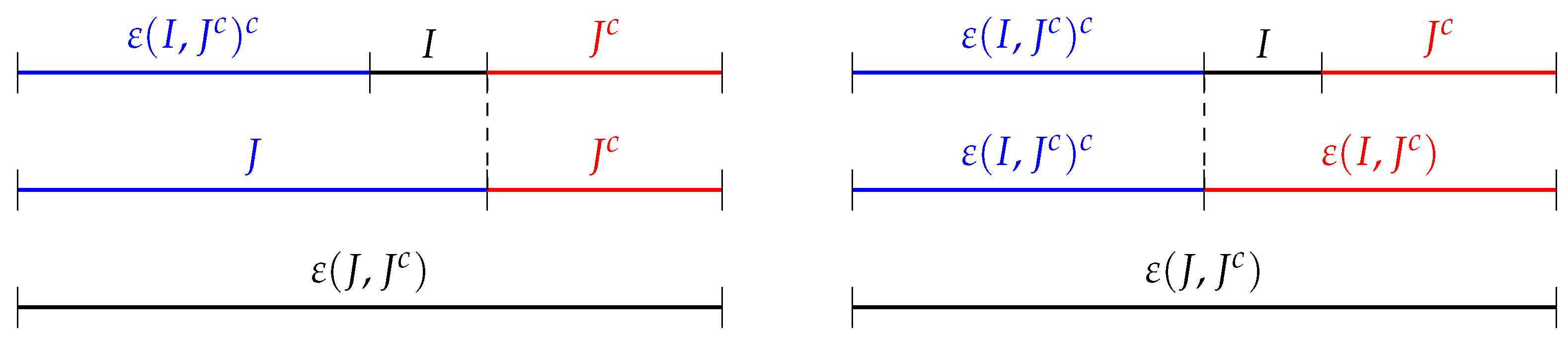
To prove Equation (57) we exploit that the are permutation signatures and that the signature of the composition of permutations is the product of the respective signatures. We proceed with the help of a visual aid in Figure 1, which depicts the identity between two different ways of sorting the concatenated list . On the left column we first sort the list to obtain J and then sort the list . On the right column, we first sort the list and then the list . This proves Equation (57) and the theorem.
Finally, we note that, had we defined the circulation with the left interior product, we would have got an incompatible relation in Equation (57), which could not be solved. □
3.5. Stokes Theorem for the Flux
In vector calculus in , the Gauss theorem relates the volume integral of the divergence of a vector field over a region to the surface integral of the vector field over the region boundary . In the notation used in previous sections, and taking into account that both the surface integral and the volume integral can be expressed as fluxes for , this theorem reads
Making use of the identity , we can rewrite the right-hand side in Equation (58) as
In other words, the Gauss theorem relates the flux of the interior derivative of a vector field across a region to the flux of the vector field itself across the region boundary .
The generalized Stokes theorem for differential forms allows us to extend the Gauss theorem to multivectors of any grade m as we do in the following theorem.
Theorem 2.
The flux of a grade-m vector fieldacross the boundaryof an ℓ-dimensional hypersurfaceis equal to the flux of the interior derivative ofacross:
Proof.
As in the proof of Theorem 1, we apply the Stokes theorem for differential forms in Equation (49) upon the identifications with and with . First, for , we get
Now, taking the exterior derivative of Equation (62), we obtain
This quantity should be equal to in the right-hand side of Equation (61), which we expand as
We first consider the sets in the summations in the alternative expressions for , Equations (63) and (64). Since contains j and is a subset of I, but does not contain j and is also a subset of I (with ), then we can assert that so that the conditions in the summations are equivalent. The basis elements coincide and so do the differentials and derivatives, and it remains to verify the identity
With the definition , and expressed in terms of j, J, and L, this condition gives
Multiplying both sides of the equation by , and , and taking into account that the square of a signature is , we obtain
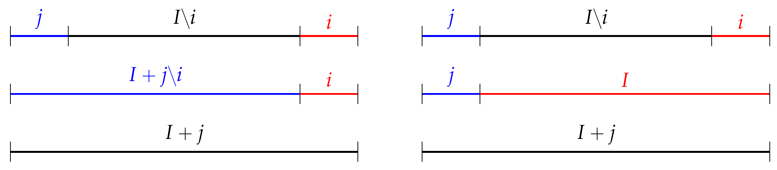
We start by simplifying Equation (67) by noting that
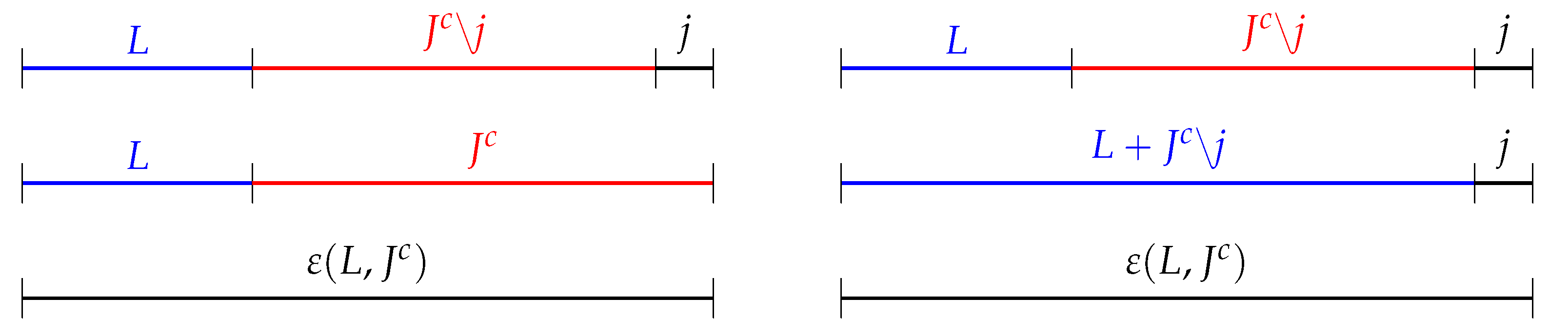
with help of the visual aid in Figure 2. The permutations on the left column first merge with j and then the resulting with L. Similarly, on the right column, we start with L, and , then concatenate and then add j, getting the same result as the left column.
4. An Application to Electromagnetism in 1 + 3 Dimensions
In this section, we show how to recover the standard form of Maxwell equations and Lorentz force in dimensions from a formulation with exterior calculus involving an electromagnetic bivector field and a 4-dimensional current density vector . In the appropriate units, the bivector field can be decomposed as , where contains the electric-field time-space components and contains the space-space components for the magnetic field . Similarly, the current density depends on the charge density and the spatial current density . More specifically,
Here the Hodge complement acts only on the space components, and . The bivector field is closely related to the Faraday tensor, a rank-2 antisymmetric tensor.
Maxwell equations, in their differential form, constrain the divergence of the electric and the magnetic field, Equations (72) and (73), respectively, and the curl of and , namely Equations (74) and (75) [11] (p. 4-1).
We refer to Equations (73) and (74) as homogeneous Maxwell equations and to Equations (72) and (75) as inhomogeneous Maxwell equations, as they include the fields and the sources given by charge and current densities. In exterior-calculus notation, both pairs of equations can be combined into simple multivector equations,
where is the differential operator for and . As a consistency check, note that the wedge product raises the grade of , and the zero in Equation (76) is the zero trivector; also, as the left interior product lowers the grade of , both sides of Equation (77) relate space–time vectors.
Next to Maxwell equations, the Lorentz force density characterizes, after integrating over the appropriate region, the force exerted by the electromagnetic field upon a system of charges described by the charge and current densities and [11] (pp. 13-1–13-3),
In relativistic form, the Lorentz force density becomes a four-dimensional vector [2] (pp. 153–157). The time component of this vector is , the power dissipated per unit of volume, or after integrating over the appropriate region, the rate of work being done on the charges by the fields. In exterior-calculus notation, the Lorentz force density vector can be computed as a left interior product, namely
4.1. Equivalence of the Lorentz Force Density
In this section, we prove that Equation (79) indeed recovers the relativistic Lorentz force density by verifying that its components in both vector-calculus and exterior-calculus coincide. From the definitions of and , and using the distributive property of the interior product, we get
Some straightforward calculations give , , and . In addition, the formula for the left interior product in Equation (18) gives , where the cross product is only valid for three dimensions. With these calculations, we obtain
namely, a time-component and a spatial component equal to the Lorentz force density .
4.2. Equivalence of the Differential Form of Maxwell Equations
In this section, we prove that Equation (76) indeed recovers the homogeneous Maxwell equations and that Equation (77) recovers the inhomogeneous Maxwell equations.
First, we observe that the exterior derivative gives a trivector with 4 components, while the homogeneous Maxwell equations are a scalar, Equation (73), and a vector, Equation (74). We shall verify that the scalar equation turns out to be given by the trivector component of , while the vector equation is given by the trivector components , , and of the exterior derivative.
We evaluate the exterior derivative using the decomposition of in Equation (71),
where we used that and that in the second step of Equation (82). Taking advantage of Equation (40) we have the equality , while , and
Indeed, the first summand vanishes when or, taking the inverse Hodge complement, when Equation (74) holds. In terms of components, the spatial Hodge complement in this equation transforms a spatial vector into a bivector with components , , and only and this equation recovers the homogeneous Maxwell equation in Equation (74). After taking the exterior product with , we obtain the trivector components , , and . Similarly, the second term vanishes for , recovering Equation (73). In terms of components, the spatial Hodge complement directly transforms a scalar into a trivector with a unique component , recovering the homogeneous Maxwell equation in Equation (73).
We move on to the inhomogeneous Maxwell equations. We compute the interior derivative ,
since . The interior derivative gives a space–time vector with 4 components, while the inhomogeneous Maxwell equations are a scalar, Equation (72), and a spatial vector, Equation (75).
We can verify that the scalar equation turns out to be given by the vector component of , while the spatial vector equation is given by the spatial vector components , , and of . Indeed, if we match this expression with the current density vector , then the time component of gives Equation (72). Selecting the space components of , the differential equation is
which, using the relation can be written as Equation (75).
4.3. Equivalence of the Integral Form of Maxwell Equations
After studying the exterior-calculus differential formulation of Maxwell equations, we recover the standard integral formulation. Applying the Stokes Theorem 1 to Equation (76), we find that the circulation of the bivector field along the boundary of any three-dimensional space–time volume is zero:
At this point, Equation (86) is a scalar equation and we obtain the pair of homogeneous Maxwell equations by considering two different hypersurfaces .
First, let the domain contain only spatial coordinates. There are no tangential components to V with time indices and the contribution of to the circulation of over in Equation (86) is zero, i.e.,
Using that for any vectors , , and therefore and the definition , the integral in the right-hand side of Equation (87) becomes
where we used Equation (32) to write the last surface integral. Substituting Equation (88) back into Equation (86) gives the Gauss law for the magnetic field [11] (pp. 1-5–1-9).
Let now be a time-space domain , where S is a two-dimensional spatial surface. With no real loss of generality we assume that S lies on the plane. Its boundary is the union of the sets , and . For the first set, we choose as the vector normal to pointing outwards on the plane defined by S and , where is a vector tangent to with a counterclockwise orientation, so that . Further, since is a time-space bivector, the contribution of to the circulation of over this first set in Equation (86) is zero, and
Writing the differential vector as , parameterizing the line integral over the boundary by the variable x with unit vector , and using that and therefore , the integral of the right-hand side of Equation (89) becomes
For the second and third sets the normal vector to the integration surface pointing outwards are and respectively. Since is a space-space bivector in both cases, then the contribution of to the circulation is zero. We express the circulations of as fluxes of and surface integrals as done in Equation (88). Using these observations the integral for the circulation of over these two sets in Equation (86) is given by
Combining Equations (90) and (91) in Equation (86) we recover the integral over time of the so called Faraday law [11] (pp. 17-1–17-2). Equivalently, taking the time derivative recovers the usual Faraday law, namely
In regard to the inhomogeneous Maxwell equations, applying the Stokes Theorem 2 to Equation (77), we find that the flux of the bivector field across the boundary of any three-dimensional space–time volume is equal to the flux of the current density across the three-dimensional space–time volume:
As with the homogeneous Maxwell equations, the scalar Equation (93) yields the inhomogeneous Maxwell equations by considering two different hypersurfaces .
First, let the integration domain be a spatial volume V. Since there are no normal components to V with space indices only, the contribution of to the flux is zero so that Equation (93) becomes
From the definition of inverse Hodge complement in Equation (10), we write the differential vectors
Plugging these expressions in Equation (94), using the definitions of and , and computing the dot products on both sides of the equality, we obtain that Equation (94) simplifies as
In Equation (98) we used that and in Equation (99) we used that . Since the Hodge complement is over space, the result is a surface integral with positive orientation as in Equation (32). We recovered in Equation (99) the Gauss law for the electric field [11] (pp. 4-7–4-9).
For where S is a two-dimensional surface lying on the plane, the boundary is the union of the sets , and . For the first set, since has no time components, the contribution of to this set is zero, that is
As in the homogeneous case, we choose as the vector normal to pointing outwards on the plane defined by S and , where is a vector tangent to with a counterclockwise orientation, such that introduces a change of sign. Expressing and in the canonical basis, defining so that contains only space indexes, and using that and , we obtain that Equation (100) simplifies to
For the second and third sets we respectively choose and pointing outside , implying that the contribution of is zero for this set as the inverse Hodge complement of is a space vector. Expressing in Equation (95) and using similar steps as in Equations (97)–(99), the left-hand side of Equation (93) over these two sets is given by
Finally, for the right-hand side of Equation (93), we choose as the vector normal to pointing outside. Since implies that , we obtain that
5. Summary
In this paper, we aimed at showing how exterior calculus provides a tool merging the simplicity and intuitiveness of standard vector calculus with the power of tensors and differential forms. Set in the context of a general space–time algebra with multiple space and time components, we provided the basic concepts of exterior algebra and calculus, such as multivectors, wedge product and interior products, with a distinction between left and right products, Hodge complement, and exterior and interior derivatives. While a space–time with multiple time coordinates leads to several issues from the physical point of view [12], we did not deal with these problems as this paper focuses on the mathematical constructions. We also defined oriented integrals, with two important examples being the flux and circulation of grade m-vector fields as integrals of the normal and tangent components of the field to a hypersurface respectively. These operations extend the standard circulation of a vector field as a line integral and the flux of a vector field as a surface integral in three dimensions to any number of dimensions and any vector grade.
Armed with the theory of differential forms, we proved two exterior-calculus Stokes theorems, one for the circulation and one for the flux, that generalize the Kelvin-Stokes, Gauss and Green theorems. We saw that the flux of the curl of a vector field in three dimensions across a surface is also the circulation of the exterior derivative of the vector field along that surface. In exterior calculus, these Stokes theorems hold for any number of dimensions and any vector grade and are simply expressed in terms of the exterior and interior derivatives for the circulation and flux respectively.
As an application of our tools, we showed how to recover the classical laws of electromagnetism, Maxwell equations and Lorentz force, from a exterior-calculus formalism in relativistic space–time with one temporal and three spatial dimensions. The electromagnetic field is described by a bivector field with six components, closely related to Faraday’s antisymmetric tensor, containing both electric and magnetic fields. The differential form of Maxwell equations relates the exterior derivative of the bivector field with the zero trivector and the interior derivative of the field with the current density vector. In the integral form, these equations correspond to the statements that the circulation of the bivector field along the boundary of any three-dimensional space–time volume is zero, and that the flux of the bivector field across the boundary of any three-dimensional space–time volume is equal to the flux of the current density across the same space–time volume.
Author Contributions
Conceptualization, A.M.; Methodology, I.C., J.F.-S., A.M.; Investigation, I.C.; Writing—Original Draft Preparation, I.C.; Writing—Review & Editing, I.C., J.F.-S., A.M.
Acknowledgments
This work has been funded in part by the Spanish Ministry of Economy and Competitiveness under grants TEC2016-78434-C3-1-R and BES-2017-081360.
Conflicts of Interest
The authors declare no conflict of interest.
Appendix A. Proofs of Product Identities
In this appendix, we verify the relations about interior products introduced in Section 2.
Appendix A.1. Relation between Left and Right Interior Products
We now prove the formula
relating left and right interior products. For two lists I and J, we have
where we assumed that with no loss of generality and used that in this case. The only difference between the expressions lies in the signatures, that are related by setting and in the following lemma.
Lemma A1.
Given two arbitrary lists A and B, of lengthandrespectively, then the permutations sorting the concatenated listsandsatisfy the formula
Proof.
Given a list A, let be the reversed list, namely the list where the order of all the elements is reversed. Counting the number of position jumps needed to reverse the list, we obtain the signature of this reversing operation as
The proof is based on the identity between two different ways of rearranging the concatenated list into the ordered list , as depicted in Figure A1.
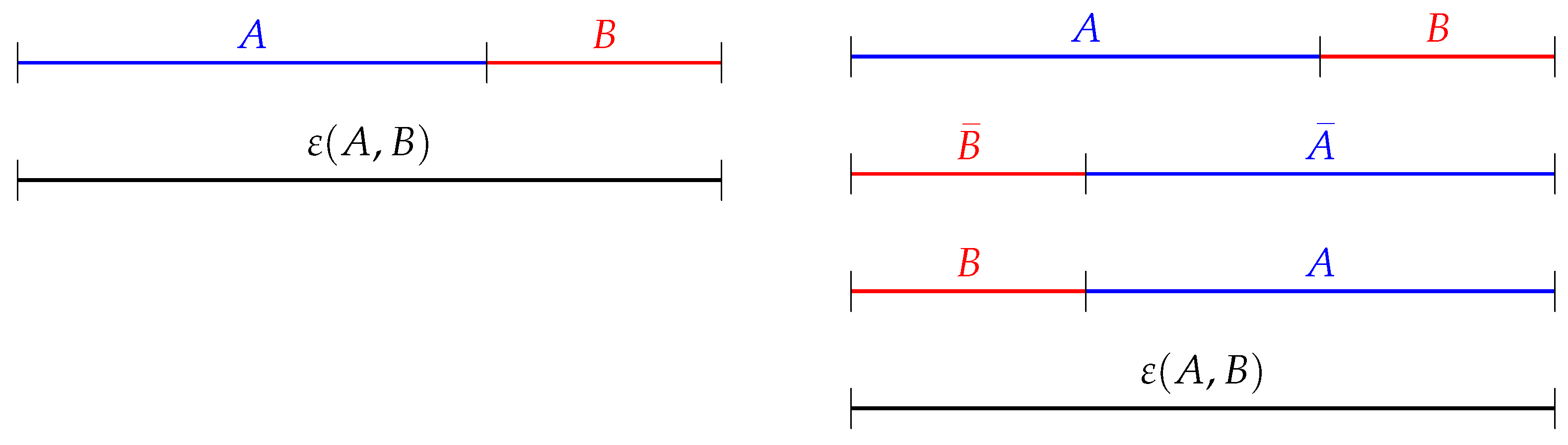
First, in the left column of Figure A1 we depict how a single permutation with signature orders the list . In the right column of Figure A1 we depict how a different series of permutations achieves the same result. We start by reversing the concatenated list , an operation with signature . Then, we separately partially reverse the lists and , operations with respective signatures and . A final permutation with signature orders the list into . Since the signature of a composition of permutations is the product of the signatures, we obtain that
Figure A1.
Visual aid for the relation between and .

Appendix A.2. Relation between Interior and Exterior Products
We start with the expression for the left interior product Equation (14). From Equations (9) and (10), we compute
and since , we can conclude that . If we now compare the result with Equation (11), we need just to verify the identity
or equivalently
The left-hand side of Equation (A9) corresponds to taking the sets , I and , in this order, and then merging and sorting with I and then merging and sorting the resulting set J with , as shown in the left column of Figure A2. On the right-hand side, we start we the same three lists, but we first merge and sort I with , and then we get the whole list by merging and sorting the result with , as represented in the right column of Figure A2. Thus, starting from the three sets and rearranging them in different ways, we get the same final ordered list, and since the signatures of the left-hand side and right-hand side are the same, and Equation (A9) is proved. As a consequence, Equation (14) is verified.
Figure A2.
Visual aid for the permutations in Equation (A9).
Figure A2.
Visual aid for the permutations in Equation (A9).

Afterwards, we prove the formula for the right interior product Equation (15). Using Equations (9) and (10), we write
Using that , in order to prove the validity of Equation (15), we need to prove the relation
We can prove it applying Lemma A1 to obtain the expression Equation (A8), or by following the same procedure as before, paying attention to the difference that now list J is included in I.
Appendix A.3. Triple mixed product
Given two 1-vectors and and a r-vector , we prove the relation
Proof.
We start by evaluating explicitly, separating terms and , namely
then, using and adding and removing a term , we get
More concretely, the left-hand side is given by
Similarly, we evaluate the right-hand side as
Comparing Equations (A15) and (A16), it remains to prove the equality, and now we prove the equality
We rewrite Equation (A17) multiplying both sides for so that we obtain
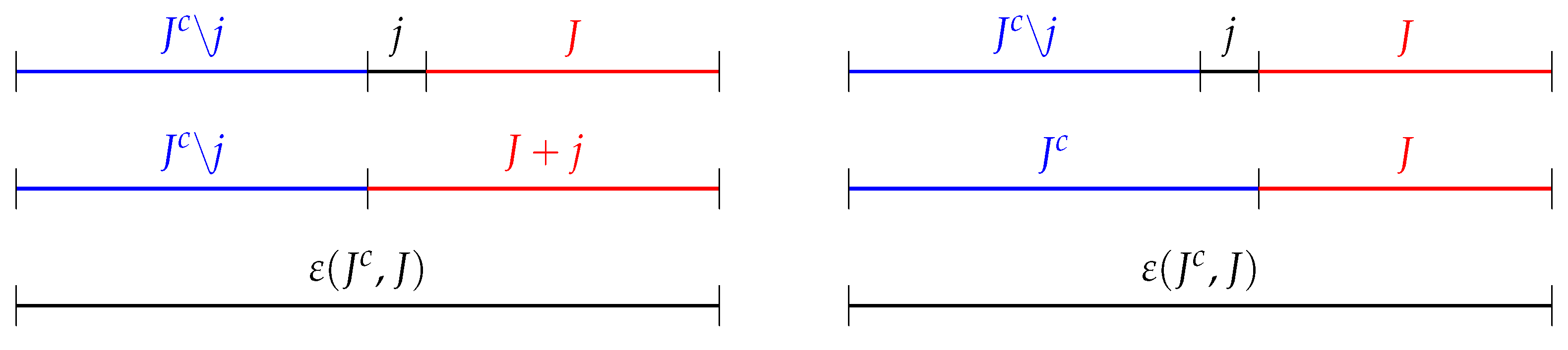
which we verify with the help of Figure A3. On the left column, we first merge j with and then the resulting list with i. On the right columns, the permutations first join and i and the resulting I is then merged with j, getting the same result in both sides of the relation.
Thus, we can write
where we identify the term , and finally conclude
which proves our initial formula. □
Figure A3.
Visual aid for the identity .

References
- Gibbs, J.W.; Wilson, E.B. Vector Analysis; Yale University Press: New Haven, CT, USA, 1929. [Google Scholar]
- Lorentz, H.A.; Einstein, A.; Minkowski, H.; Weyl, H. The Principle of Relativity: A Collection of Original Memoirs on the Special and General Theory of Relativity; Dover Publications: Mineola, NY, USA, 1923. [Google Scholar]
- Ricci, M.M.G.; Levi-Civita, T. Méthodes de calcul différentiel absolu et leurs applications. Math. Ann. 1900, 54, 125–201. [Google Scholar] [CrossRef]
- Cartan, E. Les Systemes Differentiels Exterieurs Et Leurs Applications Geometriques; Hermann & Cie: Paris, France, 1945. [Google Scholar]
- Arnold, V.I.; Weinstein, A.; Vogtmann, K. Mathematical Methods of Classical Mechanics; Springer: Berlin, Germany, 1989. [Google Scholar]
- Clifford, W.K. Mathematical Papers; Macmillan: London, UK, 1882. [Google Scholar]
- Grassmann, H. Extension Theory (History of Mathematics, 19); American Mathematical Society: Providence, RI, USA; London Mathematical Society: London, UK, 2000. [Google Scholar]
- Sommerfeld, A. Zur Relativitätstheorie. I. Vierdimensionale Vektoralgebra. Ann. Phys. 1910, 337, 749–776. [Google Scholar] [CrossRef]
- Winitzki, S. Linear Algebra via Exterior Products; Free Software Foundation: Boston, MA, USA, 2010. [Google Scholar]
- Frankel, T. The Geometry of Physics, 3rd ed.; Cambridge University Press: Cambridge, UK, 2012. [Google Scholar]
- Feynman, R.P.; Leyton, R.B.; Sands, M. The Feynman Lectures on Physics; Addison–Wesley: Boston, MA, USA, 1964; Volume 2. [Google Scholar]
- Velev, M. Relativistic mechanics in multiple time dimensions. Phys. Essays 2012, 25, 403–438. [Google Scholar] [CrossRef] [Green Version]
Figure 1.
Visual aid for the identity among permutations in Equation (57).
Figure 1.
Visual aid for the identity among permutations in Equation (57).

Figure 2.
Visual aid for the identity .

Figure 3.
Visual aid for the identity .

© 2019 by the authors. Licensee MDPI, Basel, Switzerland. This article is an open access article distributed under the terms and conditions of the Creative Commons Attribution (CC BY) license (http://creativecommons.org/licenses/by/4.0/).
Share and Cite
MDPI and ACS Style
Colombaro, I.; Font-Segura, J.; Martinez, A. An Introduction to Space–Time Exterior Calculus. Mathematics 2019, 7, 564. https://0-doi-org.brum.beds.ac.uk/10.3390/math7060564
AMA Style
Colombaro I, Font-Segura J, Martinez A. An Introduction to Space–Time Exterior Calculus. Mathematics. 2019; 7(6):564. https://0-doi-org.brum.beds.ac.uk/10.3390/math7060564
Chicago/Turabian StyleColombaro, Ivano, Josep Font-Segura, and Alfonso Martinez. 2019. "An Introduction to Space–Time Exterior Calculus" Mathematics 7, no. 6: 564. https://0-doi-org.brum.beds.ac.uk/10.3390/math7060564
Note that from the first issue of 2016, this journal uses article numbers instead of page numbers. See further details here.