The Trapezoidal Fuzzy Two-Dimensional Linguistic Power Generalized Hamy Mean Operator and Its Application in Multi-Attribute Decision-Making

School of Economic and Management, Beijing Jiaotong University, Beijing 100044, China
*
Author to whom correspondence should be addressed.
Mathematics 2020, 8(1), 122; https://0-doi-org.brum.beds.ac.uk/10.3390/math8010122
Submission received: 28 October 2019
/
Revised: 25 December 2019
/
Accepted: 8 January 2020
/
Published: 13 January 2020
(This article belongs to the Special Issue Recent Advances in Game and Decision Theory: Structures, Models, Applications and Software Implementation 2019)
Abstract
:As a common information aggregation tool, the Hamy mean (HM) operator can consider the relationships among multiple input elements, but cannot adjust the effect of elements. In this paper, we integrate the idea of generalized a weighted average (GWA) operator into the HM operator, and reduce the influence of related elements by adjusting the value of the parameter. In addition, considering that extreme input data may lead to a deviation in the results, we further combine the power average (PA) operator with HM, and propose the power generalized Hamy mean (PGHM) operator. Then, we extend the PGHM operator to the trapezoidal fuzzy two-dimensional linguistic environment, and propose two new information aggregation tools, the trapezoidal fuzzy two-dimensional linguistic power generalized Hamy mean (TF2DLPGHM) operator and the weighted TF2DLPGHM (WTF2DLPGHM) operator. Some properties and special cases of these operators are discussed. Furthermore, based on the proposed WTF2DLPGHM operator, a new multi-attribute decision-making method is proposed for lean management evaluation of industrial residential projects. Finally, an example is given to show the specific steps, effectiveness, and superiority of the method.
1. Introduction
A classic multi-attribute decision-making (MADM) problem can be described as follows: given a group of possible alternatives in advance, with the help of certain information aggregation tool, evaluate these alternatives from the perspective of multiple attributes. The purpose of decision-making is to find the most satisfactory solution from this group of alternatives. With the progress of human society, the complexity and fuzziness of decision-making environments are also increasing, which makes it difficult to deal with realistic decision-making problems with crisp numbers. In order to solve this problem, Zadeh [1] proposed the fuzzy sets (FSs) theory, which has been widely studied as an effective tool to express fuzzy and uncertain information. Later, many scholars put forward many new extended forms based on the theory to describe uncertain information more accurately, such as triangular fuzzy numbers [2], trapezoidal fuzzy numbers [3], intuitionistic fuzzy sets [4,5], interval-valued intuitionistic fuzzy sets [6,7], type-2 fuzzy sets [8], hesitant fuzzy sets [9], and so on. In view of the convenience of these fuzzy theories for expressing uncertain information, many prospective research results have been obtained [10,11,12,13,14].
All of these fuzzy information forms have a common feature: Decision makers (DMs) can only express their preference information quantitatively with a few crisp numbers. However, because of the hesitation and ambiguity involved in human cognitive thinking, qualitative information representation is easier than quantitative information representation. In 1975, the fuzzy linguistic evaluation method based on linguistic variables was proposed by Zadeh [15], which allows DMs to express preference information qualitatively through single linguistic terms. With the progress in research, more advanced qualitative information representation models, such as uncertain linguistic variables [16], two-dimensional linguistic variables (2DLVs) [17], linguistic intuitionistic fuzzy numbers [18,19], and hesitant fuzzy linguistic term sets [20] have been proposed; they allow DMs to express evaluation information with two or more linguistic terms. In particular, the 2DLVs proposed by Zhu et al. [17] contain two kinds of linguistic information. The evaluation information of the first dimension is the evaluation values of alternatives given by DMs, while the second dimension is used to describe the DMs’ self-judgment for the reliability of the evaluation value. On the whole, two-dimensional linguistic evaluation information covers more complete cognitive preferences, which helps DMs to express their opinions more accurately.
To further improve the accuracy of qualitative linguistic information representation, Liu [21] extended 2DLVs to two-dimensional uncertain linguistic variables (2DULVs), which is one of the most important research results. Since 2DLVs and 2DULVs were put forward, they have been widely studied and have produced many useful research results. Using the MADM method, Liu and Teng [22] extended the TODIM method to a two-dimensional uncertain linguistic environment to deal with MADM problems. Ding and Liu [23] proposed the two-dimensional uncertain linguistic DEMATEL method to determine the critical success factors of emergency management. Zhao et al. [24] extended the PROMETHEE method to a two-dimensional linguistic environment and proposed the possibility degree for 2DLVs. Wu et al. [25] proposed a risk assessment framework of waste-to-energy projects by combining the cloud model and 2DLVs. Using an aggregation operator, Liu et al. [26] extended the GWA operator and hybrid GWA operator to a two-dimensional uncertain linguistic environment to evaluate the decision-making problems in this situation. Considering the possible relationships between elements, Chu and Liu [27] proposed a new weighted generalized Heronian mean operator and weighted generalized geometric Heronian mean operator for 2DULVs. Furthermore, Liu et al. [28] studied an MSM operator in the two-dimensional uncertain linguistic environment and proposed two new MSM operators. In addition, some scholars put forward a new two-dimensional linguistic information form based on 2DLVs. Li et al. [29] proposed trapezoidal fuzzy two-dimensional linguistic variables (TF2DLVs), in which the first dimension is represented by trapezoidal fuzzy numbers, and developed two power generalized aggregation operators based on this information form. Yin et al. [30] further studied a partitioned Bonferroni mean operator in the two-dimensional uncertain linguistic environment to describe the relationships between elements. Liu [31] proposed two-dimensional uncertain linguistic generalized normalized weighted geometric Bonferroni mean.
TF2DLVs are an extended two-dimensional linguistic information form, in which the first dimension is represented by trapezoidal fuzzy numbers, and the second dimension is represented by linguistic terms. Here, the second dimension of linguistic information is used to describe the subjective confidence of DMs for giving the first-dimension evaluation information. Therefore, compared with 2DLVs, TF2DLVs represent a fusion of quantitative and qualitative evaluation information, covering more specific evaluation information, which can effectively avoid the loss of evaluation information. At present, many studies focus on 2DLVs and 2DULVs, while few focus on TF2DLVs. Therefore, this paper will further study TF2DLVs and propose a new MADM method in the trapezoidal fuzzy two-dimensional linguistic environment.
Information aggregation operators that consider the relationships between elements, such as the Heronian mean, Bonferroni mean, Maclaurin symmetric mean, and Hamy mean (HM) [32], have been widely used in various information representation models. However, the Bonferroni mean and Heronian mean can only describe the relationship between two input elements. In some decision-making scenarios, there may be relationships among multiple input elements. As a result, they cannot adapt to this decision-making situation. Instead, the HM operator can flexibly simulate the relationship among multiple input elements. In addition, the power average (PA) [33] operator is another powerful information aggregation tool. The PA operator can eliminate the influence of unreasonable data on the sorting results by giving low weight to extreme data [34,35]. Considering the excellent characteristics of the PA operator and HM operator processing information, recently Liu et al. [36] put forward a power Hamy mean (PHM) operator by combining PA and HM operators. However, HM operator and PHM operator give the same importance to the attributes of interactive operation, so they cannot function like a Bonferroni mean operator, which can enlarge or reduce the influence of attributes by adjusting the parameters.
To make up for this deficiency, this paper integrates the idea of a GWA operator into the HM operator to flexibly adjust the impact of multiple elements. Then, combining it with a PA operator, the power generalized Hamy mean (PGHM) operator is proposed. Furthermore, we extend the PGHM operator to the trapezoidal fuzzy two-dimensional linguistic environment, and propose two new information aggregation tools, the trapezoidal fuzzy two-dimensional linguistic power generalized Hamy mean (TF2DLPGHM) operator and the weighted TF2DLPGHM (WTF2DLPGHM) operator. The proposed operators have three excellent properties. (1) They can integrate the characteristics of the PA operator, which can eliminate the influence of unreasonable data on the sorting results. (2) They can model the relationship among multiple input elements. (3) They can flexibly enlarge or reduce the influence of related elements by adjusting the parameters. Finally, based on the proposed WTF2DLPGHM operator, a new MADM method is proposed to solve the problem of lean management evaluation of industrial residential projects.
The structure of this article is as follows. In Section 2, some related concepts are explained. Section 3 proposes the PGHM operator and extends it to the trapezoidal fuzzy two-dimensional linguistic environment. Then, two new trapezoidal fuzzy two-dimensional linguistic information aggregation operators, i.e., the TF2DLPGHM operator and WTF2DLPGHM, are developed. In Section 4, based on the proposed WTF2DLPGHM operator, we develop a new method for solving MADM problems wherein attribute values are expressed in the form of TF2DLVs. In Section 5, an example is given to demonstrate the effectiveness and superiority of the method. Section 6 gives some conclusions and future research directions.
2. Preliminaries
In this section, we first introduce some basic concepts related to the work done in this paper, such as trapezoidal fuzzy numbers, linguistic term sets, trapezoidal fuzzy two-dimensional linguistic variables, the power average operator, the generalized aggregation operator, and the Hamy mean operator.
2.1. Trapezoidal Fuzzy Numbers
Definition 1
[3]. A trapezoidal fuzzy number (TRFN) can be defined as , and the membership degree function : is defined as follows:
where . The element of is a real number, and its membership function is the regularly and continuous convex function, which indicates the degree to which element belongs to the fuzzy set . In particular, when , the TRFN degenerates into a triangular fuzzy number; when , the TRFN degenerates into a real number.
The distance between and can be expressed as follows:
2.2. Linguistic Term Sets
Suppose is a discrete linguistic term set (LTS) containing an odd number of linguistic terms. Generally speaking, when is 5 or 7, it can be well adapted to the psychological cognition of DMs. In particular, if takes a value of 5, the LTS can be expressed as . For LTS , and should satisfy the following conditions [38]:
- (1)
- The set is ordered: , if and only if ;
- (2)
- There is the negation operator: , such that ;
- (3)
- If , then and .
Considering the loss of information that may occur in the calculation process, Xu [39] further proposed the continuous LTS , which still satisfies the above conditions. Note that is usually used to evaluate alternatives; only appears in the calculation process.
2.3. Trapezoidal Fuzzy Two-Dimensional Linguistic Variables
TF2DLVs are an extended two-dimensional linguistic information form, in which the first dimension is represented by trapezoidal fuzzy numbers, and the second dimension is represented by a linguistic term. Here, the second-dimension linguistic information is used to describe the subjective confidence of DMs for giving the first-dimension evaluation information. Therefore, TF2DLVs cover more specific evaluation information and can effectively avoid the loss of evaluation information.
Definition 2
[29]. Let be a TRFN and be a linguistic term. If is used to express the evaluation value of alternative given by the DM and to indicate the reliability of the evaluation value given by the DM, then a TF2DLV can be obtained.
Let and be any two TF2DLVs and , then the operational rules between and are expressed as follows:
For any three TF2DLVs , and , they have the following relationships:
- (1)
- ;
- (2)
- ;
- (3)
- ;
- (4)
- ;
- (5)
- ;
- (6)
- ;
- (7)
- .
Definition 3
For any two TF2DLVs and , if , then , and vice versa.
Definition 4
2.4. Power Average Operator
Definition 5
represents the support degree from to and satisfies the following properties:
- (1)
- ;
- (2)
- ;
- (3)
- .
2.5. Generalized Aggregation Operator
Definition 6
[40]. Let be a set of nonnegative real numbers, then the GWA operator is expressed as follows:
where is the weighting vector of , and . is a parameter and its range is .
2.6. Hamy Mean Operator
Definition 7
[32]. Let be a set of nonnegative real numbers, then the HM operator is expressed as follows:
where is a parameter of HM operator, and is full combination of . is called the binomial coefficient, where and .
As seen from Definition 7, the greatest advantage of the HM operator is that it can describe the relationship among more than two input elements. In addition, it has the following ideal properties:
- (1)
- If , then ;
- (2)
- If , then ;
- (3)
- If , then ;
- (4)
- .
3. The Trapezoidal Fuzzy Two-Dimensional Linguistic Aggregation Operator
Compared with a Bonferroni mean operator, the HM operator can model the relationship of multiple input elements, but the attributes are given the same importance in the process of describing the attribute interaction. On the contrary, the BM operator can flexibly enlarge or reduce the influence of related elements by adjusting the values of parameters and . Thus, in order to make up for this deficiency, we propose the power generalized Hamy mean (PGHM) operator. The proposed PGHM operator has three functions. One is that by adjusting the value of parameter , the PGHM operator can model the relationship among multiple elements; the other is that by adjusting the value of parameter , the effect of multiple elements can be enlarged or reduced; and the third is that it can eliminate the influence of unreasonable data on sorting results by giving low weight to extreme data. The mathematical expression of the PGHM operator is as follows.
3.1. The Power Generalized Hamy Mean Operator
Definition 8.
Let be a set of nonnegative real numbers and , then the PGHM operator can be expressed as follows:
where is a parameter of the PGHM operator, is a full combination of , and is called the binomial coefficient. Here , in which represents the support degree from to . In addition, it is easy to prove that the PHM operator satisfies the basic properties of the HM operator.
In the following, we introduce a PGHM operator into the trapezoidal fuzzy two-dimensional linguistic environment, and further propose the trapezoidal fuzzy two-dimensional linguistic power generalized Hamy mean (TF2DLPGHM) operator and its weighted form (WTF2DLPGHM).
3.2. The TF2DLPGHM Operator
Definition 9.
Let be a set of TF2DLVs, then the TF2DLPGHM operator can be expressed as follows:
where is a parameter of the TF2DLPGHM operator, is a full combination of , and is called the binomial coefficient. Here , in which represents the support degree from to .
Let , obviously, . The definition of the TF2DLPGHM operator is equivalent to the following form:
Theorem 1.
Let be a group of TF2DLVs, then the expansion of TF2DLPGHM operator is still a TF2DLV, then
The detailed derivation of Equation (23) is shown in Appendix A.
Next, we will discuss some ideal properties of the TF2DLPGHM operator.
Property 1
(Idempotency).Let and be two groups of TF2DLVs. When , we have
Proof.
When , we can get . Then,
Thus, the proof of Property 1 is completed. □
Property 2
(Commutativity).Let and be two groups of TF2DLVs. When is an arbitrary arrangement of , we have
Proof.
When is an arbitrary arrangement of , we can get .
Then, , i.e.,
Thus, the proof of Property 2 is completed. □
Property 3
(Boundedness).Let be a group of TF2DLVs, and , then
Proof.
Since , then .
Therefore, , i.e., .
Thus, the proof of Property 3 is completed. □
Next, we discuss some special cases of the TF2DLPGHM operator when parameters and take different values, as described below.
Case 1. When and , the TF2DLPGHM operator degenerates into the trapezoidal fuzzy two-dimensional linguistic power averaging operator:
Case 2. When , the TF2DLPGHM operator degenerates into the trapezoidal fuzzy two-dimensional linguistic power Hamy mean operator:
Case 3. When and , the TF2DLPGHM operator degenerates into the trapezoidal fuzzy two-dimensional linguistic power geometric average operator:
3.3. The Weighted Form of TF2DLPGHM Operator
Definition 10.
Let be a group of TF2DLVs, be the weighting vector of , and , then the WTF2DLPGHM operator can be expressed as follows:
where is a parameter of the WTF2DLPGHM operator, is a full combination of , and is called the binomial coefficient. Here , in which represents the support degree from to .
Let , obviously . The definition of the WTF2DLPGHM operator is equivalent to the following form:
Theorem 2.
Let be a group of TF2DLVs, then the expansion of WTF2DLPGHM operator is still a TF2DLV, then
The detailed derivation process of Equation (26) is shown in Appendix B.
Example 1.
Let , , and be four TF2DLVs and their subjective weight be ; the WTF2DLPGHM operator is used to aggregate these four elements.
Step 1. Calculate the support degree , where .
Step 2. Calculate the .
Step 3. Calculate the comprehensive weight of each TF2DLV, where .
Step 4. Calculate the comprehensive evaluation value by the WTF2DLPGHM operator (suppose ).
Next, we discuss some special cases of the WTF2DLPGHM operator when parameters and take different values, as described below.
Case 1. When , the WTF2DLPGHM operator degenerates into the operator TF2DLPGHM operator:
Case 2. When and , the WTF2DLPGHM operator degenerates into the weighted trapezoidal fuzzy two-dimensional linguistic power averaging operator:
Case 3. When , the WTF2DLPGHM operator degenerates into the weighted trapezoidal fuzzy two-dimensional linguistic power Hamy mean operator:
Case 4. When and , the TF2DLPGHM operator degenerates into the weighted trapezoidal fuzzy two-dimensional linguistic power geometric average operator:
4. An Approach to MADM with the WTF2DLPGHM Operator
This paper considers a lean management evaluation problem of industrial residential projects based on TF2DLVs. It is assumed that there are alternative projects in lean management evaluation of industrial residential projects. Each alternative has first-class evaluation indicators , whose weight vector is expressed as and satisfies . There are second-class indicators under each first-class indicator . represents the weight vector of each second-class indicator and satisfies . The decision matrix is represented by , where represents the evaluation value of the second-class indicator of the first-class evaluation indicator in alternative . Evaluation values are expressed by TF2DLVs, i.e., , and satisfies ,. Then, we can rank the alternatives according to the given information.
In the following, the proposed WTF2DLPGHM operator is applied to solve such MADM problems. The steps are as follows:
- Step 1.
- Normalize the decision matrix into . For the benefit attribute, we have , and for the cost attribute, we have .
- Step 2.
- Calculate the support degree from the second-class indicator to the second-class indicator of each alternative under the first-class indicator , where .
- Step 3.
- Calculate the .
- Step 4.
- Calculate the comprehensive weight of each second-class indicator under the first-class indicator , where .
- Step 5.
- Calculate the comprehensive evaluation value of each alternative under the first-class indicator by the proposed WTF2DLPGHM operator.
- Step 6.
- Calculate the comprehensive weight of each first-class indicator , where .
- Step 7.
- Calculate the comprehensive evaluation value of each alternative by the proposed WTF2DLPGHM operator.
- Step 8.
- Calculate the expected value of each alternative according to the Definition 3.
- Step 9.
- Sort the alternatives according to the descending order of .
5. A Calculation Example
Example 2.
In order to promote the improvement of industrial lean management level, this paper selects three industrial residential projects to evaluate the implementation level of lean management. Each alternative has five first-class evaluation indicators whose weight vector is expressed as and satisfies . Here, the first-class indicators , , , and have four second-class indicators, which are expressed as , and the first-class indicator have three second-class indicators . In addition, represents the weight vector of the second-class indicators under the first-class indicator and satisfies , and represents the weight vector of the second-class indicators under the first-class indicator and satisfies .
Here, the evaluation index system and index weight of lean management implementation level of industrialized residential projects are shown in Table 1. Based on the evaluation information in the form of TF2DLVs given by DMs, the decision matrix is constructed as shown in Table 2. In particular, DMs use the LTS with five linguistic terms to express the subjective trust in the evaluation results.
5.1. The Decision-Making Steps
Step 1. Because no attribute is a cost type, there is no need to standardize matrix .
Step 2. Calculate the support degree from the second-class indicator to the second-class indicator of each alternative under the first-class indicator . For example, the support degree from to under the first-class indicator is as follows:
Step 3. Calculate the . For example, the about the first-class indicator is as follows:
Step 4. Combining with the subjective weight in Table 1, the comprehensive weight of each second-class indicator under the first-class indicator can be calculated. For example, the weight of each second-class indicator under the first-class indicator is as follows:
Step 5. Calculate the comprehensive evaluation value of each alternative under the first-class indicator by the proposed WTF2DLPGHM operator , and the results are shown in Table 3.
Step 6. Combining with the subjective weight in Table 1, the comprehensive weight of each first-class indicator can be calculated.
Step 7. Calculate the comprehensive evaluation value of each alternative by the proposed WTF2DLPGHM operator .
Step 8. Calculate the expected value of each alternative according to the Definition 3.
Step 9. Sort the alternatives according to the descending order of .
Thus, alternative project has the best level of lean management implementation, and alternative project has the worst level of lean management implementation.
5.2. Parameter Sensitivity Analysis
There are two types of parameters in the proposed WTF2DLPGHM operator, among which is related to the HA operator and k is related to the GWA operator. When the values of and k change, the final ranking results may change. Therefore, in the following, we can observe the ranking results by changing parameters and k. In Table 4, if are all 1, the WTF2DLPGHM operator can reduce into the weighted trapezoidal fuzzy two-dimensional linguistic power Hamy mean (WTF2LPHM) operator; then, by changing the value of , we only analyze the influence of correlation parameter on the calculation results. Table 5 shows the ranking results under different k when two attributes have interrelationships (); Table 6 shows the ranking results under different k when three attributes have interrelationships ().
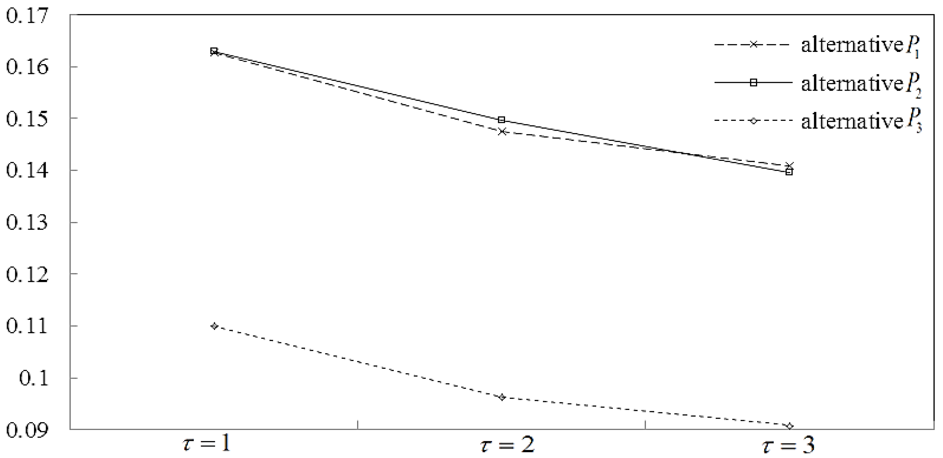
In the following, let be all 1, and discuss the influence of correlation parameter on the calculation results. From Table 4, we can observe that when the parameter is assigned to different values, the ranking results are slightly different. For and , although the values of are different, the ranking orders are exactly the same. For , the alternative is identified as the best alternative, whereas is identified as the second-best alternative for and . This shows that different relationship models will have a certain impact on the ranking results. In addition, from Table 4 and Figure 1, as the value of increases, the expected value of the same alternative decreases. In practice, we can assign different values according to the actual relationship structure among the attributes.
Then, we discuss the influence of parameters on the calculation results. From the data in Table 5, when is less than , the expected values of all alternatives decrease with the increase in , and the ranking results obtained by the proposed WTF2DLPGHM operator are always . On the contrary, when is greater than , the expected values of all alternatives increase with the increase of , the ranking results change significantly, and alternative changes from the second best to the best. Similarly, we can get the same conclusion from Table 6. When is less than and , the expected values of all alternatives decrease with the increase of and , and the ranking results are always . Instead, when is greater than and , the expected values of all alternatives increase with the increase of , and alternative changes from the second best to the best. Combined with the above analysis, we see that the changes in parameters do affect the calculation results. That is to say, by taking different values, the influence degree of input attributes will increase or decrease and the calculated results will change accordingly. Thus, DMs can flexibly adjust the impact of each attribute according to the actual situation.
5.3. Comparative Analysis and Discussion
5.3.1. The Validity of the Proposed Method
In order to prove the validity of the proposed method, we use two existing methods to solve the abovementioned lean management evaluation problem. The first approach is based on the trapezoidal fuzzy two-dimensional linguistic power generalized weighted aggregation (TF2DLPGWA) operator proposed by Li et al. [29], and the second approach is based on the trapezoidal fuzzy two-dimensional linguistic Bonferroni mean (TF2DLBM) operator proposed by Shi [41]. The expected values and ranking results of these different MADM methods are shown in Table 7.
The TF2DLPGWA operator proposed by Li et al. [29] integrates information under the assumption that the attributes are completely independent. For the accuracy of comparison, we set in the proposed WTF2DLPGHM operator, then the WTF2DLPGHM operator degenerates into an operator without considering the attribute relationship. Specially, when and , the proposed WTF2DLPGHM operator can reduce into the weighted trapezoidal fuzzy two-dimensional linguistic power averaging (WTF2DLPA) operator, and the TF2DLPGWA operator proposed by Li et al. [29] also degenerates into WTF2DLPA operator when . As shown in Table 8, under such parameter values, the expected values of the method proposed by Li et al. [29] are exactly the same as in our proposed method. Therefore, when the attributes are completely independent, the consistency of the ranking results of the proposed WTF2DLPGHM operator and the TF2DLPGWA operator [29] greatly proves the effectiveness of the proposed method.
Then, we consider the case of correlation between attributes. The TF2DLBM operator proposed by Shi [41] considers the relationship of two different attributes. In order to discuss the influence of parameter , we first set , and then the proposed WTF2DLPGHM operator becomes an operator similar to the TF2DLBM operator, which only considers the relationship between two attributes. In case of and , the ranking results of the proposed WTF2DLPGHM operator are exactly the same as that of the TF2DLBM operator [41] in the case of . Therefore, the consistency the ranking results of the proposed WTF2DLPGHM operator and the TF2DLBM operator [41] greatly shows the effectiveness of our method.
5.3.2. A Comparison with the TF2DLPGWA Operator
As seen in Table 8, the calculation results of the proposed WTF2DLPGHM operator in the case of and are exactly the same as for the TF2DLPGWA operator [29] in the case of . This is because, under such parameter settings, both the proposed WTF2DLPGHM operator and the TF2DLPGWA operator [29] degenerate into a WTF2DLPA operator without considering attribute correlation. However, for the proposed WTF2DLPGHM operator, when is 2 or 3, the ranking result obtained is completely different to that of the TF2DLPGWA operator [29]. The proposed WTF2DLPGHM operator ( and ) thinks that alternative is better than alternative , and the TF2DLPGWA operator [29] gives the opposite result. The reasons for this are as follows. The TF2DLPGWA operator proposed by Li et al. [29] is based on the simplest PA operator and GWA operator. These operators are developed in a completely independent attributes environment, and have some limitations in terms of practical application. In the lean management evaluation problem of industrial residential projects, there is an obvious relationship between attributes. Therefore, the TF2DLPGWA operator [29] cannot give accurate evaluation results. On the contrary, the proposed WTF2DLPGHM operator combines the excellent characteristics of the Hamy mean operator, and can consider the relationship among multiple input elements flexibly by taking different values for parameter . For example, when is 3, the proposed operator considers the relationship between two attributes, and when is 2, the relationship among three attributes is considered. Therefore, the proposed WTF2DLPGHM operator can adapt to more complex MADM environments.
5.3.3. A Comparison with the TF2DLBM Operator
Compared with the TF2DLBM operator, the proposed WTF2DLPGHM operator has two advantages: one is to integrate the characteristics of the PA operator, which can eliminate the influence of unreasonable data on the sorting results; the other is to model the relationship among multiple input elements by adjusting the parameter (see Table 9 for details).
For the TF2DLBM operator, when , the ranking results are the same as for the proposed WTF2DLPGHM operator when , and , but there is a gap in the ranking results when , , and . The consistency of the former shows the effectiveness of the proposed method and the inconsistency of the latter shows that the parameter has an important impact on the calculation results. The TF2DLBM operator can capture the relationship between two attributes (), and enlarge or reduce the influence degree of corresponding attributes by adjusting the values of and . However, the TF2DLBM operator cannot be handled for a MADM problem in which multiple attributes () have relationships. The proposed WTF2DLPGHM operator can make up for this deficiency. On the one hand, by adjusting the value of , the WTF2DLPGHM operator can model the relationship among multiple attributes; on the other hand, by adjusting the value of , the influence degree of multiple attributes can be enlarged or reduced. Thus, the proposed method has strong flexibility and can deal with complex MADM problems.
6. Conclusions
When describing the relationship between attributes, a traditional Hamy mean operator gives the same importance to the attributes of interactive operation—unlike a Bonferroni mean operator, which can enlarge or reduce the influence of related attributes by adjusting the parameters. In order to make up for this deficiency, we introduce the idea of a generalized weighted average operator into the Hamy mean operator and propose the power generalized Hamy mean (PGHM) operator. Furthermore, we extend the PGHM operator to the trapezoidal fuzzy two-dimensional linguistic environment, and propose two new information aggregation tools, the TF2DLPGHM operator and the WTF2DLPGHM operator. Finally, an example is given to show the specific steps. Compared with the existing two methods, the effectiveness of this method is verified.
Compared with the general MADM methods, the superiority of the proposed method is mainly shown in four aspects: (1) The proposed method takes TF2DLVs as the information representation form, which helps to improve the accuracy of the linguistic information description and reduce the loss of information. (2) The proposed WTF2DLPGHM operator can integrate the characteristics of the PA operator, which can eliminate the influence of unreasonable data on the sorting results. (3) The proposed WTF2DLPGHM operator can model the relationship among multiple input elements. (4) The proposed WTF2DLPGHM operator can enlarge or reduce the influence of related elements by adjusting the parameters. In the future, we will extend the partition HM operator to some new fuzzy information, such as q-Rung Orthopair Fuzzy information [42,43,44,45], the trapezoidal fuzzy two-dimensional linguistic environment to further clarify the interactions between attributes. In the meantime, we can use the proposed method to solve MAGDM problems.
Author Contributions
Conceptualization, Y.L. (Yisheng Liu), Y.L. (Ye Li); Data curation, Y.L. (Yisheng Liu); Formal analysis, Y.L. (Yisheng Liu), Y.L. (Ye Li); Investigation, Y.L. (Ye Li); Methodology, Y.L. (Yisheng Liu), Y.L. (Ye Li); Resources, Y.L. (Yisheng Liu); Software, Y.L. (Ye Li); Supervision, Y.L. (Yisheng Liu); Writing—original draft, Y.L. (Ye Li); Writing—review & editing, Y.L. (Yisheng Liu). All authors have read and agreed to the published version of the manuscript.
Funding
This research received no external funding.
Conflicts of Interest
The authors declare no conflicts of interest.
Appendix A
Proof.
Based on the operational rules of TF2DLVs in Definition 2, we get , .
Then, ,.
Therefore, .
Thus, the proof of Theorem 1 is completed. □
Appendix B
Proof.
Based on the operational rules of TF2DLVs in Definition 2, we can get
Then, ,.
Therefore, .
Thus, the proof of Theorem 2 is completed. □
References
- Zadeh, L.A. Fuzzy sets. Inf. Control 1965, 8, 338–353. [Google Scholar] [CrossRef] [Green Version]
- Yen, K.K.; Ghoshray, S.; Roig, G. A linear regression model using triangular fuzzy number coefficients. Fuzzy Sets Syst. 1999, 106, 167–177. [Google Scholar] [CrossRef]
- Li, R.J. Theory and Application on the Fuzzy Multiple Attribute Decision Making; Science Press: Beijing, China, 2002. [Google Scholar]
- Atanassov, K.T. Intuitionistic fuzzy sets. Fuzzy Sets Syst. 1986, 20, 87–96. [Google Scholar] [CrossRef]
- Liu, P.; Tang, G. Some Intuitionistic Fuzzy Prioritized Interactive Einstein Choquet Operators and Their Application in Decision Making. IEEE ACCESS 2019, 6, 72357–72371. [Google Scholar] [CrossRef]
- Atanassov, K.; Gargov, G. Interval valued intuitionistic fuzzy sets. Fuzzy Sets Syst. 1989, 31, 343–349. [Google Scholar] [CrossRef]
- Liu, P. Some Hamacher aggregation operators based on the interval-valued intuitionistic fuzzy numbers and their application to Group Decision Making. IEEE Trans. Fuzzy Syst. 2014, 22, 83–97. [Google Scholar] [CrossRef]
- Karnik, N.N.; Mendel, J.M. Operations on type-2 fuzzy sets. Fuzzy Sets Syst. 2001, 122, 327–348. [Google Scholar] [CrossRef]
- Torra, V. Hesitant fuzzy sets. Int. J. Intell. Syst. 2010, 25, 529–539. [Google Scholar] [CrossRef]
- Alcantud, J.C.R.; Torra, V. Decomposition theorems and extension principles for hesitant fuzzy sets. Inf. Fusion 2018, 41, 48–56. [Google Scholar] [CrossRef]
- Farhadinia, B.; Herrera-Viedma, E. Multiple criteria group decision making method based on extended hesitant fuzzy sets with unknown weight information. Appl. Soft Comput. 2019, 78, 310–323. [Google Scholar] [CrossRef]
- Ghorabaee, M.K.; Amiri, M.; Zavadskas, E.K.; Turskis, Z.; Antucheviciene, J. A new multi-criteria model based on interval type-2 fuzzy sets and EDAS method for supplier evaluation and order allocation with environmental considerations. Comput. Ind. Eng. 2017, 112, 156–174. [Google Scholar] [CrossRef]
- Nguyen, H. A Generalized p-Norm Knowledge-based Score Function for Interval-valued Intuitionistic Fuzzy Set in Decision Making. IEEE Trans. Fuzzy Syst. 2019, in press. [Google Scholar] [CrossRef]
- Liu, P.; Tang, G.; Liu, W. Induced generalized interval neutrosophic Shapley hybrid operators and their application in multi-attribute decision making. Sci. Iran. 2017, 24, 2164–2181. [Google Scholar] [CrossRef] [Green Version]
- Zadeh, L.A. The concept of a linguistic variable and its application to approximate reasoning-I. Inf. Sci. 1975, 8, 199–249. [Google Scholar] [CrossRef]
- Xu, Z. Induced uncetain linguistic OWA operators applied to group decision making. Inf. Fusion 2006, 7, 231–238. [Google Scholar] [CrossRef]
- Zhu, W.D.; Zhou, G.Z.; Yang, S.L. An approach to group decision making based on 2-dimension linguistic assessment information. Syst. Eng. 2009, 27, 113–118. [Google Scholar]
- Chen, Z.; Liu, P. An approach to multiple attribute group decision making based on linguistic intuitionistic fuzzy numbers. Int. J. Comput. Intell. Syst. 2015, 8, 747–760. [Google Scholar] [CrossRef] [Green Version]
- Liu, P.; Zhang, X. Approach to Multi-Attributes Decision Making with Intuitionistic Linguistic Information based on Dempster-Shafer Evidence Theory. IEEE ACCESS 2018, 6, 52969–52981. [Google Scholar] [CrossRef]
- Rodríguez, R.M.; Martínez, L.; Herrera, F. Hesitant fuzzy linguistic term sets for decision making. IEEE Trans. Fuzzy Syst. 2012, 20, 109–119. [Google Scholar] [CrossRef]
- Liu, P. An approach to group decision making based on 2-dimension uncertain linguistic information. Technol. Econ. Dev. Econ. 2012, 18, 424–437. [Google Scholar] [CrossRef] [Green Version]
- Liu, P.; Teng, F. An extended TODIM method for multiple attribute group decision-making based on 2-dimension uncertain linguistic Variable. Complexity 2016, 21, 20–30. [Google Scholar] [CrossRef]
- Ding, X.F.; Liu, H.C. A 2-dimension uncertain linguistic DEMATEL method for identifying critical success factors in emergency management. Appl. Soft Comput. 2018, 71, 386–395. [Google Scholar] [CrossRef]
- Zhao, J.; Zhu, H.; Li, H. 2-Dimension linguistic PROMETHEE methods for multiple attribute decision making. Expert Syst. Appl. 2019, 127, 97–108. [Google Scholar] [CrossRef]
- Xiong, S.-H.; Chang, J.-P.; Chin, K.-S.; Chen, Z.-S. On extended power average operators for decision-making: A case study in emergency response plan selection of civil aviation. Comput. Ind. Eng. 2019, 130, 258–271. [Google Scholar] [CrossRef]
- Liu, P.; He, L.; Yu, X. Generalized hybrid aggregation operators based on the 2-dimension uncertain linguistic information for multiple attribute group decision making. Group Decis. Negot. 2016, 25, 103–126. [Google Scholar] [CrossRef]
- Chu, Y.; Liu, P. Some two-dimensional uncertain linguistic Heronian mean operators and their application in multiple-attribute decision making. Neural Comput. Appl. 2015, 26, 1461–1480. [Google Scholar] [CrossRef]
- Liu, P.; Li, Y.; Zhang, M. Some Maclaurin symmetric mean aggregation operators based on two-dimensional uncertain linguistic information and their application to decision making. Neural Comput. Appl. 2019, 31, 4305–4318. [Google Scholar] [CrossRef]
- Li, Y.; Wang, Y.; Liu, P. Multiple attribute group decision-making methods based on trapezoidal fuzzy two-dimension linguistic power generalized aggregation operators. Soft Comput. 2016, 20, 2689–2704. [Google Scholar] [CrossRef]
- Yin, K.; Yang, B.; Li, X. Multiple attribute group decision-making methods based on trapezoidal fuzzy two-dimensional linguistic partitioned Bonferroni mean aggregation operators. Int. J. Environ. Res. Public Health 2018, 15, 194. [Google Scholar] [CrossRef] [Green Version]
- Liu, P. Two-dimensional uncertain linguistic generalized normalized weighted geometric Bonferroni mean and its application to multiple-attribute decision making. Sci. Iran. E 2018, 25, 450–465. [Google Scholar]
- Hara, T.; Uchiyama, M.; Takahasi, S.E. A second-class of various mean inequalities. J. Inequal. Appl. 1998, 2, 387–395. [Google Scholar]
- Xu, Z. Approaches to multiple attribute group decision making based on intuitionistic fuzzy power aggregation operators. Knowl.-Based Syst. 2011, 24, 749–760. [Google Scholar] [CrossRef]
- Peng, H.-G.; Zhang, H.-Y.; Wang, J.-Q.; Li, L. An uncertain Z-number multicriteria group decision-making method with cloud models. Inf. Sci. 2019, 501, 136–154. [Google Scholar] [CrossRef]
- Xu, Z. Deviation measures of linguistic preference relations in group decision making. Omega 2005, 33, 249–254. [Google Scholar] [CrossRef]
- Liu, P.; Khan, Q.; Mahmood, T. Application of Interval Neutrosophic Power Hamy Mean Operators in MAGDM. Informatica 2019, 30, 293–325. [Google Scholar] [CrossRef]
- Su, Z.B. Study on Consistency Issues and Sorting Methods Based on Three Kinds of Judgement Matrix in FAHP; Xi’an University of Technology: Xi’an, China, 2006. [Google Scholar]
- Herrera, F.; Herrera-Viedma, E. Linguistic decision analysis: Steps for solving decision problems under linguistic information. Fuzzy Sets Syst. 2000, 115, 67–82. [Google Scholar] [CrossRef]
- Wu, Y.; Xu, C.; Li, L.; Wang, Y.; Chen, K.; Xu, R. A risk assessment framework of PPP waste-to-energy incineration projects in China under 2-dimension linguistic environment. J. Clean. Prod. 2018, 183, 602–617. [Google Scholar] [CrossRef]
- Yager, R.R. Generalized OWA aggregation operators. Fuzzy Optim. Decis. Mak. 2004, 3, 93–107. [Google Scholar] [CrossRef]
- Shi, L.L. The Research on Aggregation Operators Based on Trapezoidal Two-Dimension Linguistic Numbers. Master’s Thesis, School of Management Science and Engineering, Shandong University of Finance and Economics, Jinan, China, 2016. [Google Scholar]
- Liu, P.; Wang, P. Multiple-Attribute Decision Making based on Archimedean Bonferroni Operators of q-Rung Orthopair Fuzzy Numbers. IEEE Trans. Fuzzy Syst. 2019, 27, 834–848. [Google Scholar] [CrossRef]
- Liu, P.; Chen, S.M.; Wang, P. Multiple-Attribute Group Decision-Making Based on q-Rung Orthopair Fuzzy Power Maclaurin Symmetric Mean Operators. IEEE Trans. Syst. Man Cybern. Syst. 2019, in press. [Google Scholar] [CrossRef]
- Liu, P.; Wang, P. Some q-Rung Orthopair Fuzzy Aggregation Operators and Their Applications to Multiple-Attribute Decision Making. Int. J. Intell. Syst. 2018, 33, 259–280. [Google Scholar] [CrossRef]
- Liu, P.; Liu, J. Some q-Rung Orthopai Fuzzy Bonferroni Mean Operators and Their Application to Multi-Attribute Group Decision Making. Int. J. Intell. Syst. 2018, 33, 315–347. [Google Scholar] [CrossRef]
Figure 1.
Expected values of the alternatives with different parameter .


Table 1.
Evaluation indicator system and indicator weight.
| First-Class Indicator | Second-Class Indicator |
|---|---|
| Lean design (0.335) | Assembly design (0.349) |
| Standardized design (0.274) | |
| Personalized design (0.154) | |
| Design applicability (0.224) | |
| Component lean production and logistics (0.171) | Standardization of component production (0.435) |
| Component Quality Control (0.258) | |
| Logistics Time Management (0.172) | |
| Nondestructive Transportation of Components (0.134) | |
| Lean construction (0.234) | Construction Mechanization (0.169) |
| Environmental protection construction (0.231) | |
| Construction Technology Management (0.132) | |
| Construction safety (0.468) | |
| Organizational synergy (0.130) | Organizational integration (0.387) |
| Organizational trust (0.316) | |
| Willingness to cooperate (0.118) | |
| Organizational Collaboration Technology (0.179) | |
| Information synergy (0.130) | Accurate information (0.473) |
| Transfer speed (0.383) | |
| Transfer cost (0.144) |
Table 2.
Trapezoidal two-dimensional linguistic decision matrix .
| ([0.245, 0.267, 0.298, 0.321], ) | ([0.256, 0.276, 0.281, 0.285], ) | ([0.203, 0.237, 0.271, 0.305], ) | |
| ([0.305, 0.343, 0.381, 0.419], ) | ([0.312, 0.343, 0.365, 0.392], ) | ([0.076, 0.114, 0.153, 0.191], ) | |
| ([0.276, 0.322, 0.368, 0.414], ) | ([0.356, 0.367, 0.373, 0.401], ) | ([0.184, 0.230, 0.276, 0.322], ) | |
| ([0.309, 0.347, 0.386, 0.425], ) | ([0.398, 0.401, 0.412, 0.433], ) | ([0.155, 0.193, 0.231, 0.270], ) | |
| ([0.175, 0.219, 0.263, 0.307], ) | ([0.350, 0.394, 0.438, 0.482], ) | ([0.175, 0.219, 0.263, 0.307], ) | |
| ([0.345, 0.389, 0.432, 0.475], ) | ([0.234, 0.245, 0.259, 0.302], ) | ([0.086, 0.130, 0.173, 0.216], ) | |
| ([0.253, 0.284, 0.316, 0.348], ) | ([0.312, 0.334, 0.345, 0.356], ) | ([0.253, 0.284, 0.316, 0.348], ) | |
| ([0.231, 0.270, 0.309, 0.347], ) | ([0.356, 0.367, 0.381, 0.392], ) | ([0.309, 0.347, 0.386, 0.424], ) | |
| ([0.305, 0.343, 0.381, 0.419], ) | ([0.305, 0.343, 0.381, 0.419], ) | ([0.076, 0.114, 0.153, 0.191], ) | |
| ([0.277, 0.312, 0.346, 0.381], ) | ([0.346, 0.381, 0.381, 0.381], ) | ([0.139, 0.173, 0.208, 0.242], ) | |
| ([0.162, 0.203, 0.243, 0.284], ) | ([0.162, 0.203, 0.243, 0.284], ) | ([0.324, 0.365, 0.405, 0.446], ) | |
| ([0.276, 0.322, 0.368, 0.414], ) | ([0.184, 0.230, 0.276, 0.322], ) | ([0.184, 0.230, 0.276, 0.322], ) | |
| ([0.222, 0.259, 0.296, 0.333], ) | ([0.296, 0.333, 0.370, 0.408], ) | ([0.222, 0.259, 0.296, 0.333], ) | |
| ([0.253, 0.284, 0.316, 0.348], ) | ([0.253, 0.284, 0.316, 0.348], ) | ([0.253, 0.284, 0.316, 0.348], ) | |
| ([0.250, 0.313, 0.374, 0.437], ) | ([0.250, 0.313, 0.374, 0.437], ) | ([0.116, 0.174, 0.233, 0.291], ) | |
| ([0.324, 0.365, 0.405, 0.446], ) | ([0.162, 0.203, 0.243, 0.284], ) | ([0.162, 0.203, 0.243, 0.284], ) | |
| ([0.198, 0.248, 0.296, 0.346], ) | ([0.245, 0.286, 0.327, 0.367], ) | ([0.010, 0.050, 0.099, 0.149], ) | |
| ([0.327, 0.367, 0.408, 0.449], ) | ([0.209, 0.261, 0.312, 0.365], ) | ([0.082, 0.123, 0.164, 0.204], ) | |
| ([0.364, 0.455, 0.545, 0.636], ) | ([0.395, 0.445, 0.494, 0.544], ) | ([0.209, 0.261, 0.312, 0.365], ) |
Note that the evaluation values of each alternative project given by DMs in Table 2 have been transformed to the same measurement standard.
Table 3.
Comprehensive evaluation value of each alternative under the first-class indicator .
| ([0.274, 0.308, 0.344, 0.378], ) | ([0.314, 0.331, 0.342, 0.360], ) | ([0.143, 0.182, 0.221, 0.259], ) | |
| ([0.226, 0.264, 0.301, 0.339], ) | ([0.290, 0.311, 0.331, 0.359], ) | ([0.173, 0.213, 0.252, 0.291], ) | |
| ([0.235, 0.272, 0.309, 0.346], ) | ([0.220, 0.259, 0.290, 0.320], ) | ([0.152, 0.191, 0.229, 0.267], ) | |
| ([0.241, 0.28, 0.318, 0.357], ) | ([0.225, 0.264, 0.303, 0.342], ) | ([0.179, 0.218, 0.257, 0.296], ) | |
| ([0.259, 0.368, 0.363, 0.415], ) | ([0.244, 0.331, 0.332, 0.376], ) | ([0.055, 0.124, 0.153, 0.199], ) |
Table 4.
Ranking results with different parameter .
| Parameters | Ranking | |
|---|---|---|
Table 5.
Ranking results with different parameters .
| Parameters | Expected Value | Ranking |
|---|---|---|
Table 6.
Ranking results with different parameters .
| Parameters | Expected Value | Ranking |
|---|---|---|
Table 7.
Results obtained by different MADM methods.
| Methods | Parameters | Expected Value | Ranking |
|---|---|---|---|
| Method proposed by Li et al. [29] (TF2DLPGWA) | |||
| The proposed method | |||
| Method proposed by Shi [41] (TF2DLBM) | |||
| The proposed method |
Table 8.
Results obtained by different MADM methods.
| Methods | Parameters | Expected Value | Ranking |
|---|---|---|---|
| Method proposed by Li et al. [29] (TF2DLPGWA) | |||
| The proposed method | |||
| The proposed method | |||
| The proposed method |
Table 9.
Results obtained by different MADM methods.
| Methods | Parameters | Expected Value | Ranking |
|---|---|---|---|
| Method proposed by Shi [41] (TF2DLBM) | |||
| The proposed method | |||
| The proposed method |
© 2020 by the authors. Licensee MDPI, Basel, Switzerland. This article is an open access article distributed under the terms and conditions of the Creative Commons Attribution (CC BY) license (http://creativecommons.org/licenses/by/4.0/).
Share and Cite
MDPI and ACS Style
Liu, Y.; Li, Y. The Trapezoidal Fuzzy Two-Dimensional Linguistic Power Generalized Hamy Mean Operator and Its Application in Multi-Attribute Decision-Making. Mathematics 2020, 8, 122. https://0-doi-org.brum.beds.ac.uk/10.3390/math8010122
AMA Style
Liu Y, Li Y. The Trapezoidal Fuzzy Two-Dimensional Linguistic Power Generalized Hamy Mean Operator and Its Application in Multi-Attribute Decision-Making. Mathematics. 2020; 8(1):122. https://0-doi-org.brum.beds.ac.uk/10.3390/math8010122
Chicago/Turabian StyleLiu, Yisheng, and Ye Li. 2020. "The Trapezoidal Fuzzy Two-Dimensional Linguistic Power Generalized Hamy Mean Operator and Its Application in Multi-Attribute Decision-Making" Mathematics 8, no. 1: 122. https://0-doi-org.brum.beds.ac.uk/10.3390/math8010122
Note that from the first issue of 2016, this journal uses article numbers instead of page numbers. See further details here.