A Class of Itô Diffusions with Known Terminal Value and Specified Optimal Barrier


1
Department of Statistics, Madrid University Carlos III (UC3M), Avenida de la Universidad 30, 28911 Leganés (Madrid), Spain
2
UC3M-BS Institute of Financial Big Data (IFiBiD), Calle Madrid 135, 28903 Getafe (Madrid), Spain
3
Department of Mathematics, The Autonomous University of Madrid (UAM), Campus de Cantoblanco, 28049 Madrid, Spain
4
Institute of Mathematical Sciences (ICMAT), Campus de Cantoblanco, 28049 Madrid, Spain
*
Author to whom correspondence should be addressed.
Mathematics 2020, 8(1), 123; https://0-doi-org.brum.beds.ac.uk/10.3390/math8010123
Submission received: 13 November 2019
/
Revised: 4 January 2020
/
Accepted: 8 January 2020
/
Published: 14 January 2020
(This article belongs to the Special Issue Diffusion Processes Associated with Growth Curves: Probabilistic and Inferential Analysis)
Abstract
:In this paper, we study the optimal stopping-time problems related to a class of Itô diffusions, modeling for example an investment gain, for which the terminal value is a priori known. This could be the case of an insider trading or of the pinning at expiration of stock options. We give the explicit solution to these optimization problems and in particular we provide a class of processes whose optimal barrier has the same form as the one of the Brownian bridge. These processes may be a possible alternative to the Brownian bridge in practice as they could better model real applications. Moreover, we discuss the existence of a process with a prescribed curve as optimal barrier, for any given (decreasing) curve. This gives a modeling approach for the optimal liquidation time, i.e., the optimal time at which the investor should liquidate a position to maximize the gain.
Keywords:
Hamilton–Jacobi–Bellman equation; optimal stopping time; Brownian bridge; liquidation strategyMSC:
60G40; 60H30; 91B261. Introduction
In this paper, we study the optimal stopping-time problems related to an Itô diffusion, , for time s in , modeling for example an investment gain, for which the terminal value, say at time , is a priori known. This could be the case of an insider trading [1,2,3] or of the pinning at expiration of stock options [4,5,6,7].
Roughly speaking, the class of stochastic processes subject of our study is defined by bringing the infinite horizon mean-reverting Ornstein–Uhlenbeck process with constant parameters to a finite horizon. We solve and provide explicit solutions to the optimal stopping-time problems associated with this class, which contains as particular case but it is not limited to, the optimal stopping time associated with the Brownian bridge
In this case, it is known (see [8,9]) that the optimal stopping time of
is the one given by
for an appropriate constant . In other words, if the stock price is equal to the optimal barrier at time t then and thus the stock price is equal to the maximum gain in expectation.
We also present different processes whose optimal barrier has the same form as the optimal barrier of the Brownian bridge. They represent a catalogue of possible alternatives to the Brownian bridge which in practice could offer a better fitting to real applications.
Moreover, we discuss the existence of a process with a prescribed curve as optimal barrier, for any given (decreasing) curve. This gives a modeling approach for the optimal liquidation time, i.e., the optimal time at which the investor should liquidate a position to maximize the gain. More precisely, an investor takes short/long positions in the financial market based on her view about the future economy; for example, the real estate price is believed to increase in the long term, the inflation is believed to increase in the short term, the value of a certain company is believed to reduce in the medium term, etc. If is the market price at a time s of a product of the market which is the object of the investor’s view, the investor’s view can be modeled as a deterministic function which represents the “right” expected value at time s, assigned by the investor to the product at the time when the position needs to be taken. One may think of as the short/medium/long period view. Of course, if the evolution of the economy induces the investor to distrust her initial view, the position is liquidated. Otherwise, if the investor maintains her view over time, we are interested in answering the following question: what is the optimal time at which the investor should liquidate her position to maximize the gain?
Similar problems have been studied in the recent literature. As mentioned at the beginning, the optimal stopping time associated with the case in which evolves like a Brownian bridge (finite horizon, i.e., ) was originally investigated in [8] and later with a different approach in [9], and its optimal barrier is equal to . In [10], the authors study the double optimal stopping-time problem, i.e., a pair of stopping times such that the expected spread between the payoffs at and is maximized, still associated with the case in which evolves like a Brownian bridge. The two optimal barriers which define the two optimal stopping times are found to have the same shape as in [9], i.e., , , and , . In [11], the authors study the optimal stopping problem when evolves like a mean-reverting Ornstein–Uhlenbeck process (infinite horizon, i.e., ), but in the presence of a stop-loss barrier, i.e., a level such that the position is liquidated as . Furthermore, they study the dependency of the optimal barrier (which is a level in this case) to the parameters of the Ornstein–Uhlenbeck process and to the stop-loss level B.
The contribution of this paper consists of giving solutions for optimal stopping problems related to a class of non-homogeneous diffusion processes. Generally, such solutions are not easy to obtain in explicit form, and having them is useful in modeling procedures.
The paper is organized as follows. In Section 2, we introduce the class of processes studied in our work. In Section 3 and Section 4, we find the optimal barrier by using the Hamilton–Jacobi–Bellman equations and prove the optimality. In Section 5, we give a simple application and, in Section 6, we discuss the results contained in the paper.
2. The Formulation of the Problem
Our problem can be formulated as follows. Let us consider a mean-reverting Ornstein–Uhlenbeck process with constant coefficients , :
where is the standard Brownian motion. The mean of converges to 0 and its variance converges to , as t goes to ∞, which is infinite if .
We want to adapt this model, which has infinite time horizon, to a finite time horizon. Without loss of generality, we assume the final time to be . We define the function
that will be used below to make the time-change, where is the function that carries the view of the future in the model. The function b is assumed to be a non-negative decreasing continuous function, therefore differentiable almost everywhere. We map s in to t in by , we define and we rewrite the Ornstein–Uhlenbeck process as
Indeed, one can verify that
As, by Lemma 1, , the quantity represents the deviation of the market price to the final value in proportion to the deviation of the “right” value to the final value, at time s. As
and , if we relabel the parameters by and , we have that
By multiplying by the two terms, we then obtain the equation for :
starting at any time t in .
Please note that despite there are different ways to map to making use of the function b, the chosen map is the most natural one. Indeed, with this choice we have the following equation for the expected value of :
i.e., the rate of change in logarithmic scale of is proportional to the same rate of .
We are interested in the optimization problem
where is a stopping time. Here we assume that at the final time, which without loss of generality is normalized to , the market price coincides with the “right” value, i.e., , as proved in Lemma 1.
Remark 1.
Lemma 1.
Remark 2.
Please note that by (5), the function γ uniquely determines the average value of the process which is generally known as the growth curve of the diffusion process.
Proof.
By multiplying the two terms of Equation (2) by , which is not identically zero, this can be rewritten as
Since the Itô derivative of is equal to
we have that
This implies the expression for in (4). Moreover, the formulas for the mean and the variance of can be directly derived from this expression and the Itô isometry.
Lastly, as the when s converges to 1, and since is continuous, we obtain . This completes the proof. □
Remark 3.
The statements of the Lemma 1 on the mean and variance of are consistent with the corresponding quantities for the Ornstein–Uhlenbeck process introduced at the beginning of the section, i.e., and as .
Moreover, observe that depends continuously on α also when since converges to as .
3. The HJB Equation
In this section, we derive the Hamilton–Jacobi–Bellman (HJB) that allows discovery of a candidate solution for the optimal stopping problem given in (3).
Defining the bivariate Markov process , we have that its generator is given by the operator
acting on any function . The first differential operator comes from the first component of the process , while the remaining two differential operators come from the Itô representation of the process given in (2). The introduction of the process is required just to convert a non-homogeneous Markov process to a bivariate homogeneous one.
The HJB equation for the function V defined in (3) is given by . Following [12], we can find a continuation set, for an unknown function a, where the function V is harmonic. The complement of this set is the stopping set, where trivially . Therefore, we have the following PDE system
with and where is the free boundary such that the stopping time
is the optimal stopping time for the problem (3), i.e., .
The three boundary conditions in (8) are necessary, but not sufficient, conditions for V to be a candidate solution of the optimal stopping problem. Indeed, the first and second conditions are the HJB expressions in the continuation and stopping sets, respectively. The third equation is the smooth fit condition and the last one expresses the fact that minimum possible gain is , since the process will end up there almost surely when .
If we assume that given , has a value proportional to independently on t, and , i.e.,
for an appropriate function f, then (8) can be rewritten as
where . Indeed, from (9), it follows that
Therefore, Equation in (8) becomes
which, after simplifying the term in and dividing by , yields the equation in (10). The conditions in (10) come directly from the conditions in (8) and from (9).
Lemma 2.
Proof.
If , the differential equation in (10) becomes
which admits as general solution , with . The boundary conditions in (10) give constraints on the parameters. Indeed, we have that
Therefore, the solution assumes the form . Finally, the boundary condition implies that and the solution is
Therefore, when the equation with boundary conditions (10) admits solution if and only if .
Assume now . By substituting , with , and using , we can rewrite the differential equation in (10) without boundary conditions by
This can be rewritten as
Finally, with a further substitution and , we obtain the so-called parabolic cylinder differential equation
Two linear independent solutions of the parabolic cylinder differential equation are
where is the Kummer’s function, see [13] [Chapter 13]. The functions and are respectively an even and an odd function. They depend on the parameter ; however, to keep notation as simple as possible, the dependence on the parameter will be dropped.
For convenience, let us introduce other two independent solutions and defined by the following linear combinations of and :
where denotes the gamma function. The expressions above are well defined for all . Please note that the function converges to 0 and diverges as goes to ∞. Moreover,
Using the relation between u and h, we have that
and, by (16), it follows that for
Going back to the differential equation in (10) without boundary conditions, we can write all its solutions by
with . Applying the boundary conditions in (10), we have that
Therefore, the solution assumes the form
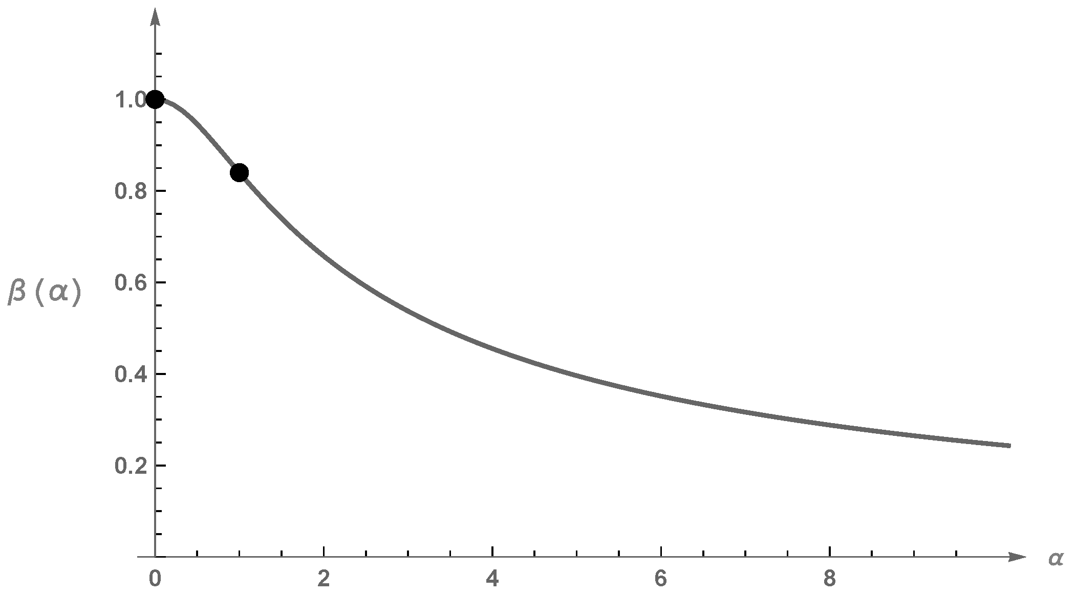
Finally, the boundary condition implies
For every given , by Lemma A1 proved in the Appendix A, the equation admits a unique negative solution . Therefore, if (see Figure 1), then the differential equation with boundary conditions (10) admits the unique solution given by (20) with . This completes the proof. □
4. The Solution
In this section, we verify that the solution V to the HJB equation found in Section 3 is indeed solution to the optimal stopping problem (3). This is a needed verification as we remind that the HJB equation represents only a necessary condition for the solution to the optimal stopping-time problem, but it is not a sufficient condition.
Theorem 1.
Proof.
Consider the process . By the Itô formula and the definition of , it follows that
Please note that is a martingale as
is bounded.
Let be a stopping time. Since , as shown in Lemma A2 proved in Appendix A, and the variable is non-positive, as the function b is non-negative and decreasing, and since is a martingale, then, by the Optional Sampling theorem,
Hence, since this is true for any stopping time , we have that .
On the other hand, since , then , for every s in , and thus
This completes the proof. □
5. Application
In this section, we show a brief application of the results of the previous sections. The process can model a pair trading process; see [14] for a survey or [15,16] for applications using the Ornstein–Uhlenbeck process. For our purposes we assume that we have a predicting model for the process trend that is given by
with , which ensures that the function b is non-increasing for . For fitting purposes one could choose a general function b of type , with restrictions on the coefficients to ensure the decreasing property. We use (23) to simplify the calculations. In addition, we assume such that . may represent the fact that at time some information is publicly disclosed, such as the earning reports of the underlining stocks, that eliminates the pair difference.
As and , by substituting in (2), we obtain that
It can be interpreted as both the time to sell the underlying pair trading and the price of an American call option with null strike price derived on the underlying pair trading process.
6. Discussion
The relevance of Theorem 1 is in that it proves the existence of a class of Itô diffusion processes for any specified (decreasing) optimal stopping boundary function b and gives the explicit expression of the corresponding value function (3). This provides a flexible model for the optimal liquidation time, i.e., the optimal time at which the investor should liquidate a position to maximize the gain, when the investor owns, or decides to include, additional information on the future trend of the underlining stock.
As an example, we can find the class of processes that have the same optimal stopping barrier of the standard Brownian bridge, i.e., with . By choosing in (23) we get the following Itô representation, for ,
It follows that multiplying by a constant factor the drift in the Itô representation of the Brownian bridge the optimal barrier has the same shape as the barrier of the Brownian bridge up to a factor equal to . For , , the process in (25) is not a Brownian bridge as, by Lemma 1, it is equal to
This class of processes is already known in the literature under the name of α-Wiener bridges, see for example [17], even if technically they are not bridges. Indeed, they cannot be generated, for , by conditioning a gaussian Itô diffusion to be equal to 0 at time 1.
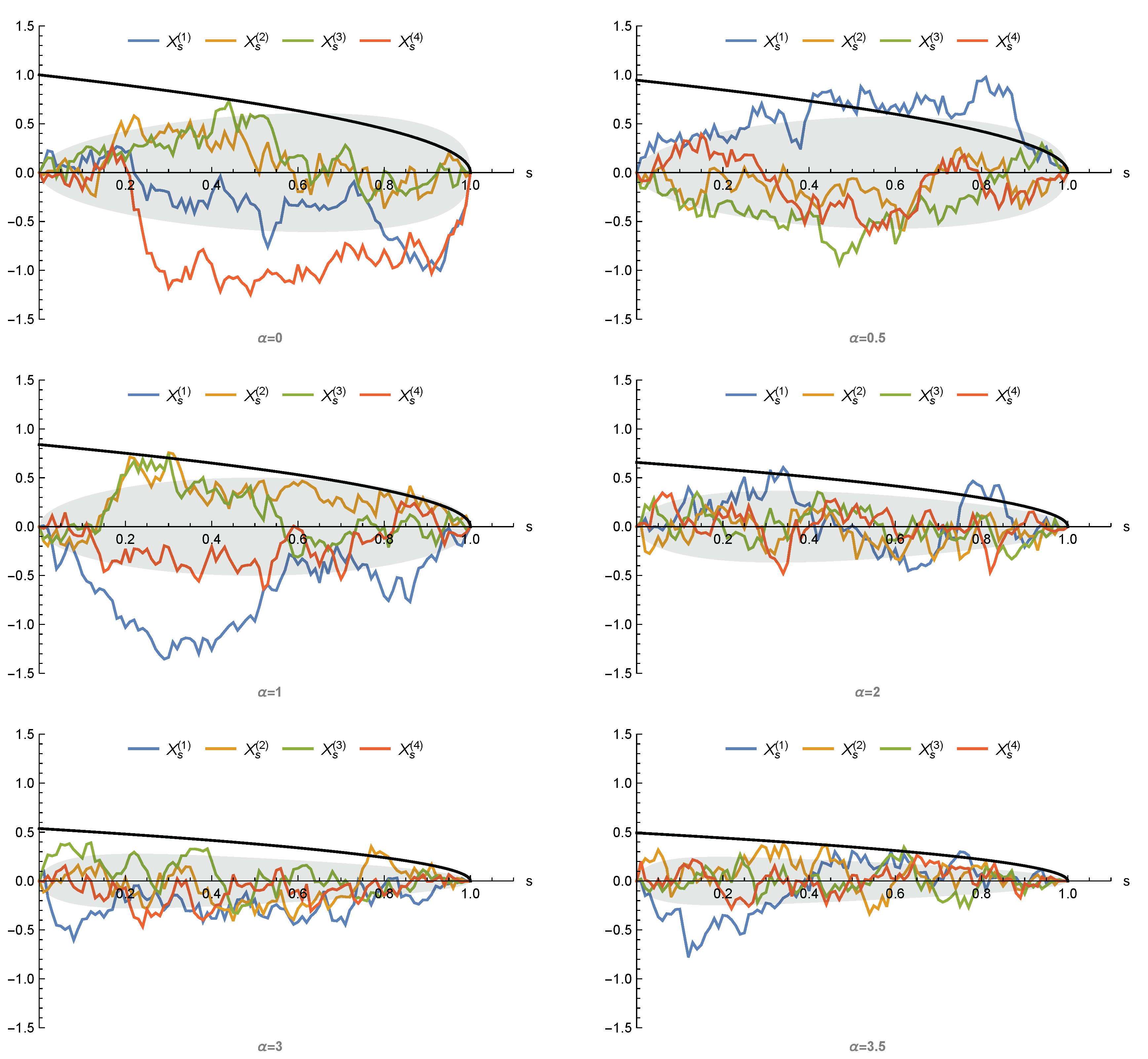
By the result above, they can be characterized by the fact that the associated optimal barrier is identical, modulo a factor, to the one of the Brownian bridge. Figure 3 gives a sample of simulations for different values of . This class provides a catalogue of alternative diffusion processes to the Brownian bridge which in practice could offer a better fitting to the data.
In the literature, the -Wiener bridges have already been used in economic settings. They appeared from the first time in [18] to model the arbitrage profit associated with some future contracts in absence of transaction costs. Then in [19,20] they were used to describe the fundamental component of an exchange rate process. For more information we refer the reader to [21] and references therein.
Author Contributions
Both authors contributed equally to this work. All authors have read and agreed to the published version of the manuscript.
Funding
This research was funded by Spanish Ministry of Economy and Competitiveness grants MTM2017-85618-P (via FEDER funds) and MTM2015-72907-EXP.
Acknowledgments
Both authors thank the NYUAD, Abu Dhabi, United Arab Emirates, for hosting them during the fall 2018.
Conflicts of Interest
The authors declare no conflict of interest.
Appendix A. Technical Lemmas
Lemma A1.
Proof.
The function is positive for and as , by (18a). The condition (A1) implies that and that the function has a critical point at . Indeed, taking derivatives we have
and equating this expression to 0 is the same as (A1).
Using (12), we have that
Computing the second derivative of at we have
and, using (A3), it follows that is a maximum point when (and it would be a minimum point when ).
Now considering , as , it follows that any critical point of is a local maximum, and therefore there cannot be more than one.
If there were two local maxima, this would imply a local minimum between them (if the function is not constant). Since , there is a unique satisfying (A1). This completes the proof. □
Lemma A2.
Any solution to (10), with , is such that , for all .
Proof.
Here we show the result without making use of Lemma 2.
If , then by the equation in (10), and thus f is convex where f is positive, and concave where f is negative. As , then f is convex in 1. Thus, f cannot touch the straight line in a point , as otherwise there would be a point such that , which is impossible as . Hence , for all .
Similarly, if is negative, for a , then f is concave in . As , for , then there would be such that , which is impossible as . Hence, , for all .
If , then by the equation in (10), . If f touches the straight line in a point , then it would exist a point such that . Hence, and so . Therefore, it would exists a local maximum , i.e., , , which is impossible as . Hence , for all .
Similarly, if is negative, as , for , there exists a local minimum , i.e., , , which is impossible as . Hence, , for all . This completes the proof. □
References
- Pikovsky, I.; Karatzas, I. Anticipative Portfolio Optimization. Adv. Appl. Probab. 1996, 28, 1095–1122. [Google Scholar] [CrossRef]
- Liu, J.; Longstaff, F. Losing money on arbitrage: Optimal dynamic portfolio choice in markets with arbitrage opportunities. Rev. Financ. Stud. 2004, 17, 611–641. [Google Scholar] [CrossRef]
- Biagini, F.; Oksendal, B. A general Stochastic calculus approach to insider trading. Appl. Math. Optim. 2005, 52, 167–181. [Google Scholar] [CrossRef]
- Avellaneda, M.; Lipkin, M.D. A market-induced mechanism for stock pinning. Quant. Finance 2003, 3, 417–425. [Google Scholar] [CrossRef]
- Ni, S.X.; Pearson, N.D.; Poteshman, A.M. Stock price clustering on option expiration dates. J. Financ. Econ. 2005, 78, 49–87. [Google Scholar] [CrossRef]
- Jeannin, M.; Iori, G.; Samuel, D. Modeling stock pinning. Quant. Finance 2008, 8, 823–831. [Google Scholar] [CrossRef]
- Avellaneda, M.; Kasyan, G.; Lipkin, M.D. Mathematical models for stock pinning near option expiration dates. Commun. Pure Appl. Math. 2012, 65, 949–974. [Google Scholar] [CrossRef]
- Shepp, L. Explicit solutions to some problems of optimal stopping. Ann. Math. Statist. 1969, 1, 993–1010. [Google Scholar] [CrossRef]
- Ekström, E.; Wanntorp, H. Optimal stopping of a Brownian bridge. J. Appl. Probab. 2009, 1, 170–180. [Google Scholar] [CrossRef] [Green Version]
- Baurdoux, E.J.; Chen, N.; Surya, B.A.; Yamazaki, K. Optimal double stopping of a Brownian bridge. Adv. Appl. Probab. 2015, 4, 1212–1234. [Google Scholar] [CrossRef] [Green Version]
- Ekström, E.; Lindberg, C.; Tysk, J. Optimal Liquidation of a Paris Trade. Adv. Math. Methods Finance 2011, 4, 247–255. [Google Scholar] [CrossRef] [Green Version]
- Peskir, G.; Shiryaev, A. Optimal Stopping and Free-Boundary Problems, 1st ed.; Birkhauser Verlag AG: Basel, Switzerland, 2006. [Google Scholar]
- Abramowitz, M.; Stegun, I. Handbook of Mathematical Functions with Formulas, Graphs, and Mathematical Tables, 1st ed.; Dover: New York, NY, USA, 1964. [Google Scholar]
- Krauss, C. Statistical Arbitrage Pairs Trading Strategies: Review and Outlook. J. Econ. Surv. 2017, 31, 513–545. [Google Scholar] [CrossRef]
- Lindberg, C. Pairs Trading with Opportunity Cost. J. Appl. Probab. 2014, 51, 282–286. [Google Scholar] [CrossRef]
- Leung, T.; Li, X. Optimal Mean Reversion Trading with Transaction Costs and Stop-Loss Exit. Int. J. Theor. Appl. Finance 2015, 18, 1550020. [Google Scholar] [CrossRef] [Green Version]
- Mansuy, R. On a one-parameter generalization of the Brownian bridge and associated quadratic functionals. J. Theor. Probab. 2004, 17, 1021–1029. [Google Scholar] [CrossRef]
- Brennan, M.; Schwartz, E. Arbitrage in Stock Index Futures. J. Bus. 1990, 63, S7–S31. [Google Scholar] [CrossRef]
- Trede, M.; Wilfling, B. Estimating exchange rate dynamics with diffusion processes: an application to Greek EMU data. Empir. Econ. 2007, 33, 23–39. [Google Scholar] [CrossRef] [Green Version]
- Sondermann, D.; Trede, M.; Wilfling, B. Estimating the degree of interventionist policies in the run-up to EMU. Appl. Econ. 2011, 43, 207–218. [Google Scholar] [CrossRef] [Green Version]
- Barczy, M.; Igloi, E. Karhunen-Loeve expansions of alpha-Wiener bridges. Cent. Eur. J. Math. 2011, 9, 65–84. [Google Scholar] [CrossRef]
Figure 1.
Plotting as a function of . The marked points are and .

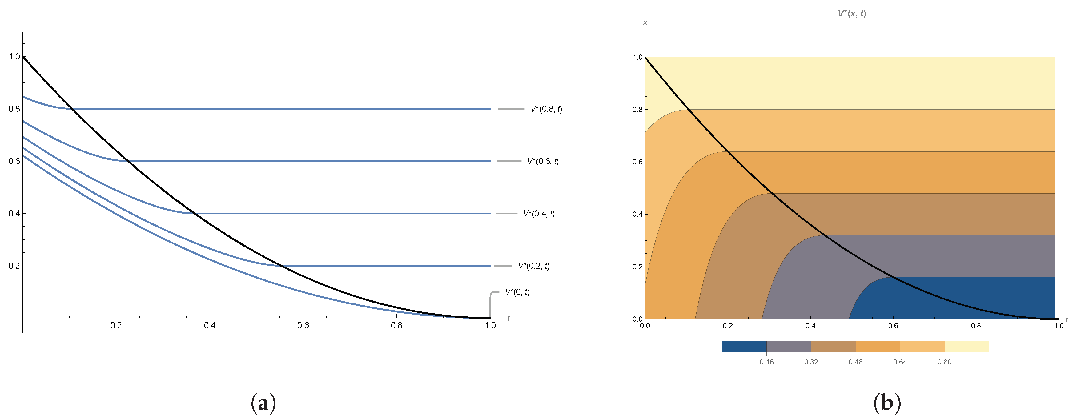
Figure 2.
Plots of the value function , computed as in (22) associated with the process in (24) for d = 2 and . The black curves represent the optimal stopping boundary . (a) as a funtion of for fixed values of . (b) as a funtion of .

Figure 3.
Four simulations of , , as defined in (26) with , , for six different values of . The light grey areas represent one standard deviation of above and below its expected value (null in the simulations). The black solid curves represent the optimal stopping boundaries.
Figure 3.
Four simulations of , , as defined in (26) with , , for six different values of . The light grey areas represent one standard deviation of above and below its expected value (null in the simulations). The black solid curves represent the optimal stopping boundaries.

© 2020 by the authors. Licensee MDPI, Basel, Switzerland. This article is an open access article distributed under the terms and conditions of the Creative Commons Attribution (CC BY) license (http://creativecommons.org/licenses/by/4.0/).
Share and Cite
MDPI and ACS Style
D’Auria, B.; Ferriero, A. A Class of Itô Diffusions with Known Terminal Value and Specified Optimal Barrier. Mathematics 2020, 8, 123. https://0-doi-org.brum.beds.ac.uk/10.3390/math8010123
AMA Style
D’Auria B, Ferriero A. A Class of Itô Diffusions with Known Terminal Value and Specified Optimal Barrier. Mathematics. 2020; 8(1):123. https://0-doi-org.brum.beds.ac.uk/10.3390/math8010123
Chicago/Turabian StyleD’Auria, Bernardo, and Alessandro Ferriero. 2020. "A Class of Itô Diffusions with Known Terminal Value and Specified Optimal Barrier" Mathematics 8, no. 1: 123. https://0-doi-org.brum.beds.ac.uk/10.3390/math8010123
Note that from the first issue of 2016, this journal uses article numbers instead of page numbers. See further details here.