Parameter and State Estimation of One-Dimensional Infiltration Processes: A Simultaneous Approach


Department of Chemical & Materials Engineering, University of Alberta, Edmonton, AB T6G 1H9, Canada
*
Author to whom correspondence should be addressed.
Mathematics 2020, 8(1), 134; https://0-doi-org.brum.beds.ac.uk/10.3390/math8010134
Submission received: 13 December 2019
/
Revised: 12 January 2020
/
Accepted: 12 January 2020
/
Published: 16 January 2020
(This article belongs to the Special Issue Mathematics and Engineering)
Abstract
:The Richards equation plays an important role in the study of agro-hydrological systems. It models the water movement in soil in the vadose zone, which is driven by capillary and gravitational forces. Its states (capillary potential) and parameters (hydraulic conductivity, saturated and residual soil moistures and van Genuchten-Mualem parameters) are essential for the accuracy of mathematical modeling, yet difficult to obtain experimentally. In this work, an estimation approach is developed to estimate the parameters and states of Richards equation simultaneously. In the proposed approach, parameter identifiability and sensitivity analysis are used to determine the most important parameters for estimation purpose. Three common estimation schemes (extended Kalman filter, ensemble Kalman filter and moving horizon estimation) are investigated. The estimation performance is compared and analyzed based on extensive simulations.
1. Introduction
Water and food scarcities are becoming serious issues worldwide due to population growth and climate change. According to United Nations statistics [1], approximately 70% of all available fresh water is consumed for agricultural activities, with the main consumer being irrigation. Currently, the average water-use efficiency in irrigation worldwide is about 50% as reported in Fischer et al. [2]. Therefore, it is of vital importance to improve irrigation water-use efficiency, in order to address the water crisis. Currently, it is still a common practice to use open-loop irrigation, which leads to excessive consumption of water resources. Closed-loop irrigation is a promising alternative to reduce water consumption and to better maintain the health of crops [3]. In the development of such a closed-loop irrigation system, it is important to have the soil moisture information of the entire field, which is in general very difficult to obtain. One way to overcome this challenge is to estimate the field’s soil moisture based on limited sensor measurements. However, this depends on the accuracy of the agro-hydrological model. In this work, we aim to develop a systematic parameter and state estimation scheme that can provide accurate estimates of soil moisture.
Specifically, in this work, we consider simultaneous state and parameter estimation based on agro-hydrological systems modeled using the Richards equation, which describes soil water dynamics. Richards equation is a partial differential equation (PDE) which falls in the family of porous medium equation (PME). The estimation and control problems of this kind of equation were widely studied in chemical engineering [4,5,6,7] and meteorology [8,9]. The Richards equation is essentially composed of the continuity equation and Darcy’s law, which is incorporated with two algebraic equations of hydraulic conductivity and capillary capacity (derivative of soil-water retention curve) [10]. The parameters of Richards equation are related to soil properties. Different approaches have been developed to estimate soil properties. Soil properties may be estimated in a soil lab by directly fitting the soil-water retention curve and hydraulic conductivity curve using collected field data of soil moisture, hydraulic conductivity and corresponding capillary pressure head [10]. However, soil properties may change over time and it would be expensive to take frequent soil samples for lab analysis especially when a big field is considered. Moreover, the hydraulic conductivity is difficult to measure. As an alternative to direct lab analysis soil parameters can be estimated indirectly based on the Richards equation and some easily-accessible field measurements such as soil moisture or capillary pressure head by minimizing the difference between measured values and model predicted values. This type of indirect approaches are referred to as inverse estimation [11]. Inverse estimation has been widely applied and its applications can be generally classified into two groups: methods based on measurements observed from one-step or multi-step outflow experiments [12,13,14,15] or methods based on time-series in-situ measurements [16,17,18,19,20]. These inverse estimation methods can only estimate soil parameters but not soil moisture or capillary pressure head. Moreover, they are mainly applicable to pre-collected datasets and cannot be used for online parameter estimation.
Sequential data assimilation is another widely used approach in estimating soil parameters online, which only requires the current measurement and prior knowledge of the system. In general, it consists of two steps, which are prediction and update steps. In the first step, a dynamical system model is initialized to describe a real process. Due to the limited knowledge about the process, the model may not predict the process accurately. Then, in the update step, an algorithm is designed to determine how to correct the prediction, based on field measurements and the dynamical model. Moreover, sequential data assimilation has the ability to deal with uncertainties in the measurements and the model. Particle filters (PF) [21], extended Kalman filters (EKF) [22] and ensemble Kalman filters (EnKF) [23,24,25,26,27] are common and widely used algorithms in sequential data assimilation for soil parameter estimation. Li and Ren [23] studied parameter estimation by augmenting parameters as states and used EnKF as the estimation algorithm. They also studied the possible factors that affect the performance of EnKF. In Reference [24], dual ensemble Kalman filter (DEnKF) was used to first estimate the states using a standard KF and then to estimate the parameters using an unscented Kalman filter. In Reference [25], two EnKFs were used to estimate the states and parameters, separately, which neglected the complex nonlinear interaction between states and parameters. In Reference [26], the authors compared three ensemble-based simultaneous state and parameter estimation methods, augmented ensemble Kalman filter, DEnKF and simultaneous optimization and data assimilation (SODA) to improve the soil moisture estimation accuracy. It concluded that the augmented EnKF was the most robust method for general conditions and SODA was better at handling complex conditions. However, it was pointed out that SODA required the highest computational resources.
However, one limitation of the above discussed methods is that they cannot handle constraints on the states or parameters and the estimation performance deteriorates when the noise is not Gaussian or the initial guess is not good. Constraints on the states and parameters are important information and may be used to significantly improve estimation performance as will be demonstrated in the simulations of this work. To address the above discussed problem, we can consider the optimization based moving horizon estimation (MHE) method, which is widely used in state estimation of nonlinear systems with explicit constraints taken into account [28,29,30].
In this work, we first introduce the investigated system and the formulation of the mathematical model in Section 2. The formulations of the estimation methods, MHE, EKF and EnKF for the augmented system are introduced in Section 3. Section 4 includes the methods of identifiability and sensitivity, used to study the significance of parameters. Section 5 shows the synthetic experimental setup, determination of significant parameters and MHE estimation results compared with EKF and EnKF, followed by concluding remarks in Section 6. Some preliminary results of this work were reported in Reference [31]. Compared with Reference [31], this paper provides significantly expanded explanations and significantly extended simulation results.
2. System Description and Problem Formulation
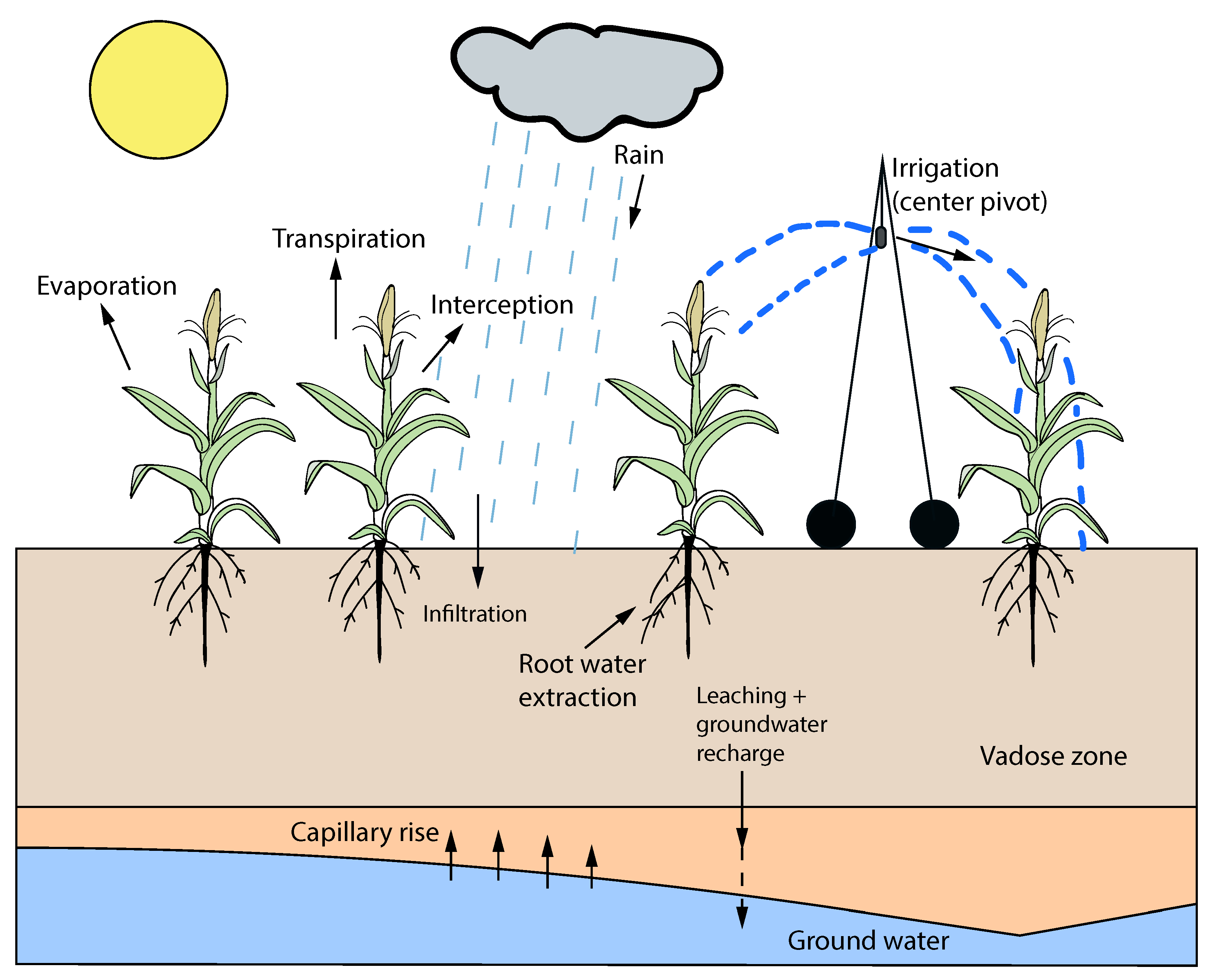
An agro-hydrological system describes the water movements between soil, crop and atmosphere. Figure 1 shows a schematic of an agro-hydrological system, which is a modified version from Reference [32]. The water movements usually involve water transportation within the soil, root water extraction, transpiration and evaporation from the soil and leaves to the air and precipitation including rain and irrigation.
In this work, we focus on soil that is above the water table (i.e., soil in the vadose zone). Within the vadose zone, the water movement is mainly driven by capillary and gravitational forces and the water dynamics can be modeled using Richards equation under the assumptions: (1) soil properties are spatially homogeneous within the system; (2) irrigation is uniformly applied on the surface of the system; and (3) the horizontal water dynamics are much smaller than the vertical dynamics due to the gravity force and the horizontal water dynamics can be neglected. Then, the 1D Richards equation modeling the vertical water dynamics is shown below [33]:
In Equation (1), h (m) is the capillary potential in the unsaturated soil, (m/s) and (1/m) denote hydraulic conductivity and capillary capacity of the soil, respectively. Note that in Richards equation, the value 1 on the right-hand-side denotes the impact of gravitational force on water in the vertical direction. The upward z-direction is defined as the positive direction. The van Genuchten-Mualem soil hydraulic model and , as functions of the capillary potential h, are shown as follows [10]:
where (m/s), and are saturated hydraulic conductivity, saturated soil moisture and residual soil moisture, respectively. The van Genuchten-Mualem parameters (1/m) and n characterize the properties of the soil, which are proportional to the inverse of the soil air entry pressure and of soil porosity, respectively. These two closed-form expressions are derived by van Genuchten based on his expression of soil-water retention curve and Mualem’s open-form expression of hydraulic conductivity. Since Mualem’s expression is not studied further, in this work, only van Genuchten’s soil-water retention equation is shown below [10]:
where denotes volumetric water content in soil.
The five parameters , , , n and determine the properties of a type of soil. With sufficient soil samples, , , and n can be estimated by fitting the soil-water retention curve Equation (4) utilizing soil moisture and capillary potential data sets. Then can be estimated by fitting hydraulic conductivity and capillary potential data sets into Equation (2). By using this approach, we can only get a snapshot of the soil properties at one time instant, however, soil properties do slowly change over time due to agricultural activities [34]. While the experiments can be repeated to get parameter estimates at different times, it is very time consuming and expensive, especially when the investigated field is large and has various soil types over the field. Therefore, online state and parameter estimation based on ease-to-access field measurements provides a favorable approach to estimate soil properties.
In this work, we study the estimation of soil properties based on real-time field measurements: capillary potential h.
Finite Difference Model Development
Richards equation is a nonlinear partial differential equation (PDE) with respect to both the temporal and spatial variables. Because of its complex structure, it is difficult to have a closed-form solution. Therefore a finite difference method is implemented to find a numerical approximation of its solution. Two-point forward difference scheme and two-point central difference scheme are used to approximate the derivatives with respect to the temporal and spatial variables, respectively:
where and , representing time and position indices, respectively. and are the total number of time instants and states investigated. and represents compartment thickness of compartment i. The state i is at the center of the compartment i. The hydraulic conductivity, for example, , is linearized explicitly as .
The discrete-time finite difference model at node i and time instant can be obtained by substituting Equations (5) and (6) into Equation (1) as follows:
where is defined as .
The Neumann boundary condition is utilized to characterize the top and bottom boundaries of the system and are shown below, respectively:
where the subscripts T and B represent the top and bottom boundary conditions, respectively. The (m/s) is the irrigation rate which is considered as the input of the system and free drainage boundary condition is applied at the bottom.
Before introducing estimation methods, for the sake of simplicity, we obtain the compact form of the model by combining Equation (7) for all spatial nodes and the boundary conditions, Equations (8) and (9). It is shown below:
where represents the state vector containing capillary pressure values for corresponding spatial nodes, at the defined time instant k. , represents the parameter vector containing the parameters to be estimated. , denote the input and the model disturbances, respectively.
The general output function, with the measurement noise taken into account, is shown below:
where and denote the measurement vector and measurement noise. If the volumetric soil moisture is measured by the soil moisture sensor, Equation (11) is the general form of Equation (4). On the other hand, if tensiometers are used to measure the water potential h in the soil, Equation (11) simply represents a matrix indicating which states are measured by the tensiometers.
Furthermore, in order to estimate the states and parameters simultaneously, the parameter vector is augmented at the end of the state vector and treated as a part of the augmented state vector, . An estimation of the augmented state vector X brings the benefit to estimate the states and parameters at the same time. The augmented model can be constructed by augmenting Equation (10) with the following equation:
where . When the parameter vector p is assumed to be constant during the study, is equal to 0.
At last, the augmented model and output function used for simultaneous parameter and state estimation are shown below:
where , and the subscript a of and denotes the augmentation.
3. Estimation Methods
In this work, three common estimation schemes, MHE, EKF and EnKF are applied to the augmented model to estimate the states and parameters. The design of these methods are detailed next.
3.1. Moving Horizon Estimation
MHE is an online optimization based estimation method [28]. The MHE optimization problem used in this work is formulated as follows:
In the MHE optimization, the objective is to minimize the distance between the predicted and observed measurements which is measured by the term as shown in Equation (14), where the term is defined in Equation (16). The caret sign^indicates that the variable is estimated. The model uncertainty or the process disturbance is taken into account and represented by , where the term is defined in Equation (15). The arrival cost, summarizes the information from the initial state of the model up to the beginning of the estimation window of the MHE. N denotes the length of the estimation window. After each optimization, only the last estimated state within the estimation window is used. and within the moving window are the decision variables of the optimization problem. The term follows the definition of Equation (17). represents the estimated state at time instant , which is estimated at time instant . Matrices P, Q, R are positive definite matrices and they are the covariance matrices of state uncertainty, process noise and measurement noise , respectively. In addition, MHE takes into account constraints on the states, parameters and model uncertainties as expressed in Equations (18) and (19).
3.2. Extended Kalman Filter
EKF is a common method used for state estimation of nonlinear systems based on successively linearizing the nonlinear system. It can be divided into two steps, which are prediction and update steps. The prediction step predicts the state X and the state covariance matrix P. When a new measurement is available, the Kalman gain K is calculated first and then X and P are updated. The detailed steps are shown below:
- Prediction step
- (a)
- State prediction:The model disturbance are not propagated as the states and parameters. Instead, it is explicitly included in the state covariance prediction.
- (b)
- State covariance prediction:where and Q is the covariance matrix of the model disturbance .
- Update step
- (a)
- Kalman gain calculation:where and R is the covariance matrix of the measurement noise .
- (b)
- State update:The augmented state and parameter vector X is updated when a new measurements is available.
- (c)
- State covariance update:State covariance matrix P is updated. I is the identity matrix with dimension .
3.3. Ensemble Kalman filter
The EnKF is a method developed by Evensen [35] based on Monte Carlo method. An ensemble of trajectories of the system is generated based on the priori probability distribution of the case. A practical implementation scheme which estimated the probability distribution based on the information embedded within ensembles, instead of propagation of the state covariance matrix P, is discussed in Reference [36]. Unlike EKF, it directly utilizes the nonlinear model Equation (13), which does not require frequent model linearization. In addition, the model disturbance and measurement noise are taken into account at the same time as the states and parameters propagate. It starts with generating the ensembles, then follows with the two steps as the same as in EKF.
- 1.
- Initialization step
- (a)
- Generating ensembles:where an ensemble containing M initial states , , is generated and m is the index of the ensemble. The ensemble follows the multivariate normal distribution with mean, and covariance matrix of the initial state, .
- 2.
- Prediction step
- (a)
- State prediction:where . Just like generating the ensemble of , a normally distributed set of are generated with the mean 0 and the covariance matrix Q. Overall M trajectories propagate, with model disturbance explicitly considered.
- 3.
- Update step
- (a)
- Kalman gain calculation:where, and . is the cross-covariance matrix of the state and measurement vectors and is the auto-covariance matrix of the measurement vector. The mean of the state or measurement vector is calculated based on the corresponding ensembles.
- (b)
- State update:where . All M state vectors are updated, when the new measurement is available. The measurement uncertainty is taken into account by generating a normally distributed ensemble of measurement noises , which has mean 0 and covariance matrix R. At last, the estimated state is obtained as the mean of the corresponding ensembles , .
4. Proposed Procedure to Determine Significant Parameters and Number of Sensors
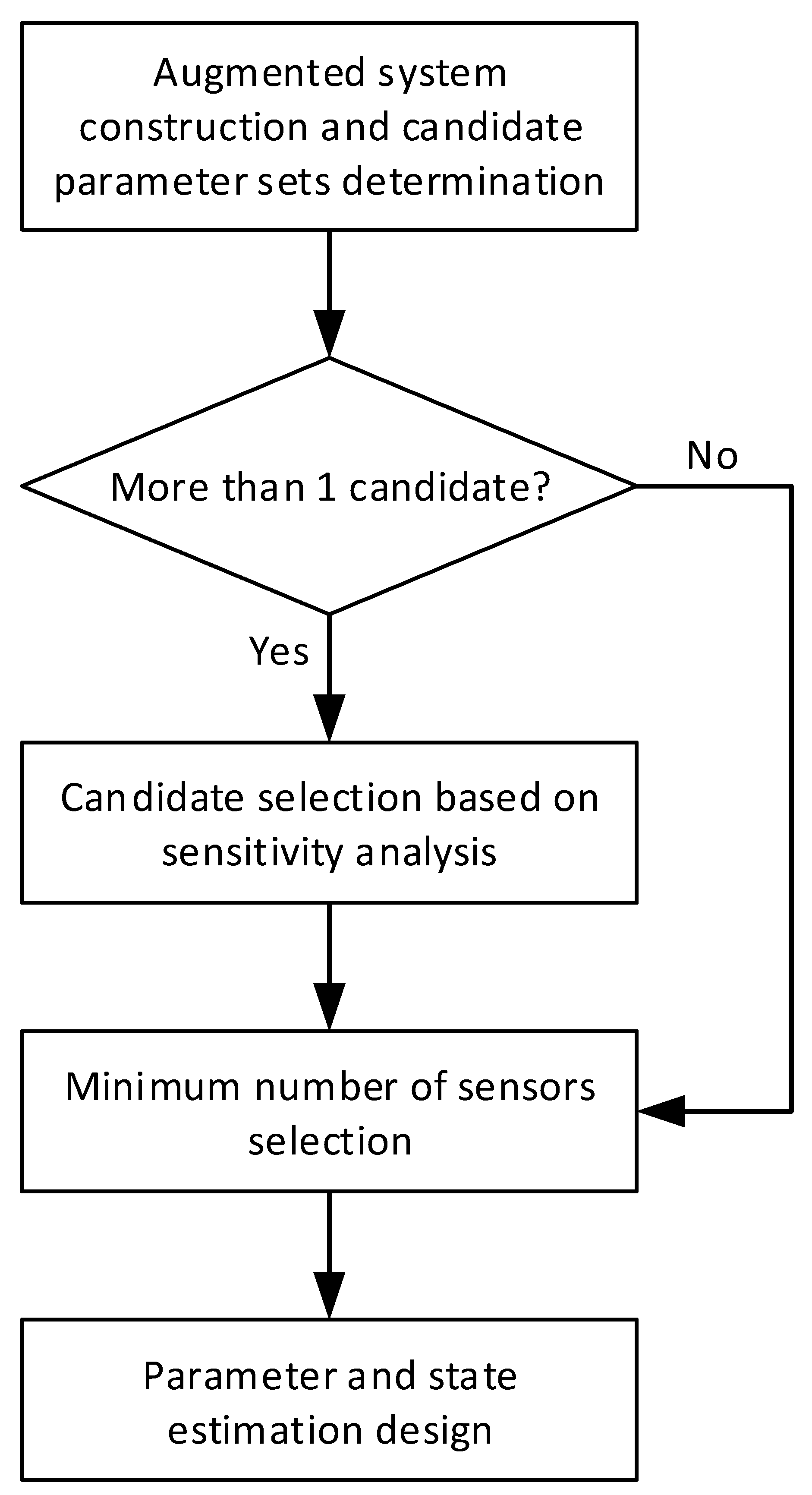
In reality, it is nearly impossible to measure all states and the parameters can not be determined easily. First, according to Reference [37], it states that the original system of Equation (10) is observable using limited number of measurements. That means the states can be recovered. However, for this work the augmented system of Equation (13) is studied. For this case, it is necessary to ensure that the parameters are also identifiable since they are estimated with the states simultaneously. The proposed procedure to check the identifiability of the parameters, to select appropriate parameters for estimation and to determine the minimum number of sensors is shown in Figure 2. The key steps are explained below.
4.1. Determine Candidate Parameter Sets for Estimation
After augmenting the original nonlinear system with the parameters, the entire system may not be observable. In order to determine which parameters can and should be estimated online, we resort to observability analysis [38]. In this step, we assume that all the soil moisture states are measured; that is, . This ensures that the observability analysis results depend only on the parameters. If the augmented system is not observable, then the unobservability is caused by the augmentation of the parameters in the state vector.
When checking the observability of the augmented system, we start with the system with all the parameters augmented. If the augmented system is not observable, then one of the parameters is removed from the augmented system. If there are parameters, then there are different ways to remove the one parameter. All these cases are considered. If after removing one parameter and upon finding that the new augmented system is observable, we continue to the next step to determine which parameter set to estimate (described in the next subsection). If we can still not find an observable augmented system after removing one parameter, we continue to remove two parameters from the original augmented system. Again, all the possible cases should be considered. If we can still not find an observable system, we continue to remove three parameters from the original augmented system. This continues until we find at least a system that is observable.
When checking the observability, we propose to use the Popov-Belevitch-Hautus (PBH) observability theory. Other observability tests may also be used. Since the augmented system is a nonlinear system, it should be linearized before PBH can be applied. It is recommended that instead of linearizing the system at one point, it should be linearized at different point along typical operating trajectories as used in Reference [39].
Note that the observability analysis described in this step may generate more than one candidate parameter sets that can be estimated through augmentation of the original agro-hydrological system.
4.2. Sensitivity Analysis
If there is only one candidate parameter set from the previous step, we can continue with the candidate and move to the next subsection to find the minimum number of sensors. However, if there are more than one candidates, we need to determine which parameter set to choose. We propose to use sensitivity analysis to determine the importance of these parameters and pick the set containing the most important parameters for further analysis.
The sensitivity analysis measures how the outputs respond when there is a change in one parameter. The sensitivity matrix shown below contains the information about, at time instant k, how each output is affected by which is constituted of the initial state and the parameters p.
The detailed steps to derive the sensitivity matrix is explained below and is inspired by Reference [40]. When performing this sensitivity analysis, we consider the augmented system of Equation (13) without considering the disturbance and but with explicitly expressed as shown below:
where is considered as an independent variable.
The objective is to check how a change in the initial state and the parameters p affects the prediction error e, which comes from the difference between the predicted y and the observed measurements . We can represent this as:
Because the observed measurement is not affected by the initial state and parameters, the above expression is simplified as below:
Equation (22) can be derived by taking the partial derivative of Equation (20) with respect to the augmented state vector . And the sensitivity equations with respect to are shown below:
Because the intermediate variable depends on the independent variable as well, the chain rule is applied on the right hand sides of Equation (23) and we can further get that
By defining and , the above equations can be converted to ordinary differential equations, which are shown below:
Therefore, by giving the initial states of Equations (20) and (25) and solving them at the same time, the sensitivity matrix can be obtained. may be normalized to obtain the normalized sensitivity matrix :
Once the sensitivity matrix is obtained, we can use it to determine the relative importance of different parameters. Specifically, we can exam the magnitudes of the elements in the sensitivity matrix. Each parameter corresponds to one column in the sensitivity matrix. We can use, for example, the summation of the absolute values of the elements of each column to compare the relative importance of parameters. A bigger value implies a more important parameter in terms of its impact on the outputs. Among all the candidate parameter sets, we keep the parameter set with the highest sensitivity values.
4.3. Minimum Number of Sensors
After the parameter set to be estimated is determined, the original system is augmented with the parameters, as illustrated in Reference [37], we can use the maximum multiplicity theory [41] to determine the minimum number of sensors required to ensure the observability of the entire system. Then, state estimation techniques can be used to estimate the states and parameters simultaneously.
5. Simulation Results and Discussion
5.1. System Description
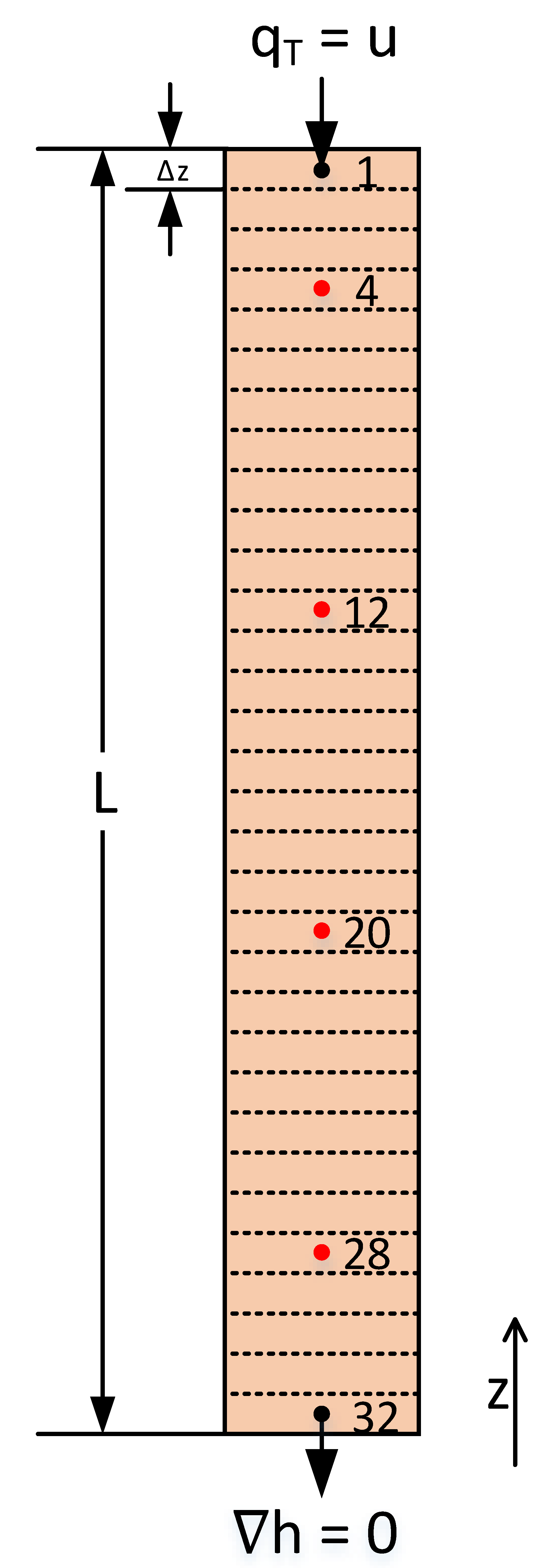
In this work, a total length (L) of 67 cm loam soil column is investigated, which is shown in Figure 3. The soil column is equally partitioned into 32 compartments. Correspondingly, Richards equation is spatially discretized into 32 states () in the z-direction, with each state centered at the corresponding compartment. At the surface of the soil, the irrigation, , is performed at the rate of 2.50 cm/day, from 12:00 PM to 4:00 PM daily. At the bottom, the free drainage boundary condition is used, which means the gradient between the last state and the state at the bottom boundary is 0. The soil column has the homogeneous initial condition of −0.514 m capillary pressure head and the parameters of the soil are shown in Table 1 [42].
5.2. Determination of Significant Parameters and Number of Sensors
The augmented system (Equation (13)) is utilized to achieve simultaneous parameter and state estimation. First without knowing the observability of the augmented system, all 5 parameters (, , , and n) are augmented; that is, . In addition, all 32 states are assumed to be measured. A 10-day state trajectory, without considering the process and measurement noise, is used in the rest of the subsection for selecting appropriate parameters for estimation and determining the minimum number of sensors. It is assumed that the measurements are available every 1 h.
Following the procedure as discussed in Section 4.1, we apply the PBH observability test on the augmented system to check the identifiability of the parameters. The test is conducted every sampling time, which requires the system to be linearized accordingly. According to the results, the augmented system is not observable. This implies that it is impossible to identify the 5 parameters simultaneously. In order to look for an observable system, parameters are removed from the augmented system. We start with removing only 1 of the parameters and this results in 5 different augmented systems with each one augmented with 4 parameters. Then, the observability of the 5 augmented systems is checked. It was found that 2 of the 5 systems are observable. In these two systems, either or is removed. Since observable systems are found, we proceed to the next step to determine the final parameter set.
To determine which parameter set to use, the significance of and is compared based on the sensitivity analysis described in Section 4.2. Sensitivity analysis is conducted based on the original augmented system with all the parameters. The initial state of Equation (25) is an identity matrix of size . By comparing the summation of the absolute values of the elements of each column of the normalized sensitivity matrices , it can be found that the summation corresponding to the column (82,674) is much bigger than the one for (14,997). Based on this, is considered as a more important parameter because it has more impact on the output than . Therefore, the parameter set containing is removed and the final parameter set will be used in the remaining analysis is .
In the above analysis, it was assumed that all the states (soil moisture) are measured for the purpose of determining the parameters for estimation. When the set of parameters is determined, we remove this assumption to determine the minimum number of sensors (measurements) needed to ensure the observability of the augmented system with 4 parameters. Following the method described in Section 4.3, the maximum multiplicity method is conducted, and it can be found that the minimum number of sensors is 4.
5.3. Simultaneous Parameter and State Estimation
According to the minimum number of sensors found above, it is assumed that 4 tensiometers () are installed. Specifically, we assume that these sensors are installed at 7.30 cm, 24.1 cm, 40.8 cm and 57.6 cm below the surface, which measure the 4th, 12th, 20th and 28th states, respectively. In the simulations, the actual parameter values used are shown in Table 1 and they are assumed to be constant within the investigated temporal domain. Process noise and measurement noise and are considered in the simulations and they have zero mean and standard deviations m and m, respectively.
In the design of the state and parameter filters (EKF, EnKF) and estimator (MHE), the model augmented with 4 parameters (, , and n) is used. The initial guesses of the initial states and parameters in the filters and estimator are listed in Table 2 and compared with those used in the actual system.
For the EKF and EnKF, the weighting matrices Q and R are designed as the auto-covariance matrices of and with the standard deviations mentioned before. However, the diagonal elements of Q corresponding to augmented parameters are 0, because the parameters are assumed to be constant. In simulations, is used to approximate the value 0 and to ensure the positive definiteness of the matrix. The diagonal elements of P corresponding to the states are configured as the square of and those of parameters are configured as the square of . For the designed EnKF, 100 ensembles are used.
For the design of MHE, the estimation window size is selected to be 8 h. The weighting matrices P, Q, and R retain the same ratio with respect to those used in EKF and EnKF but with a much bigger magnitude to ensure the numerical stability of the associated optimization problem. In addition, the P matrix is constant for all the optimizations. The constraints of the states, parameters and the model uncertainty are listed in Table 3. The upper and lower bounds of the term are 0 because the parameters are constant.
In the following simulations, the root mean square error (RMSE) will be used to evaluate the performance of the MHE, EKF and EnKF. The estimation performance in terms of the states and parameters are evaluated separately. Their equations are shown below:
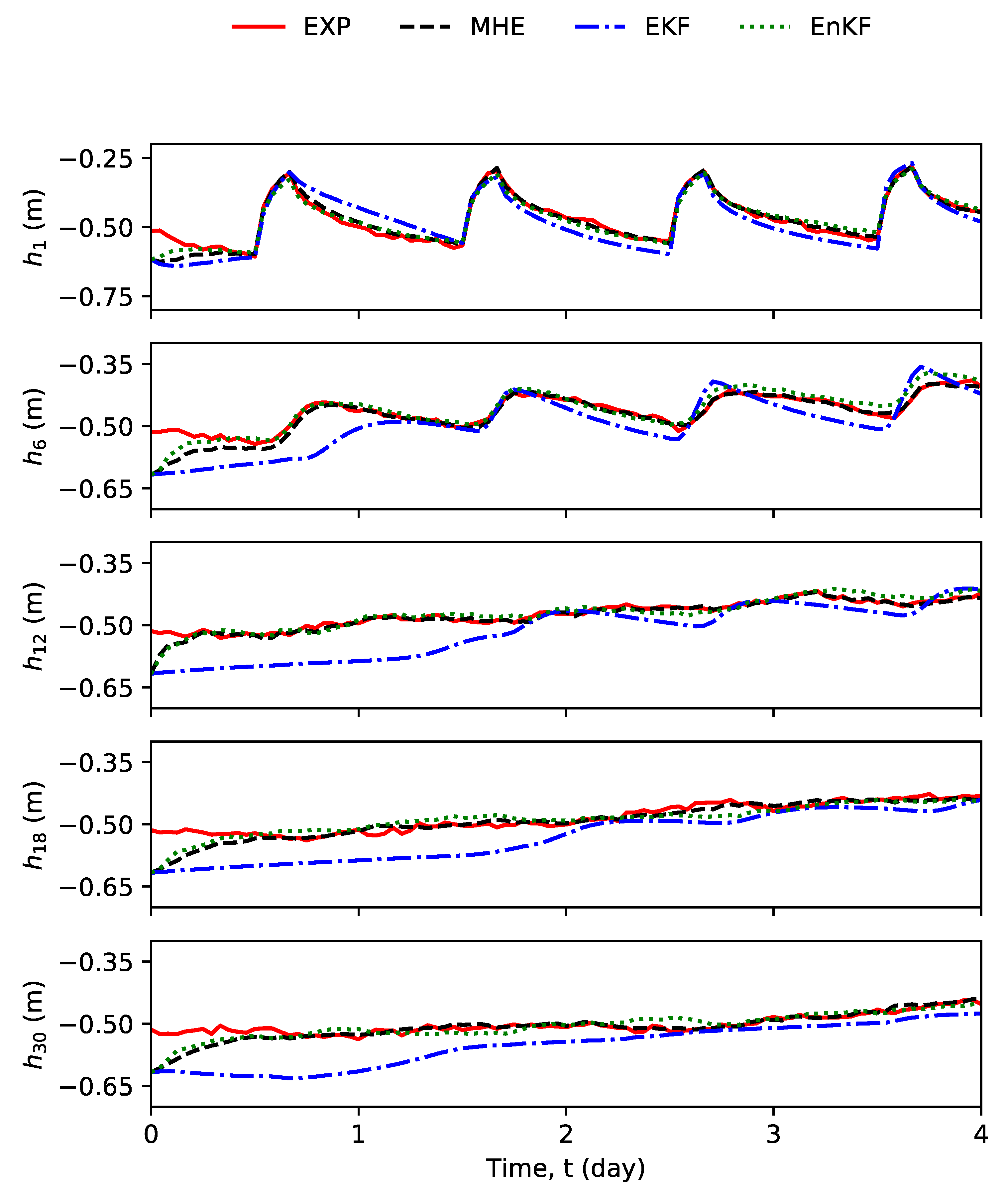
First, we performed simulations assuming that the parameter (which is not estimated) is known and is the same as the value used in the actual system. Figure 4 and Figure 5 show some representative estimated states and all the parameters using MHE, EKF and EnKF, which are also compared with their true values. Figure 4 shows the state trajectories of the top node and a few middle nodes and one bottom node. From the figure, it can be seen that the top node has more dynamics because it takes time for irrigated water to pass from the upper part and to the lower part. In terms of state estimation performance, from Figure 4, it can be seen that MHE and EnKF give very much more accurate state estimates than the EKF. Note that from Figure 4, it can also be seen that the estimates of the 12th state converge faster than the other estimates. This is because it is a sensor node.
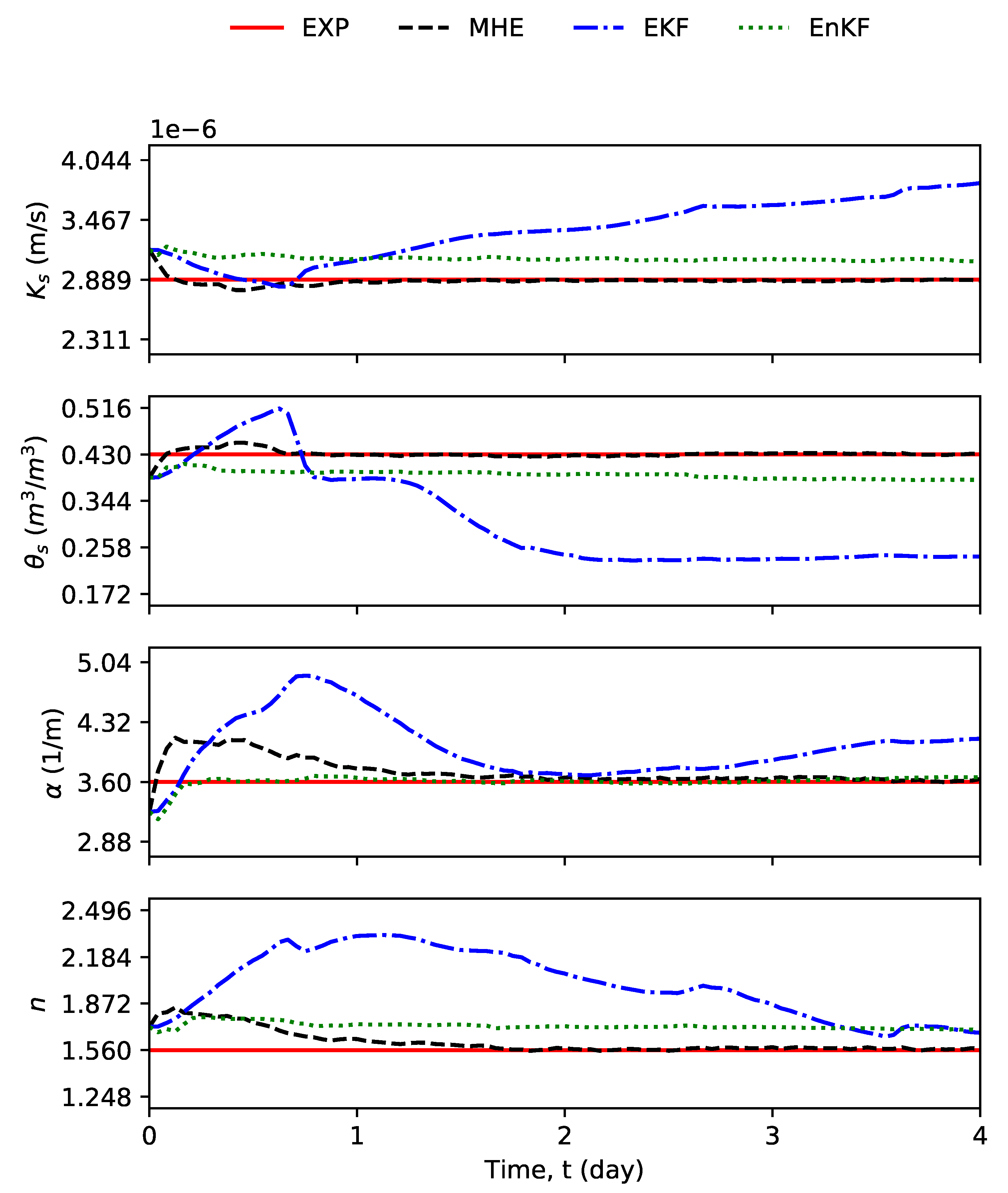
In terms of parameter estimation, Figure 5 shows the results. From the figure, it can be seen that only MHE is capable of estimating the parameters, whereas those estimated by EKF and EnKF diverge from their true values. This may be because of the constraints used in MHE. These constraints provide more useful information to MHE in addition to the measurements.
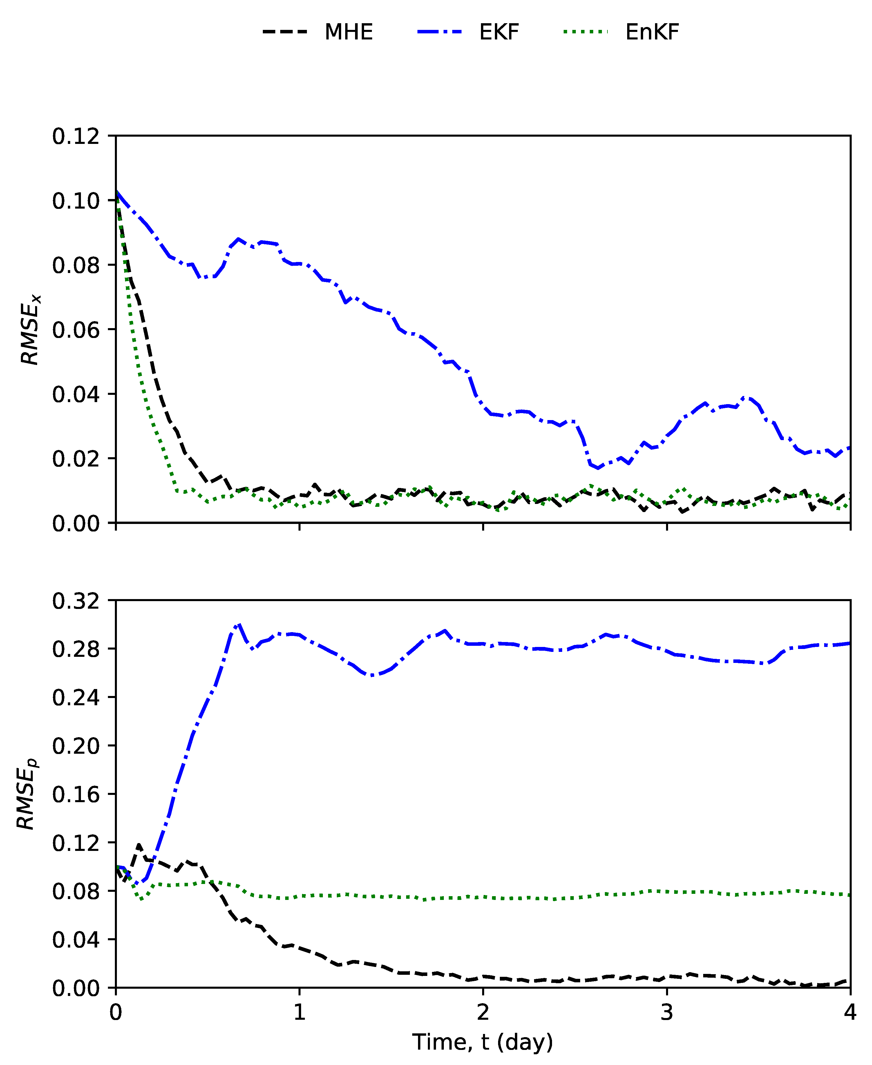
The trajectories of the performance indices and associated with the MHE, EnKF and EKF are shown in Figure 6. These trajectories further confirm that the MHE and EnKF have better performance than EKF in estimation of the states and the MHE outperforms both EnKF and EKF in parameter estimation.
In the previous set of simulations, the parameter is assumed to be accurately known and is used in the MHE, EnKF and EKF. However, this assumption may not hold in practice. In this set of simulations, we study how an inaccurate may affect the state and parameter estimation performance. In this set of simulations, the value of used in the MHE, EnKF and EKF is assumed to be 10% off from the actual value. The tuning parameters used in the filters and estimator are the same as the ones used in the previous simulations. In this case, the EnKF and EKF cannot give accurate parameter estimates as in the previous case, either. The MHE is still the only estimation method that can give good parameter estimates. Table 4 summarizes the estimated parameters using the MHE in the two sets of simulations. The reported estimated values are the mean estimated values after the estimates have converged. According to the results, a 10% difference of does not affect the estimation results of other parameters when MHE is used. This verifies that the removal of has a minor impact on the overall state and parameter estimation performance. This further implies that the proposed method in parameter selection is applicable.
In this work, the spatial heterogeneity in soil properties is not considered. When parameter heterogeneity presents, a 3D Richards equation is needed to describe the water dynamics. The studied MHE algorithm can be extended to handle heterogeneous parameters in a straightforward manner. It is expected that the weighting matrices should be tuned taking into account the spatial heterogeneity. Also, a system with different soil types may be decomposed into a few subsystems with each subsystem having the same type of soil and distributed or decentralized estimation may be used accordingly. MHE may still be used in the design of the subsystem estimators.
5.4. Effects of the Simulation Parameters
In this subsection, we further study the performance of MHE in terms of number of measurements and size of estimation window of MHE.
5.4.1. Effects of Number of Measurements
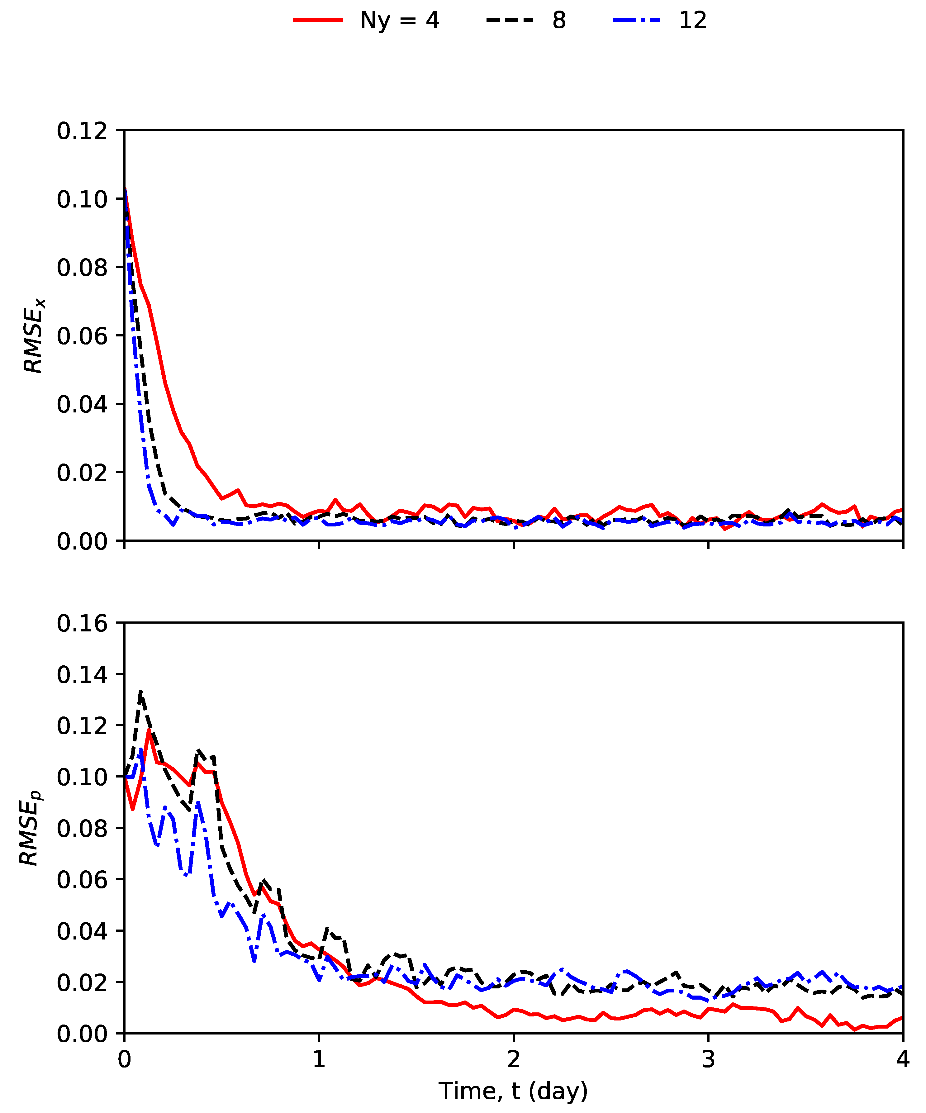
First, we study the effects of number of measurements on the estimation performance of MHE. In addition to the case with 4 measurements, we also consider cases with 8 and 12 measurements. Figure 7 shows how the two performance indices and evolve over time. From the top plot, it can be seen that the more sensors are used, the faster state estimates converge. This is because the sensors are directly measuring the states. When there are more sensors, it implies that we have more information of the states. For the parameter, there is no obvious difference between the convergence speeds with different number of measurements. Comparing the convergence speed between the state estimates and parameter estimates, the state estimates converge much faster within one day while the parameter estimates take longer time to converge (about 2 days). Overall, from this set of simulations, it can be concluded that 4 sensors are sufficient to estimate all states and parameters accurately.
5.4.2. Effects of MHE Estimation Window Size
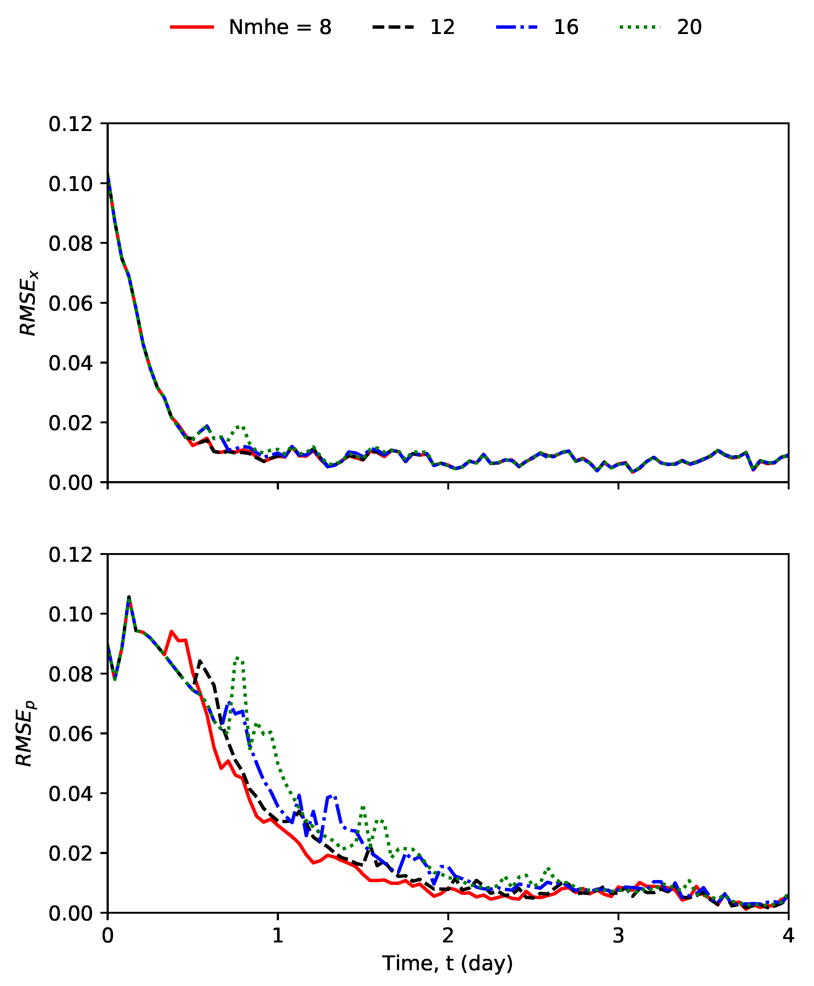
The effects of the size of the estimation window of MHE on estimation performance are also studied assuming that there are 4 measurements. Figure 8 shows how the two performance indices and evolve over time with different estimation window sizes. From the figure, it can be seen that from both plots that a window size of 8 is sufficient and further increase of the estimation window size does not bring significant performance improvement.
6. Conclusions
In this work, we have investigated simultaneous state and parameter estimation using moving horizon estimation (MHE), extended Kalman filter (EKF) and ensemble Kalman filter (EnKF) applied to an infiltration process in an agro-hydrological system. First, a procedure was proposed to find the appropriate parameter set for estimation based on the observability of the augmented system and the sensitivity of the outputs to the parameters. It was found that only 4 out of 5 parameters (hydraulic conductivity, saturated soil moisture and van Genuchten-Mualem parameters) can be considered in simultaneous state and parameter estimation. The less important parameter (residual soil moistures) was not considered in parameter estimation. After determining the parameter set for estimation, the minimum number of sensors was also found based on the maximum multiplicity theory. Simulation results showed that the MHE has an overall the best state and parameter estimation performance due to the inclusion of state and parameter constraints in the estimation. It was also found that the uncertainty in the residual soil moisture (which was not estimated) does not affect the overall estimation performance too much. The effects of number of measurements and estimation window size of the MHE were also studied through simulations. It was found that 4 measurements and a window size of 8 for MHE are sufficient to provide accurate state and parameter estimates.
Author Contributions
Conceptualization, methodology, simulation design, S.B., S.R.S. and J.L.; validation and formal analysis, S.B., S.R.S., X.Y. and J.L.; original draft preparation, S.B.; review and editing, S.B., S.R.S., X.Y., J.L. and S.L.S.; supervision, J.L. All authors have read and agreed to the published version of the manuscript.
Funding
This research was funded by Natural Sciences and Engineering Research Council of Canada (NSERC).
Conflicts of Interest
The authors declare no conflict of interest.
References
- AQUASTAT Main Database. Food and Agriculture Organization of The United Nations (FAO). Available online: http://www.fao.org/nr/water/aquastat/data/query/index.html?lang=en (accessed on 31 October 2019).
- Fischer, G.; Tubiello, F.N.; van Velthuizen, H.; Wiberg, D.A. Climate change impacts on irrigation water requirements: Effects of mitigation, 1990–2080. Technol. Forecast. Soc. Chang. 2007, 74, 1083–1107. [Google Scholar] [CrossRef] [Green Version]
- Mao, Y.; Liu, S.; Nahar, J.; Liu, J.; Ding, F. Soil moisture regulation of agro-hydrological systems using zone model predictive control. Comput. Electron. Agric. 2018, 154, 239–247. [Google Scholar] [CrossRef]
- Narasingam, A.; Siddhamshetty, P.; Kwon, J.S.I. Handling Spatial Heterogeneity in Reservoir Parameters Using Proper Orthogonal Decomposition Based Ensemble Kalman Filter for Model-Based Feedback Control of Hydraulic Fracturing. Ind. Eng. Chem. Res. 2018, 57, 3977–3989. [Google Scholar] [CrossRef]
- Aanonsen, S.I. The Ensemble Kalman Filter in Reservoir Engineering—A Review. SPE J. 2009, 14, 393–412. [Google Scholar] [CrossRef]
- Siddhamshetty, P.; Kwon, J.S.I. Model-based feedback control of oil production in oil-rim reservoirs under gas coning conditions. In Proceedings of the 2018 Annual American Control Conference (ACC), Milwaukee, WI, USA, 27–29 June 2018; IEEE: Milwaukee, WI, USA, 2018; pp. 2605–2610. [Google Scholar] [CrossRef]
- Hasan, A.; Foss, B.; Sagatun, S. Flow control of fluids through porous media. Appl. Math. Comput. 2012, 219, 3323–3335. [Google Scholar] [CrossRef]
- Bengtsson, L.; Ghil, M.; Källén, E. Dynamic Meteorology: Data Assimilation Methods; Springer: New York, NY, USA, 1981. [Google Scholar]
- Ghil, M.; Malanotte-Rizzoli, P. Data Assimilation in Meteorology and Oceanography. In Advances in Geophysics; Elsevier: Amsterdam, The Netherlands, 1991; Volume 33, pp. 141–266. [Google Scholar] [CrossRef]
- van Genuchten, M.T. A closed-form equation for predicting the hydraulic conductivity of unsaturated soils. Soil Sci. Soc. Am. J. 1980, 44, 892–898. [Google Scholar] [CrossRef] [Green Version]
- Marquardt, D.W. An algorithm for least-squares estimation of nonlinear parameters. J. Soc. Ind. Appl. Math. 1963, 11, 431–441. [Google Scholar] [CrossRef]
- Kool, J.B.; Parker, J.C.; van Genuchten, M.T. Determining soil hydraulic properties from one-step outflow experiments by parameter estimation: I. Theory and numerical studies. Soil Sci. Soc. Am. J. 1985, 49, 1348–1354. [Google Scholar] [CrossRef] [Green Version]
- Toorman, A.F.; Wierenga, P.J.; Hills, R.G. Parameter estimation of hydraulic properties from one-step outflow data. Water Resour. Res. 1992, 28, 3021–3028. [Google Scholar] [CrossRef]
- van Dam, J.C.; Stricker, J.N.M.; Droogers, P. Inverse method for determining soil hydraulic functions from one-step outflow experiments. Soil Sci. Soc. Am. J. 1992, 56, 1042. [Google Scholar] [CrossRef]
- Il Hwang, S.; Powers, S.E. Estimating unique soil hydraulic parameters for sandy media from multi-step outflow experiments. Adv. Water Resour. 2003, 26, 445–456. [Google Scholar] [CrossRef]
- Russo, D.; Bresler, E.; Shani, U.; Parker, J.C. Analyses of infiltration events in relation to determining soil hydraulic properties by inverse problem methodology. Water Resour. Res. 1991, 27, 1361–1373. [Google Scholar] [CrossRef]
- Abbaspour, K.C.; van Genuchten, M.T.; Schulin, R.; Schläppi, E. A sequential uncertainty domain inverse procedure for estimating subsurface flow and transport parameters. Water Resour. Res. 1997, 33, 1879–1892. [Google Scholar] [CrossRef] [Green Version]
- Ritter, A.; Hupet, F.; MunÄoz-Carpena, R.; Lambot, S.; Vanclooster, M. Using inverse methods for estimating soil hydraulic properties from field data as an alternative to direct methods. Agric. Water Manag. 2003, 59, 77–96. [Google Scholar] [CrossRef]
- Rashid, N.S.A.; Askari, M.; Tanaka, T.; Simunek, J.; van Genuchten, M.T. Inverse estimation of soil hydraulic properties under oil palm trees. Geoderma 2015, 241–242, 306–312. [Google Scholar] [CrossRef] [Green Version]
- Li, Y.B.; Liu, Y.; Nie, W.B.; Ma, X.Y. Inverse modeling of soil hydraulic parameters based on a hybrid of vector-evaluated genetic algorithm and particle swarm optimization. Water 2018, 10, 84. [Google Scholar] [CrossRef] [Green Version]
- Montzka, C.; Moradkhani, H.; Weihermüller, L.; Franssen, H.J.H.; Canty, M.; Vereecken, H. Hydraulic parameter estimation by remotely-sensed top soil moisture observations with the particle filter. J. Hydrol. 2011, 399, 410–421. [Google Scholar] [CrossRef]
- Lü, H.; Yu, Z.; Zhu, Y.; Drake, S.; Hao, Z.; Sudicky, E.A. Dual state-parameter estimation of root zone soil moisture by optimal parameter estimation and extended Kalman filter data assimilation. Adv. Water Resour. 2011, 34, 395–406. [Google Scholar] [CrossRef]
- Li, C.; Ren, L. Estimation of unsaturated soil hydraulic parameters using the ensemble Kalman filter. Vadose Zone J. 2011, 10, 1205–1227. [Google Scholar] [CrossRef]
- Medina, H.; Romano, N.; Chirico, G.B. Kalman filters for assimilating near-surface observations into the Richards equation - Part 2: A dual filter approach for simultaneous retrieval of states and parameters. Hydrol. Earth Syst. Sci. 2014, 18, 2521–2541. [Google Scholar] [CrossRef] [Green Version]
- Moradkhani, H.; Sorooshian, S.; Gupta, H.V.; Houser, P.R. Dual state–parameter estimation of hydrological models using ensemble Kalman filter. Adv. Water Resour. 2005, 28, 135–147. [Google Scholar] [CrossRef] [Green Version]
- Chen, W.; Huang, C.; Shen, H.; Li, X. Comparison of ensemble-based state and parameter estimation methods for soil moisture data assimilation. Adv. Water Resour. 2015, 86, 425–438. [Google Scholar] [CrossRef]
- Chaudhuri, A.; Franssen, H.J.H.; Sekhar, M. Iterative filter based estimation of fully 3D heterogeneous fields of permeability and Mualem-van Genuchten parameters. Adv. Water Resour. 2018, 122, 340–354. [Google Scholar] [CrossRef]
- Rao, C.; Rawlings, J.; Mayne, D. Constrained state estimation for nonlinear discrete-time systems: Stability and moving horizon approximations. IEEE Trans. Autom. Control 2003, 48, 246–258. [Google Scholar] [CrossRef] [Green Version]
- Yin, X.; Decardi-Nelson, B.; Liu, J. Subsystem decomposition and distributed moving horizon estimation of wastewater treatment plants. Chem. Eng. Res. Des. 2018, 134, 405–419. [Google Scholar] [CrossRef]
- Yin, X.; Liu, J. Distributed moving horizon state estimation of two-time-scale nonlinear systems. Automatica 2017, 79, 152–161. [Google Scholar] [CrossRef]
- Bo, S.; Sahoo, S.R.; Yin, X.; Liu, J.; Shah, S.L. Simultaneous parameter and state estimation of agro-hydrological systems. In Proceedings of the IFAC 2020 World Congress, Berlin, Germany, 12–17 July 2020. [Google Scholar]
- Nahar, J. Closed-loop Irrigation Scheduling and Control. Ph.D. Thesis, University of Alberta, Edmonton, AB, Canada, 2019. [Google Scholar]
- Richards, L.A. Capillary conduction of liquids through porous mediums. Physics 1931, 1, 318–333. [Google Scholar] [CrossRef]
- Almendro-Candel, M.B.; Lucas, I.G.; Navarro-Pedreño, J.; Zorpas, A.A. Physical Properties of Soils Affected by the Use of Agricultural Waste. In Agricultural Waste and Residues; Aladjadjiyan, A., Ed.; IntechOpen: Rijeka, Croatia, 2018; Chapter 2. [Google Scholar] [CrossRef] [Green Version]
- Evensen, G. Sequential data assimilation with a nonlinear quasi-geostrophic model using Monte Carlo methods to forecast error statistics. J. Geophys. Res. 1994, 99, 10143. [Google Scholar] [CrossRef]
- Gillijns, S.; Mendoza, O.; Chandrasekar, J.; De Moor, B.; Bernstein, D.; Ridley, A. What is the ensemble Kalman filter and how well does it work? In Proceedings of the 2006 American Control Conference, Minneapolis, MN, USA, 14–16 June 2006; IEEE: Minneapolis, MN, USA, 2006; p. 6. [Google Scholar]
- Sahoo, S.R.; Yin, X.; Liu, J. Optimal sensor placement for agro-hydrological systems. AIChE J. 2019, e16795. [Google Scholar] [CrossRef]
- Villaverde, A.F.; Barreiro, A.; Papachristodoulou, A. Structural identifiability of dynamic systems biology models. PLoS Comput. Biol. 2016, 12, e1005153. [Google Scholar] [CrossRef] [Green Version]
- Nahar, J.; Liu, J.; Shah, S.L. Parameter and state estimation of an agro-hydrological system based on system observability analysis. Comput. Chem. Eng. 2019, 121, 450–464. [Google Scholar] [CrossRef]
- Eykhoff, P. System Identification: Parameter and State Estimation; Wiley: London, UK, 1974. [Google Scholar]
- Yuan, Z.; Zhao, C.; Di, Z.; Wang, W.X.; Lai, Y.C. Exact controllability of complex networks. Nat. Commun. 2013, 4, 2447. [Google Scholar] [CrossRef] [PubMed] [Green Version]
- Carsel, R.F.; Parrish, R.S. Developing joint probability distributions of soil water retention characteristics. Water Resour. Res. 1988, 24, 755–769. [Google Scholar] [CrossRef] [Green Version]
Figure 1.
A schematic diagram of an agro-hydrological system.

Figure 2.
A flowchart of the procedure to determine the significant parameters and number of sensors.
Figure 2.
A flowchart of the procedure to determine the significant parameters and number of sensors.

Figure 3.
A schematic diagram of the investigated loam soil column.

Figure 4.
Selected trajectories of the process state and estimated states using MHE, extended Kalman filter (EKF) and ensemble Kalman filter (EnKF).
Figure 4.
Selected trajectories of the process state and estimated states using MHE, extended Kalman filter (EKF) and ensemble Kalman filter (EnKF).

Figure 5.
Trajectories of estimated parameters using MHE, EKF and EnKF, compared with their actual values.
Figure 5.
Trajectories of estimated parameters using MHE, EKF and EnKF, compared with their actual values.

Figure 6.
Trajectories of RMSE measuring the estimation performance of MHE, EKF, and EnKF.

Figure 7.
Trajectories of RMSE measuring the error between actual model and estimated states and parameters of MHE using 4, 8 and 12 measurements.
Figure 7.
Trajectories of RMSE measuring the error between actual model and estimated states and parameters of MHE using 4, 8 and 12 measurements.

Figure 8.
Trajectories of RMSE measuring actual model and estimated states and parameters of MHE with window sizes of 8, 12, 16 and 20.
Figure 8.
Trajectories of RMSE measuring actual model and estimated states and parameters of MHE with window sizes of 8, 12, 16 and 20.


Table 1.
The initial condition and parameters of the investigated loam soil column.
| (m) | (m/s) | (1/m) | n | |||
|---|---|---|---|---|---|---|
| Loam | −0.514 | 0.430 | 0.0780 | 3.60 | 1.56 |
Table 2.
True values of initial states and parameters of the process and the initial guesses used in filters and estimator.
Table 2.
True values of initial states and parameters of the process and the initial guesses used in filters and estimator.
| (m) | (m/s) | (1/m) | n | |||
|---|---|---|---|---|---|---|
| Loam (true value) | −0.514 | 0.430 | 3.60 | 1.56 | 0.0780 | |
| Initial guess | −0.617 | 0.387 | 3.24 | 1.72 | 0.0780 |
Table 3.
Lower and upper bounds used in moving horizon estimation (MHE).
| (m) | (m/s) | (1/m) | |||||
|---|---|---|---|---|---|---|---|
| Lower bounds | −1.00 | 0.344 | 2.88 | 1.25 | −∞ | 0.00 | |
| Upper bounds | 0.516 | 4.32 | 1.87 | ∞ | 0.00 |
Table 4.
Comparison of estimated parameters using MHE with their true values, when is assumed to be accurate and 10% off.
Table 4.
Comparison of estimated parameters using MHE with their true values, when is assumed to be accurate and 10% off.
| Cases | (m/s) | ||||
|---|---|---|---|---|---|
| (true value) | 0.0780 | 0.430 | 3.60 | 1.56 | |
| 0.0780 | 0.430 | 3.60 | 1.56 | ||
| 0.0702 | 0.430 | 3.60 | 1.56 |
© 2020 by the authors. Licensee MDPI, Basel, Switzerland. This article is an open access article distributed under the terms and conditions of the Creative Commons Attribution (CC BY) license (http://creativecommons.org/licenses/by/4.0/).
Share and Cite
MDPI and ACS Style
Bo, S.; Sahoo, S.R.; Yin, X.; Liu, J.; Shah, S.L. Parameter and State Estimation of One-Dimensional Infiltration Processes: A Simultaneous Approach. Mathematics 2020, 8, 134. https://0-doi-org.brum.beds.ac.uk/10.3390/math8010134
AMA Style
Bo S, Sahoo SR, Yin X, Liu J, Shah SL. Parameter and State Estimation of One-Dimensional Infiltration Processes: A Simultaneous Approach. Mathematics. 2020; 8(1):134. https://0-doi-org.brum.beds.ac.uk/10.3390/math8010134
Chicago/Turabian StyleBo, Song, Soumya R. Sahoo, Xunyuan Yin, Jinfeng Liu, and Sirish L. Shah. 2020. "Parameter and State Estimation of One-Dimensional Infiltration Processes: A Simultaneous Approach" Mathematics 8, no. 1: 134. https://0-doi-org.brum.beds.ac.uk/10.3390/math8010134
Note that from the first issue of 2016, this journal uses article numbers instead of page numbers. See further details here.