Some Alternative Solutions to Fractional Models for Modelling Power Law Type Long Memory Behaviours

Abstract

The paper first describes a process that exhibits a power law-type long memory behaviour: the dynamical behaviour of the heap top of falling granular matter such as sand. Fractional modelling is proposed for this process, and some drawbacks and difficulties associated to fractional models are reviewed and illustrated with the sand pile process. Alternative models that solve the drawbacks and difficulties mentioned while producing power law-type long memory behaviours are presented.

1. Introduction

Research related to fractional differentiation has grown exponentially in recent years in many areas, including automatic control. In automatic control, many applications have been developed in dynamical system modelling using “fractional models”. These models are mainly used to capture power law-type long memory input/output behaviours. In most of these applications, the models are described by differential equations that involve fractional derivatives or “fractional differential equations”. For the multi-input, multi-output case, these models can be described by the equation:

$${{\displaystyle \sum }}_{k=0}^{N_a}{S}_k{\left(\frac{d}{dt}\right)}^{{\nu }_{a_k}}y\left(t\right)={{\displaystyle \sum }}_{k=0}^{N_b}{T}_k{\left(\frac{d}{dt}\right)}^{{\nu }_{b_k}}u\left(t\right)N_a\in {\mathbb{N}}^{*},N_b\in {\mathbb{N}}^{*}$$

(1)

in which $u\left(t\right)\in {ℝ}^m$ denotes the input vector, $y\left(t\right)\in {ℝ}^p$ denotes the output vector, ${\mathrm{S}}_k\in {ℝ}^{pxp}$, ${\mathrm{T}}_k\in {ℝ}^{pxm}$. ${\left(d/dt\right)}^{{\nu }_{a_k}}$ and ${\left(d/dt\right)}^{{\nu }_{b_k}}$ denote fractional differential operators of orders $v_{a_k}\in ℝ$ and $v_{b_k}\in ℝ$, respectively. These operators are defined in [1,2,3,4], and a detailed survey of the properties linked to these definitions can be found in [2].

If orders ${\nu }_{a_k}$ and ${\nu }_{b_k}$ in Relation (1) verify the relations ${\nu }_{a_{k_1}}=k_1/q$, ${\nu }_{b_{k_2}}=k_2/q$, $k_1\in {\mathbb{N}}^{*}$ and $k_2\in {\mathbb{N}}^{*}$, $q\in {\mathbb{N}}^{*}$, then the differentiation orders ${\nu }_{a_k}$ and ${\nu }_{b_k}$ are commensurate (multiple of the same rational number $\nu =1/q$). Here, it is assumed that $N_a\ge N_b$. Using the order commensurability condition and for null initial conditions, the differential Equation (1) can be rewritten under the form:

$$\{\begin{array}{c}\frac{d^{\nu }}{d{t}^{\nu }}\mathsf{\zeta }\left(t\right)=\mathrm{A}\mathsf{\zeta }\left(t\right)+\mathrm{Bu}\left(t\right)\\ \mathrm{y}\left(t\right)=\mathrm{C}\mathsf{\zeta }\left(t\right)+\mathrm{Du}\left(t\right)\end{array},$$

(2)

where $\zeta \left(t\right)\in {ℝ}^n$ is the pseudo-state vector, $\nu =1/q$ is the fractional order of the model, and $\mathrm{A}\in {ℝ}^{nxn}$, $\mathrm{B}\in {ℝ}^{nxm}$, $\mathrm{C}\in {ℝ}^{pxn}$, and $\mathrm{D}\in {ℝ}^{pxm}$ are constant matrices. Model (2) is known in the literature under the name “fractional state space description”, which was introduced for the first time in [5]. Alternatively, Models (1) and (2) can be described by transfer functions that involve non-integer powers of the Laplace variable $\mathrm{s}$.

Although Models (1) and (2) are widely used in the literature, for modelling and beyond, several drawbacks associated with their use have been revealed in the last 10 years. Some of these problems result from too hasty “fractionalisations” of concepts dedicated to classical integer systems, without any physical justification. Thus, using an example, this paper aims:

-

to illustrate these drawbacks and to show that alternative solutions exist for power law-type long memory behaviours modelling;

-

to clarify the limits and benefits of fractional models.

In this paper, the first section defines the concept of “power law-type long memory behaviour” for linear time invariant (LTI) dynamical systems and gives some conditions in time and frequency domains for this class of systems to exhibit a power law-type behaviour. In Section 2, the dynamical behaviour of the heap top of falling granular matter such as sand is studied. This is an example of a process that exhibits a power law-type long memory behaviour. Then, fractional modelling is proposed for this process in Section 3, and some drawbacks and difficulties associated to fractional models are reviewed and illustrated with the sand pile process. Section 4 demonstrates that the power law-type behaviour of the sand pile process can be modelled by a non-linear model, thus demonstrating that other models than fractional models are possible for power law-type behaviours. Then, several alternative models that solve the drawbacks and difficulties mentioned while producing power law-type long memory behaviours are presented in Section 6.

2. Power Law-Type Long Memory Behaviours

In this paper, we intentionally use the expression “power law-type behaviours” and not “fractional behaviours”, as the word fractional refers to fractional models, which are one of the means among others for modelling power law-type behaviours, and because the power can be other than a fractional number (a real number).

In the sequel, we will say that a system has a power law-like behaviour if its impulse response or if its frequency response exhibits a power law behaviour in a given time or frequency range. The term “power law” comes from the time series analysis field, as is recalled in the following subsection.

In the analysis of time series, long memory behaviours can be characterized in terms of their autocorrelation functions [6]. The autocorrelation highlights that the coupling between values of a signal at different times decreases slowly as the time difference increases. The decay of the autocorrelation function can be power-like and so is slower than exponential decay.

Thus, the concept of power law-type long memory is defined for signals in the time series field. The purpose of this section is to extend this concept to models that have output signals exhibiting power law-type long memory behaviour.

In Section 2.1, some properties of the spectral density of a system output signal and properties linking the autocorrelation functions of the input signal and the output signal are demonstrated in the general case of a linear time invariant (LTI) model. In Section 2.2, these properties are particularised to systems that have output signals exhibiting power law-type long memory behaviour, allowing to propose a general definition of a power law-type long memory model.

2.1. Spectral Density and Autocorrelation Functions of the Input Output Signals of an LTI System

Let $u\left(t\right)$ and $y\left(t\right)$ be respectively the input and the output of a dynamical LTI single input–single output model. Input $u\left(t\right)$ is assumed to be a white noise, and let $R_y\left(\xi \right)$ be the output autocorrelation defined by:

$$R_y\left(\xi \right)={{\displaystyle \int }}_{-\infty }^{\infty }y\left(t+\xi \right)y\left(t\right)dt.$$

(3)

In addition, let $S_y\left(\omega \right)$ be the output power spectral density defined by:

$$S_y\left(\omega \right)={{\displaystyle \int }}_{-\infty }^{\infty }{R}_y\left(\xi \right)e^{-j\omega \xi }d\xi .$$

(4)

The autocorrelation function $R_y\left(\xi \right)$ of the system output $y\left(t\right)$ is related to the autocorrelation function $R_u\left(\xi \right)={{\displaystyle \int }}_{-\infty }^{\infty }u\left(t+\xi \right)u\left(t\right)dt$ of the system input $u\left(t\right)$ through the relation:

$$R_y\left(\xi \right)={{\displaystyle \int }}_{-\infty }^{\infty }{{\displaystyle \int }}_{-\infty }^{\infty }u\left(t-p\right)h\left(p\right)dp{{\displaystyle \int }}_{-\infty }^{\infty }u\left(t+\xi -q\right)h\left(q\right)dqdt$$

(5)

or (if permutations of integrals are permitted)

$$R_y\left(\xi \right)={{\displaystyle \int }}_{-\infty }^{\infty }{{\displaystyle \int }}_{-\infty }^{\infty }h\left(p\right)h\left(q\right)\left({{\displaystyle \int }}_{-\infty }^{\infty }u\left(t-p\right)u\left(t+\xi -q\right)dt\right)dqdp.$$

(6)

Using the change of variable $t^{\prime }=t-p$, Relation (6) becomes

$$R_y\left(\xi \right)={{\displaystyle \int }}_{-\infty }^{\infty }{{\displaystyle \int }}_{-\infty }^{\infty }h\left(p\right)h\left(q\right)\left[{{\displaystyle \int }}_{-\infty }^{\infty }u\left(t\prime \right)u\left(t^{\prime }+\xi +p-q\right)d{t}^{\prime }\right]dqdp$$

(7)

or

$$R_y\left(\xi \right)={{\displaystyle \int }}_{-\infty }^{\infty }{{\displaystyle \int }}_{-\infty }^{\infty }h\left(p\right)h\left(q\right)R_u\left(\xi +p-q\right)dqdp.$$

(8)

If $u\left(t\right)$ is a white noise of variance $\sigma$, then $R_u\left(\xi \right)=\sigma \delta \left(\xi \right)$ where $\delta (.)$ is the Dirac function. Thus,

$$R_y\left(\xi \right)=\sigma {{\displaystyle \int }}_{-\infty }^{\infty }{{\displaystyle \int }}_{-\infty }^{\infty }h\left(p\right)h\left(q\right)\mathsf{\delta }\left(\xi +p-q\right)dqdp.$$

(9)

Using Relation (4),

$$S_y\left(\omega \right)={{\displaystyle \int }}_{-\infty }^{\infty }{{\displaystyle \int }}_{-\infty }^{\infty }{{\displaystyle \int }}_{-\infty }^{\infty }h\left(p\right)h\left(q\right)R_u\left(\xi +p-q\right)e^{-j\omega \xi }dqdpd\xi .$$

(10)

Using $\tau =\xi +p-q$, the previous relation becomes

$$S_y\left(\omega \right)={{\displaystyle \int }}_{-\infty }^{\infty }h\left(p\right)e^{j\omega p}dp{{\displaystyle \int }}_{-\infty }^{\infty }h\left(q\right)e^{-j\omega q}dq{{\displaystyle \int }}_{-\infty }^{\infty }{R}_u\left(\tau \right)e^{-j\omega \tau }d\tau$$

(11)

and thus, if $H\left(j\omega \right)$ denotes the frequency response (and $H^{*}\left(j\omega \right)$ its conjugate) of the considered dynamical system:

$$S_y\left(\omega \right)=H\left(j\omega \right)H^{*}\left(j\omega \right)S_u\left(\omega \right)=\sigma {\left|H\left(j\omega \right)\right|}^2.$$

(12)

2.2. Power Law Concept Extended to LTI Systems

Let us now consider an LTI system whose impulse response is of the form

$$h\left(t\right)=\frac{{\mathrm{K}}_t}{t^{1-\nu }}{H}_e\left(t\right)\mathrm{and}H\left(j\omega \right)=\frac{{\mathrm{K}}_{\omega }}{{\left(j\omega \right)}^{\nu }}0<\nu <2,{\mathrm{K}}_t\in ℝ,{\mathrm{K}}_{\omega }\in ℝ.$$

(13)

where $H_e\left(t\right)$ is the Heaviside function. According to Relation (12), the power spectral density of the system output to a white noise of variance $\sigma$ is defined by

$$S_y\left(\omega \right)=\frac{\sigma {\mathrm{K}}_{\omega }{}^2}{{\omega }^{2\nu }}$$

(14)

and exhibits a power law-type behaviour in the frequency domain. According to Relation (9) for a white noise input $u\left(t\right)$ of variance $\sigma$, the output autocorrelation is defined by

$$R_y\left(\xi \right)=\sigma {{\displaystyle \int }}_{p=0}^{\infty }{{\displaystyle \int }}_{q=0}^{\infty }h\left(p\right)h\left(q\right)\mathsf{\delta }\left(\xi +p-q\right)dqdp$$

(15)

or as the integrated function is not equal to 0 only if $\xi +p=q$

$$R_y\left(\xi \right)=\sigma {{\displaystyle \int }}_{p=0}^{\infty }h\left(p\right)h\left(p+\xi \right)dp=\sigma {{\displaystyle \int }}_{p=0}^{\infty }\frac{{\mathrm{K}}_t}{p^{1-\nu }}\frac{{\mathrm{K}}_t}{{\left(p+\xi \right)}^{1-\nu }}dp$$

(16)

and thus if $\mathsf{\Gamma }(.)$ denotes the Euler gamma function:

$$R_y\left(\xi \right)=\frac{\sigma {\mathrm{K}}_t{}^2{4}^{-\nu }\mathsf{\Gamma }\left(\nu \right)\mathsf{\Gamma }\left(\frac{1}{2}-\nu \right)}{\sqrt{\pi }}{\xi }^{2\nu -1}.$$

(17)

Relation (17) demonstrates that the output signal autocorrelation exhibits a power law-type behaviour.

Definition 1 [Power law-type long memory system].

A power law-type long memory system is an LTI system that has one of the following equivalent properties in a given time or frequency range:

• Its impulse response $h\left(t\right)$ slowly decays with respect to time according to:

  $$h\left(t\right)=\frac{{\mathrm{K}}_t}{t^{1-\nu }}{H}_e\left(t\right)0<\nu <2.$$

  (18)
• For a white noise input $u\left(t\right)$ of variance $\sigma$, its output autocorrelation function is:

  $$R_y\left(\xi \right)=\frac{\sigma {\mathrm{K}}_t{}^2{4}^{-\nu }\mathsf{\Gamma }\left(\nu \right)\mathsf{\Gamma }\left(\frac{1}{2}-\nu \right)}{\sqrt{\pi }}{\xi }^{2\nu -1}.$$

  (19)
• For a white noise input $u\left(t\right)$ of variance $\sigma$, its output power spectral density is:

  $$S_y\left(\omega \right)=\frac{\sigma {\mathrm{K}}_{\omega }{}^2}{{\omega }^{2\nu }}.$$

  (20)

Definition 1 allows characterising the input output behaviour of the class of systems that is considered in this paper.

3. Sand Heap Growth: An Example of Power Law-Type Long Memory Behaviour

3.1. System Description

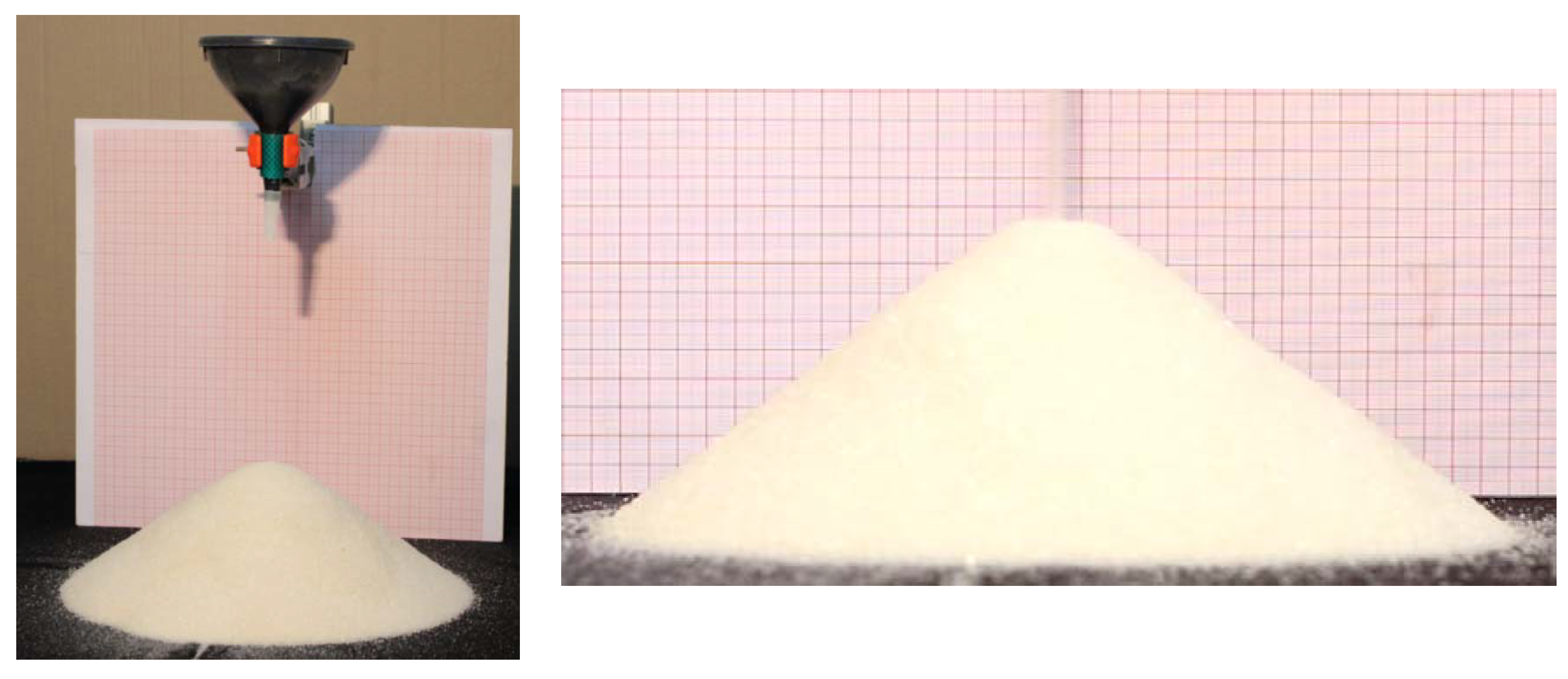
The dynamical behaviour of falling granular matter such as sand is studied (here, granulated sugar). As shown in Figure 1, it is assumed that the granular matter grows under a flow of sand $Q\left(t\right)$ and that the base of the cone created by the accumulation of matter can also grow with time. The experimental apparatus used to create the heap and to measure its height is also described in Figure 1. The sand falls from a conic tank and the height is measured using a webcam.

The time evolution of the sand heap top denoted as $h\left(t\right)$ is represented by Figure 2. The shape of the curve is similar to those represented in [7,8]. In order to show that this system has a power law-type long memory behaviour, the function

$$log\left[h\left(\log \left(t\right)\right)\right]\underset{\mathrm{for}\mathrm{large}t}{~}{K}_0+\nu log\left(t\right)K_0\in ℝ$$

(21)

is represented in Figure 3. For a large time duration, this figure shows that the curve behaves as a straight line:

$$K_0+\nu log\left(t\right)$$

(22)

thus highlighting that the considered system exhibits a power law-type behaviour. Indeed, if $h\left(\mathrm{t}\right)=k_0{t}^{\nu }$ then $log\left[h\left(\mathrm{t}\right)\right]=log\left(k_0\right)+\nu log\left(t\right)=K_0+\nu log\left(t\right)$. Thus, this system has Property 1 of Definition 1.

3.2. Fractional Modelling of the Sand Pile Growth

As the system exhibits a power law-type behaviour, in a first approach, a fractional model was considered to model the system. The proposed model is defined by the transfer function

$$H\left(s\right)=\frac{K}{s^{\nu }}K\in {ℝ}_{+}^{*},\nu \in ℝ,0<\nu <1.$$

(23)

Parameters $K$ and $\nu$ are obtained through the minimisation of a quadratic criterion on the error between the measure and the model time response. The input of the model is assumed to be a Heaviside function of magnitude 1. The parameters obtained are:

$$K=1.23\nu =0.35.$$

(24)

Figure 4 shows a comparison of the measures and the model time response. This comparison reveals that the fractional model permits an accurate fitting of the measures thanks to a compact model involving only two parameters ($K$ and $\nu$). However, such a modelling approach comes with several drawbacks that are now described.

4. Drawbacks of Fractional Modelling

The drawbacks listed in the sequel hold for the fractional modelling approach done in the previous section and beyond. The fractional model obtained in the previous section is a particular form of the more general model

$$H\left(s\right)=\frac{T\left(s\right)}{R\left(s\right)}$$

(25)

with $T\left(s\right)={{\displaystyle \sum }}_{l=0}^r{t}_l{s}^{{\beta }_l}$ and $R\left(s\right)={{\displaystyle \sum }}_{k=0}^m{r}_k{s}^{{\alpha }_k}$ where $r\in {\mathbb{N}}^{*}$, $m\in {\mathbb{N}}^{*}$, $t_l\in ℝ$, $r_k\in ℝ$, ${\beta }_{l+1}\ge {\beta }_l\ge 0$ and ${\alpha }_{k+1}\ge {\alpha }_k\ge 0$. The first drawback associated to this class of model is linked to its physical interpretation. The time constant distribution interpretation is often invoked [9] but does not reflect the internal behaviour of the modelled system, as for example for the case of the pile of sand. The other interpretations are not more satisfactory.

Drawback 1.

The physical interpretations proposed in the literature are not obtained based on the observation of a given phenomenon but result from purely mathematical discussions [9,10,11,12,13,14,15,16,17]. In the case of incommensurate orders, some interpretations can invalidate the obtained model [18].

The impulse response of the Transfer Function (25), computed with the residue theorem using a Bromwich–Wagner path, can be written as [19]:

$$h\left(t\right)=h_p\left(t\right)+h_d\left(t\right)$$

(26)

with

$$h_p\left(t\right)={{\displaystyle \sum }}_{i=1}^n{a}_i{e}^{t{p}_i}n\in {\mathbb{N}}^{*},a_i\in ℝ,p_i\in {ℝ}_{-},\mathrm{and}{h}_d\left(t\right)={{\displaystyle \int }}_0^{\infty }\mu \left(x\right)e^{-tx}dx.$$

(27)

Function $h_p\left(t\right)$ is produced by the poles of the transfer functions $H\left(s\right)$ (residues of the Cauchy method). As explained in [20], the function $\mu \left(x\right)$ in $h_d\left(t\right)$ is defined by

$$\mu \left(x\right)=\frac{1}{2j\pi }\left[H\left({\left(-x\right)}^{-}\right)-H\left({\left(-x\right)}^{+}\right)\right]=\frac{1}{\pi }\frac{{{\displaystyle \sum }}_{k=1}^m{{\displaystyle \sum }}_{l=0}^r{a}_k{q}_{l}sin\left(\pi \left({\alpha }_k-{\beta }_l\right)\right)x^{{\alpha }_k-{\beta }_l}}{{{\displaystyle \sum }}_{k=0}^m{a}_k^2{x}^{2\alpha k}+{{\displaystyle \sum }}_{0\le k<l<m}2a_k{a}_{l}cos\left(\pi \left({\alpha }_k-{\beta }_l\right)\right)x^{{\alpha }_k-{\beta }_l}}.$$

(28)

The Laplace transform of the function $h_d\left(t\right)$ is given by

$$h_d\left(s\right)={{\displaystyle \int }}_0^{\infty }\frac{\mu \left(z\right)}{s+z}{e}^{-tz}dz.$$

(29)

Such a relation shows that a fractional model exhibits poles distributed from 0 to $-\infty$, thus leading to the following drawback.

Drawback 2.

The memory of a fractional model is infinite and it exhibits infinitely slow and infinitely fast time constants (even if they are attenuated through the function$\mu ()$, they exist), which excludes the possibility of linking the model internal variable to a physical variable.

The infinite memory associated to fractional models can also be given by another interpretation. If an input $u\left(t\right)$ is applied to the submodel of the impulse response $h_d\left(t\right)$, the resulting output $y_d\left(t\right)$ is given by the relation [20,21]:

$$\{\begin{array}{l}\frac{\partial w\left(t,z\right)}{\partial t}=-zw\left(t,z\right)+u\left(t\right)\\ y_d\left(s\right)={{\displaystyle \int }}_0^{\infty }\mu \left(z\right)w\left(t,z\right)dz\end{array}\mathrm{with}z\in {ℝ}^{+},$$

(30)

which is known in the literature as diffusive representation [21]. The inverse spatial Fourier transform denoted by the symbol ${\mathcal{F}}^{-1}$ ($\mathcal{F}$ is for Fourier transform) applied to (30), leads to

$$\{\begin{array}{l}\frac{\partial \varphi \left(t,\zeta \right)}{\partial t}=\frac{{\partial }^2\varphi \left(t,\zeta \right)}{\partial {\zeta }^2}+u\left(t\right)\delta \left(\zeta \right)\\ y_d\left(s\right)={{\displaystyle \int }}_{-\infty }^{\infty }m\left(\zeta \right)\varphi \left(t,\zeta \right)d\zeta \end{array}\mathrm{with}\zeta \in ℝ$$

(31)

and

$$\varphi \left(t,\zeta \right)={\mathcal{F}}^{-1}\left\{w\left(t,4{\pi }^2{z}^2\right)\right\},m\left(\zeta \right)={\mathcal{F}}^{-1}\left\{4{\pi }^2\zeta \mu \left(4{\pi }^2{\zeta }^2\right)\right\}.$$

Relation (31) allows us to claim that a fractional system can be associated to an infinite dimensional system described by a diffusion equation on an infinite domain $\left(\zeta \in ℝ\right)$ [22]. It is this (double) infinite dimension requirement that creates the infinite memory mentioned above.

If Model (23) is used for the sand pile growth modelling, an infinite number of initial conditions is required (i.e., a state of infinite dimension is required). However, it is clear that the initial condition of the sand pile growth can be described using a single variable: the sand pile height $h\left(t\right)$ (a state for this system could be chosen as $h\left(t\right)$, making the sand pile growth model a first-order model).

This can also be illustrated in the thermal domain [23]. A fractional integrator is a solution of the heat equation (linking the thermal heat flux applied to the measured temperature) only if:

-

the temperature measure is done at the point where the heat flux is applied; or

-

an infinite dimension medium is considered.

Other spatial configurations can lead to power law-type behaviours but cannot be written under the form of Model (25) (exponential and hyperbolic functions are involved in the Laplace domain).

If orders ${\beta }_l$ and ${\alpha }_k$ meet a commensurate condition in Relation (25), it can be rewritten as:

$$\{\begin{array}{l}\frac{d^{\nu }x\left(t\right)}{d{t}^{\nu }}=Ax\left(t\right)+Bu\left(t\right)\\ y\left(t\right)=Cx\left(t\right)+Du\left(t\right)\end{array}.$$

(32)

In this representation, an analysis of the units very quickly leads to doubts about the physical character of the coefficients in matrices $A$ and $B$, leading to the following drawback.

Drawback 3.

The parameter units associated to description (parameters inside Matrices A and B) have no physical meaning (e.g.,$se{c}^{-\nu }$for parameters in Matrix A).

Representation (32) is known in the literature as a “fractional state space description”. However, this is an improper designation that results from a generalisation of concepts dedicated to integer systems without inquiring into the notion of state. This analysis is demonstrated in [24], and it leads to the following drawback.

Drawback 4.

Representation (32) is not a state space representation, as the variable x(t) does not have the properties of a state. That is why the terms “pseudo state” and “pseudo-state space description” were introduced [24].

In Representation (32), as in the Transfer Function (25), the fractional differentiation operator $\frac{d^{\nu }}{d{t}^{\nu }}$ is not defined uniquely.

Drawback 5.

There are more than 30 definitions of the operator$\frac{d^{\nu }}{d{t}^{\nu }}$[25].

This multiplicity of definitions leads to developing results by choosing the most convenient definition to obtain them. This is why Caputo’s definition became so popular, as it offers the possibility to take into account the initial conditions without taking into account all the past of the system. If from a mathematical point of view the definitions of Caputo, Riemann-Liouville, or others are in no way problematic, their use for the definition of fractional models is questionable. While fractional models are known to have a long and even infinite memory, the use of Caputo’s derivative would make this memory disappear for a given time moment (initial time). This paradoxical situation led to several analyses that revealed the following drawback.

Drawback 6.

The initial conditions are not well taken into account in Representations (32) and (25) if the Caputo or Riemann–Liouville definitions are used [16,22,26,27].

To solve these initialisation issues (and also the infinite memory issue), it was proposed in [28,29] to use a limited frequency band fractional integration operator in the definition of fractional models. Another consequence of the infinite memory of Model (32), and sometimes in contradiction with some results proposed in the literature, is the poor properties of the considered models.

Drawback 7.

Exact observability cannot be reached as all of the system’s past must be known to predict its future [19].

The analysis proposed in [19] could be extended to the analysis of controllability and flatness as model initialisation has an impact on these properties.

To avoid the multiplicity of definitions and the initial conditions problem, it was concluded in [24] that fractional integration is preferable in the definition of a fractional model and thus that Relation (32) should be rewritten under the form:

$$\{\begin{array}{c}x\left(t\right)=I_{t_0\to -\infty }^{\nu }\left[Ax\left(t\right)+Bu\left(t\right)\right]\\ y\left(t\right)=Cx\left(t\right)+Du\left(t\right)\end{array}$$

(33)

with:

$$I_{t_0\to -\infty }^{\nu }\left[f\left(t\right)\right]=\frac{1}{\mathsf{\Gamma }\left(\nu \right)}{{\displaystyle \int }}_{t_0}^t\frac{f\left(\tau \right)}{{\left(t-\tau \right)}^{1-\nu }}d\tau .$$

(34)

However, such a definition entails another drawback.

Drawback 8.

The fractional integration given by Relation (34) involves a singular kernel [30]; this leads to complications in the solution / simulation of the fractional order differential equations.

Note that some non-singular kernels for modelling power law-type long memory behaviours have been proposed in [29].

In the case of the sand pile, the following section shows that all these drawbacks could have been avoided by using a different modelling approach while capturing accurately the power law behaviour.

5. Another Possible Model

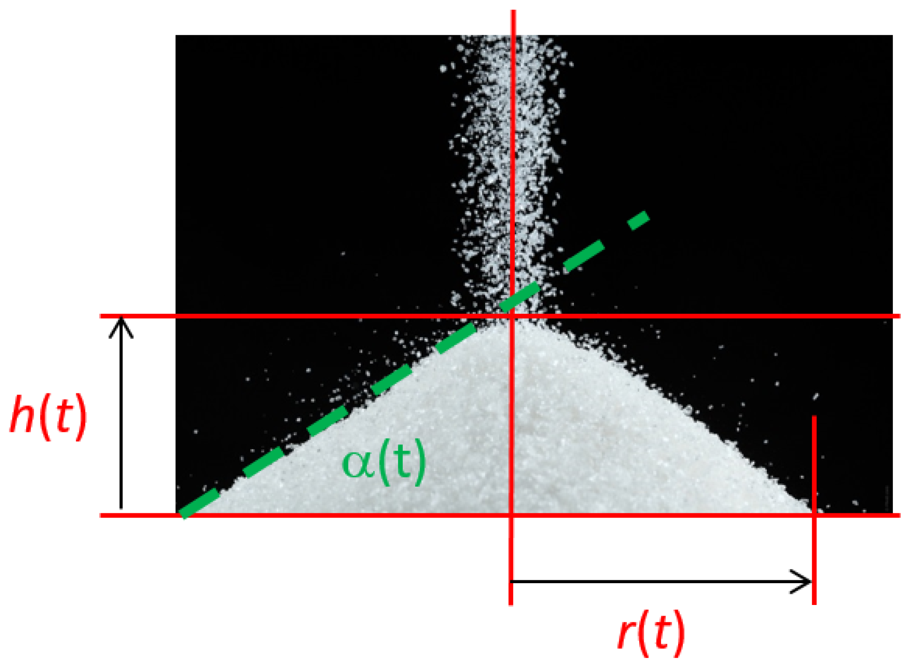
Let $Q\left(t\right)$ be the flow of falling sand. If $V_c\left(t\right)$ denotes the sand heap cone volume with $V_c\left(t\right)=1/3\pi r^{2}h$, according to the notations introduced in Figure 5, the flow $Q\left(t\right)$ generates the volume variation of the cone:

$$\frac{d{V}_c\left(t\right)}{dt}=Q\left(t\right).$$

(35)

As

$$tan\left(\alpha \right)=\frac{h\left(t\right)}{r\left(t\right)}\mathrm{then}{V}_c\left(t\right)=\frac{\pi h{\left(t\right)}^3}{3ta{n}^2\left(\alpha \right)}$$

(36)

and thus, under the hypothesis of a constant angle of repose $\alpha$

$$\frac{d{V}_c\left(t\right)}{dt}=\frac{\pi h{\left(t\right)}^2}{ta{n}^2\left(\alpha \right)}\frac{dh\left(t\right)}{dt}.$$

(37)

Combining Relations (35) and (37), variation in the sand heap height is thus defined by the differential equation:

$$\frac{dh\left(t\right)}{dt}=\frac{ta{n}^2\left(\alpha \right)}{\pi h{\left(t\right)}^2}Q\left(t\right).$$

(38)

For $Q\left(t\right)$ constant, Model (35) can be rewritten as:

$$\frac{dh\left(t\right)}{dt}=\frac{a_0}{h{\left(t\right)}^2}{H}_e\left(t\right),$$

(39)

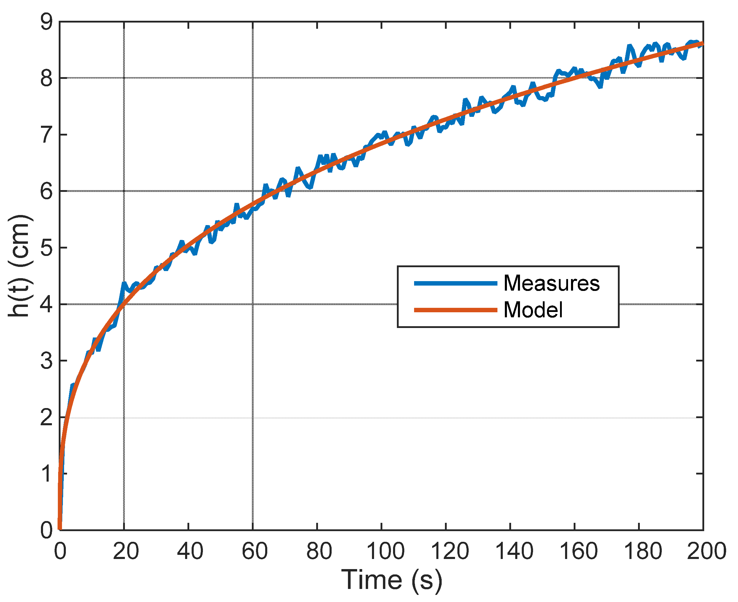
in which $a_0$ is a parameter and $H_e\left(t\right)$ is the Heaviside fonction. With the measures in Figure 2, parameter $a_0$ was computed with an optimisation algorithm aiming at minimising the error between the response of Model (38) and the measures. Parameter $a_0=1.07$ was obtained, and a comparison of the measures with the model response is shown by Figure 6.

Similar to the fractional model, Model (39) also permits an accurate fitting of the system behaviour with a small number of parameters. However, Model (38) resolves most of the drawbacks mentioned in the following paragraph and in particular eliminates any questioning about the infinite space dimension and about initialization of the model.

Let us imagine that the experiment starts with a partially formed sand heap, as if the process had a past. Fractional modelling with Model (23) would impose the knowledge of all the system’s past to restart the experiment, as if knowing the position of all the grains was necessary. However, in practice, this knowledge is not useful. It is not useful to know the position of all the grains of sand; it is only necessary to reconstitute a pile with similar geometric characteristics (angle of repose contained in parameter $a_0$ and heap height $h\left(t\right)$). This is exactly what Model (35) does. Only one state $h\left(t\right)$ and thus its initialisation is required. This example highlights the erroneous conclusions to which fractional modelling can lead. Admittedly, the temporal evolution fitting is very accurate, but the physical interpretation is not possible.

Due to the omnipresence of systems that exhibit power law-type behaviours, it appears important to develop new models that do not exhibit the above problems while being able to capture the corresponding dynamics. Some are proposed in the next section.

6. Beyond Fractional Models

6.1. Some Classes of Non-Linear Models

The previous section showed that models other than fractional models can be used to model power law-type long memory behaviours, in particular non-linear models. This is exactly what the authors did recently for the modelling of the adsorption process [31]. The adsorption process can be likened to the process of the random deposition of discs on a surface, which is denoted random sequential adsorption (RSA) and can be mathematically described as follows.

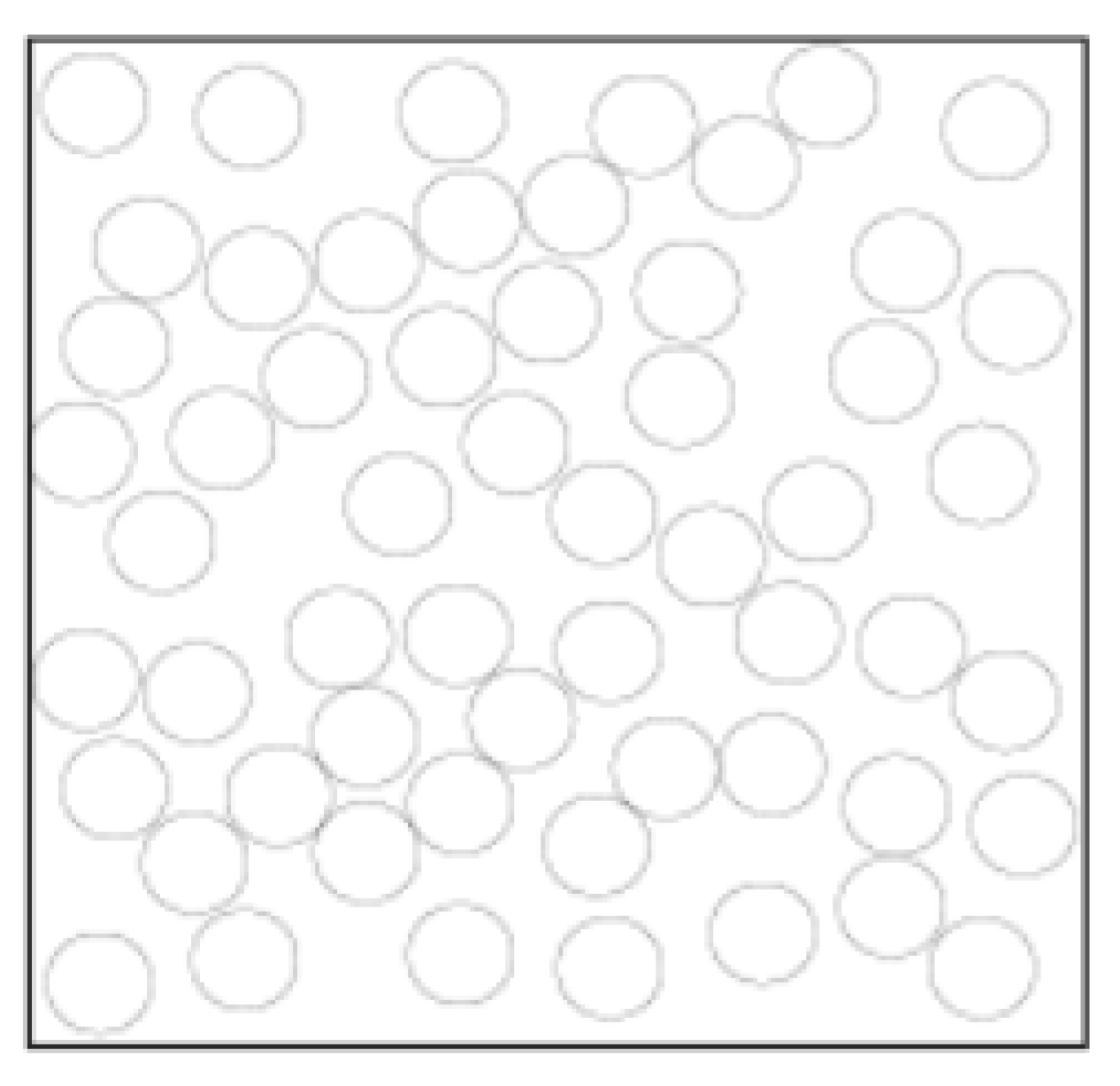
RSA Process: Let $S$ be a square of size $L\times L$, $L\in {ℝ}_{+}^{*}$. Let $R\in {ℝ}_{+}^{*}$ with $R\ll L$ and $t={\left(t_k\right)}_{k\in \mathbb{N}}\in {ℝ}^{\mathbb{N}}$ with $t_0=0$ and such that for all $k\in \mathbb{N}$, $t_{k+1}-t_k=\Delta t\in {ℝ}_{+}^{*}$. At $t=t_0$, the surface is empty. At each time $t_k$, a disk of radius $R$ arrives on the surface $S$ at a randomly chosen location. If the area corresponding to the disk is empty, the disk is placed at the location. If part of the corresponding area is covered by another disk, the disk goes back, and the configuration of $S$ remains unchanged.

An example of the result produced by this process is shown in Figure 7.

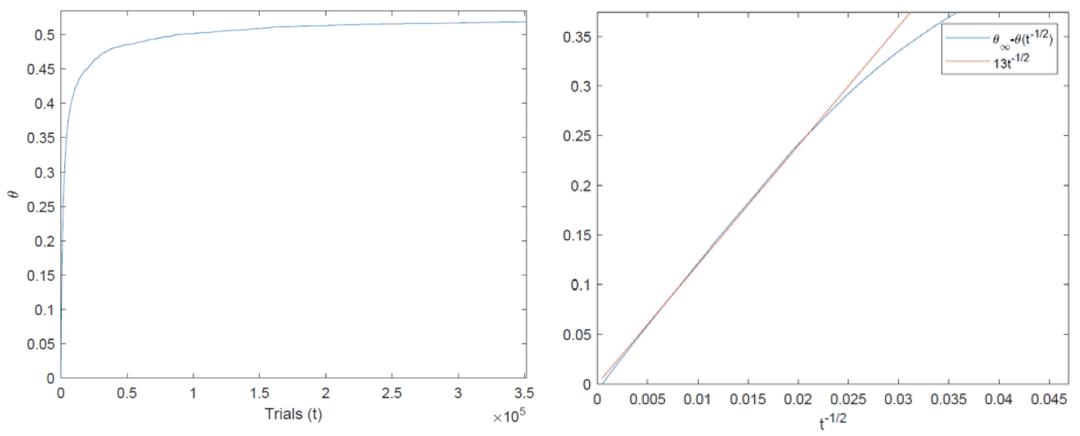
If $\theta \left(t\right)$ denotes the density of the occupied area, it is explained in [32,33], and simulated in [31] that the covered surface can be described by a power law (see Figure 8).

$${\theta }_{\infty }-\theta \left(t\right)\approx t^{-1/2}.$$

(40)

Given the power law behaviour of this process, a fractional model should be effective to describe the kinetic of the density $\theta \left(t\right)$. However, limitations on the ability of this kind of model to capture some properties of the RSA model were highlighted in [31] and are now summarised.

-

With the RSA process (as for the sand pile process), if the flow is stopped, then the surface filling stops. If the flow restarts, the surface filling restarts from the same state. Such behaviour cannot be reproduced with a classical linear fractional model whose output relaxes for a null input.

-

With a fractional modelling approach, an infinite dimensional model is obtained, requiring the entire model past knowledge for a proper initialisation. However, in practice, such knowledge is not required. Initialisation of the RSA process only requires the knowledge of the density $\theta \left(t\right)$ and a uniform distribution of the disks on the surface. Exact knowledge of the position of all the disks on the surface is not necessary, and thus not all the process history is required.

To overcome these limitations, a model of the form

$$\dot{y}\left(t\right)=f\left(y\right)u\left(t\right)$$

(41)

was proposed in [31], in which $u\left(t\right)$ is the flow of disks that hit the surface, $y\left(t\right)=1-\theta \left(t\right)$ denotes the free surface density and

$$f\left(y\right)=\left(b_0+b_{1}y+b_2{y}^2+b_3{y}^3+b_4{y}^4\right)\left[\frac{tanh\left(100\left(y-0.5\right)\right)}{2}-\frac{tanh\left(60\left(y-0.5\right)\right)}{2}\right]+\left(c_0+c_{1}y\right)\frac{tanh\left(60\left(y-0.8\right)\right)+1}{2}.$$

(42)

This model can be viewed as a serious alternative to fractional models as:

-

It permits an accurate fitting of the RSA process kinetic in spite of its power law behaviour;

-

It takes into account some non-linear behaviours in relation to the flow of incoming disks (or particles for the case of a real adsorption process);

-

Its state is only of one dimension, and its initialisation only requires knowledge of the covered density;

-

Its implementation does not require any approximation step.

6.2. Distributed Time Delay Models

Modelling of power law-type long memory behaviours is also possible using distributed time delay systems. This is exactly what is done in [34,35], in which the following class of time delay system is considered.

$$\frac{d}{dt}x\left(t\right)=A_{0}x\left(t\right)+A_1{{\displaystyle \int }}_0^{T_f}\eta \left(\tau \right)x\left(t-\tau \right)d\tau +Bu\left(t\right)$$

(43)

in which

$$\eta \left(t\right)=C_0\left(\frac{{\omega }_l^{\nu }}{\mathsf{\Gamma }\left(\nu \right)}{t}^{\nu -1}{e}^{-{\omega }_{l}t}-\frac{{\omega }_l^{\nu }}{\mathsf{\Gamma }\left(\nu \right)}{t}^{\nu -1}{e}^{-{\omega }_{m}t}+{\omega }_l^{\nu }{\omega }_m^{1-\nu }{e}^{-{\omega }_{m}t}\right)$$

(44)

with

$$C_0=\left|{\left(\frac{1}{{\left(\frac{j}{{\omega }_l}+1\right)}^{\nu }}-{\left(\frac{{\omega }_l}{{\omega }_m}\right)}^{\nu }\frac{1}{{\left(\frac{j}{{\omega }_m}+1\right)}^{\nu }}+{\left(\frac{{\omega }_l}{{\omega }_m}\right)}^{\nu }\frac{1}{\frac{j}{{\omega }_m}+1}\right)}^{-1}\right|.$$

(45)

As shown by Figure 9, the input/output frequency behaviour of such a model exhibits a power law behaviour in a frequency band that can be adjusted using coefficients $A_0$, $A_1$, and $B$.

In comparison with the Fractional Model (32), Model (43) has the following advantages:

-

In Relation (43), the variable $x\left(t\right)$ can be viewed as a real state and a physical meaning can be associated to it;

-

There is no longer any ambiguity in the operator used for the definition of Relation (43) (in Equation (32), Caputo’s, Riemann–Liouville, or another can be chosen);

-

Kernel $\eta \left(t\right)$ in Relation (43) is not singular, unlike the definition of fractional derivative in Equation (32);

-

The memory of Model (43) is of finite length;

-

Initialisation of Model (43) requires knowledge of its state on a finite length and is well defined.

6.3. First Kind Volterra Equations

It must be noted that Fractional Model (32), which is widely used in the literature, is a particular case of a Volterra equation of the first kind. According to [4]—p. 46 (if the fractional integral of order $\nu$ of each component of vector $x\left(t\right)$ exists) and after first-order integration of both sides of the first equation in Relation (32), the following equations can be obtained:

$${{\displaystyle \int }}_0^t{\eta }^{1-\nu }\left(t-\tau \right)x\left(\tau \right)d\tau ={{\displaystyle \int }}_0^t\left[Ax\left(\tau \right)+Bu\left(\tau \right)\right]d\tau$$

(46)

where the kernel in Relation (46) is ${\eta }^{1-\nu }\left(t\right)=t^{-\nu }/\mathsf{\Gamma }\left(1-\nu \right)$ and multiplies each component of vector $x\left(t\right)$. Thus, Representation (32) can be rewritten under the form of a Volterra equation of the first kind,

$${{\displaystyle \int }}_0^t\left(\frac{t^{-\nu }}{\mathsf{\Gamma }\left(1-\nu \right)}{I}_n-A\right)x\left(\tau \right)d\tau =v\left(t\right)\mathrm{with}v\left(t\right)={{\displaystyle \int }}_0^{t}Bu\left(\tau \right)d\tau ,y\left(t\right)=Cx\left(t\right),$$

(47)

where $I_n$ denotes an identity matrix with the same dimension as vector $x\left(t\right)$. Relation (47) demonstrates that a pseudo-state space description is a particular case of a Volterra equation of the first kind, as the kernel in Relation (32) has a fixed structure. Using a Volterra equation, the following class of model can be proposed

$${{\displaystyle \int }}_0^t\eta \left(t-\tau \right)x\left(\tau \right)d\tau =v\left(t\right)\mathrm{with}v\left(t\right)={{\displaystyle \int }}_0^{t}u\left(\tau \right)d\tau ,y\left(t\right)=x\left(t\right)$$

(48)

that generalises the pseudo-state space description (32) in two ways:

• Adapting the kernel $\eta \left(t\right)$ in Relation (48) (see also [29], it is possible to produce, with the same kind of equation, power law behaviours of various types (denoted explicit, implicit), but also many other long memory behaviours;
• In Relation (48), if $x\left(t\right)\in {ℝ}^n$, $\eta \left(t\right)$ is a matrix of kernels such that $\eta \left(t\right)=\left[{\eta }_{i,j}\left(t\right)\right]$, thus permitting great flexibility in the tuning of Relation (48). The case $\eta \left(t\right)=diag\left[{\eta }_i\left(t\right)\right]$ comes closer to the non-commensurate fractional pseudo-state space representation case, but it should be remembered that physical interpretations invalidate this kind of model [18].

Description (48) has another important advantage. Model memory can be limited by introducing a parameter $T_f$ in the integral bounds such that:

$${{\displaystyle \int }}_{t-T_f}^t{\eta }^{\nu }\left(t-\tau \right)x\left(\tau \right)d\tau =v\left(t\right).$$

(49)

Using the change of variable $\xi <t-\tau$, Relation (48) becomes:

$${{\displaystyle \int }}_0^{T_f}{\eta }^{\nu }\left(\xi \right)x\left(t-\xi \right)d\xi =v\left(t\right)\mathrm{with}v\left(t\right)={{\displaystyle \int }}_0^{t}u\left(\tau \right)d\tau ,y\left(t\right)=x\left(t\right).$$

(50)

Relation (50) is close to Relation (43) and explicitly shows that knowledge of the model state $x\left(t\right)$ is required only on $\left[0,T_f\right]$ to compute its future.

7. Conclusions

This paper started from an illustrative example: sand pile growth under the effect of falling sand in the upper part of the heap. Using a simple experiment, it was shown that the pile growth exhibits a power law-type long memory behaviour. As fractional models also exhibit power law-type behaviours, they can be used to capture the input–output behaviour of such a system. However, several drawbacks are associated to this modelling, and were reviewed here. It is shown that a simple non-linear model permits a physical modelling of the considered system, thereby removing all the mentioned drawbacks. This leads to two conclusions:

-

Even if fractional models permit an accurate fitting of power law-type input–output behaviours, they can give birth to disconnected issues of the system considered (initialisation, dimension, interpretations, …)

-

simpler more physical models can be obtained if we try to understand the physical origin of the behaviour.

This is what the authors did to model adsorption phenomena [31]. Yet again, a non-linear model proved to be more suitable than a fractional model for such a modelling problem. However, it is also shown in the rest of the present paper that other models such as distributed time delay models, or a Volterra equation of the first kind, also have the ability to produce power law behaviour without the drawbacks associated to fractional models.

References

- Miller, K.S.; Ross, B. An Introduction to the Fractional Calculus and Fractional Differential Equations; John Wiley & Sons: New York, NY, USA, 1993. [Google Scholar]
- Oldham, K.B.; Spanier, J. The Fractional Calculus; Theory and Applications of Differentiation and Integration to Arbitrary Order (Mathematics in Science and Engineering, V); Academic Press: Cambridge, MA, USA, 1974. [Google Scholar]
- Podlubny, I. Fractional Differential Equations. Mathematics in Sciences and Engineering; Academic Press: Cambridge, MA, USA, 1999. [Google Scholar]
- Samko, S.G.; Kilbas, A.A.; Marichev, O.I. Fractional Integrals and Derivatives: Theory and Applications; Gordon and Breach Science Publishers: London, UK, 1993. [Google Scholar]
- Bagley, R.L.; Calico, R.A. Fractional order state equations for the control of viscoelastically damped structures. J. Guid. Control Dyn. 1991, 14, 304–311. [Google Scholar] [CrossRef]
- Oppenheim, A.V.; Alan SWillsky, A.S.; Hamid, S. Signals and Systems, Pearson New International Edition; Pearson Education Limited: Harlow, UK, 1996. [Google Scholar]
- Mandal, S.; Khakhar, D. Granular surface flow on an asymmetric conical heap. J. Fluid Mech. 2019, 865, 41–59. [Google Scholar] [CrossRef]
- Pacheco-Vazquez, F.; Moreau, F.; Vandewalle, N.; Dorbolo, S. Sculpting sandcastles grain by grain: Self-assembled sand towers. Phys. Rev. E 2012, 86, 051303. [Google Scholar] [CrossRef] [PubMed] [Green Version]
- Oustaloup, A. Diversity and Non-Integer Differentiation for System Dynamics; Wiley: Hoboken, NJ, USA, 2014. [Google Scholar]
- Ben Adda, F. Geometric interpretation of the fractional derivative. J. Fract. Calc. 1997, 11, 21–52. [Google Scholar]
- Podlubny, I. Geometric and physical interpretation of fractional integration and fractional differentiation. J. Fract. Calc. Appl. Anal. 2002, 5, 357–366. [Google Scholar]
- Gorenflo, R. Afterthoughts on interpretation of fractional derivatives and integrals. In Transform Methods and Special Functions, Varna’96, Institute of Mathematics and Informatics; Rusev, P., Dimovski, I., Kiryakova, V., Eds.; Bulgarian Academy of Sciences: Bulgarian, Sofia, 1998. [Google Scholar]
- Mainardi, F. Considerations on fractional calculus: Interpretations and applications. In Transform Methods and Special Functions, Varna’96, Institute of Mathematics and Informatics; Rusev, P., Dimovski, I., Kiryakova, V., Eds.; Bulgarian Academy of Sciences: Bulgarian, Sofia, 1998. [Google Scholar]
- Nigmatullin, R.R. A fractional integral and its physical interpretation. Theoret. and Math. Physics 1992, 90, 242–251. [Google Scholar] [CrossRef]
- Rutman, R.S. On physical interpretations of fractional integration and differentiation. Theor. Math. Phys. 1995, 105, 393–404. [Google Scholar] [CrossRef]
- Sabatier, J.; Merveillaut, M.; Malti, R.; Oustaloup, A. On a Representation of Fractional Order Systems: Interests for the Initial Condition Problem. In Proceedings of the 3rd IFAC Workshop on “Fractional Differentiation and its Applications” (FDA’08), Ankara, Turkey, 5–7 November 2008. [Google Scholar]
- Tenreiro Machado, J.A. A probabilistic Interpretation of the Fractional-Order differentiation. J. Fract. Calc. Appl. Anal. 2003, 6, 73–80. [Google Scholar]
- Dokoumetzidis, A.; Magin, R.; Macheras, P. A commentary on fractionalization of multi-compartmental models. Pharm. Pharm. 2010, 37, 203–207. [Google Scholar] [CrossRef]
- Sabatier, J.; Farges, C.; Merveillaut, M.; Feneteau, L. On observability and pseudo state estimation of fractional order systems. Eur. J. Control 2012, 18, 260–271. [Google Scholar] [CrossRef]
- Matignon, D. Stability properties for generalized fractional differential systems. ESAIM Proc. 1998, 5, 145–158. [Google Scholar] [CrossRef] [Green Version]
- Montseny, G. Diffusive representation of pseudo-differential time-operators. ESAIM Proc. 1998, 5, 159–175. [Google Scholar] [CrossRef]
- Sabatier, J.; Merveillaut, M.; Malti, R.; Oustaloup, A. How to Impose Physically Coherent Initial Conditions to a Fractional System? Commun. Nonlinear Sci. Numer. Simul. 2010, 15, 1318–1326. [Google Scholar] [CrossRef]
- Sabatier, J.; Nguyen, H.C.; Farges, C.; Deletage, J.Y.; Moreau, X.; Guillemard, F.; Bavoux, B. Fractional models for thermal modeling and temperature estimation of a transistor junction. Adv. Differ. Equ. 2011. [Google Scholar] [CrossRef] [Green Version]
- Sabatier, J.; Farges, C.; Trigeassou, J.C. Fractional systems state space description: Some wrong ideas and proposed solutions. J. Vib. Control 2014, 20, 1076–1084. [Google Scholar] [CrossRef]
- De Oliveira, E.C.; Tenreiro Machado, J.A. A Review of Definitions for Fractional Derivatives and Integral. Math. Probl. Eng. 2019, 2014, 238459. [Google Scholar] [CrossRef] [Green Version]
- Sabatier, J.; Farges, C. Comments on the description and initialization of fractional partial differential equations using Riemann-Liouville’s and Caputo’s definitions. J. Comput. Appl. Math. 2018, 339, 30–39. [Google Scholar] [CrossRef]
- Ortigueira, M.D.; Coito, F.J. Initial Conditions: What Are We Talking about? In Proceedings of the Third IFAC Workshop on Fractional Differentiation, Ankara, Turkey, 5–7 November 2008. [Google Scholar]
- Sabatier, J.; Rodriguez Cadavid, S.; Farges, C. Advantages of limited frequency band fractional integration operator in fractional models definition. In Proceedings of the Conference on Control, Decision and Information Technologies (CoDIT 2019), Paris, France, 23–26 April 2019. [Google Scholar]
- Sabatier, J. Non-Singular Kernels for Modelling Power Law Type Long Memory Behaviours and Beyond. Cybernetics 2020. accepted. [Google Scholar]
- Caputo, M.; Fabrizio, M. A new definition of fractional derivative without singular kernel. Prog. Fract. Differ. Appl. 2015, 1, 73–85. [Google Scholar]
- Tartaglione, V.; Farges, C.; Sabatier, J. Dynamical Modelling of Random Sequential Adsorption. In Proceedings of the European Control Conference ECC 2020, St-Petersburg, Russia, 12–15 May 2020. [Google Scholar]
- Feder, J.; Giaever, I. Adsorption of ferritin. J. Colloid Interface Sci. 1980, 78, 144–154. [Google Scholar] [CrossRef]
- Viot, P.; Tarjus, G.; Ricci, S.; Talbot, J. Random sequential adsorption of anisotropic particles. I. jamming limit and asymptotic behavior. J. Chem. Phys. 1992, 97, 5212–5218. [Google Scholar] [CrossRef] [Green Version]
- Sabatier, J. Distributed time delay systems for power law long memory behaviors modelling. In Proceedings of the 58th Conference on Decision and Control (CDC 2019), Nice, France, 11–13 December 2019. [Google Scholar]
- Sabatier, J. Power Law Type Long Memory Behaviors Modeled with Distributed Time Delay Systems. Fract. Fractals 2020, 4, 1. [Google Scholar] [CrossRef] [Green Version]
Figure 1.
Illustration of sand pile growth (right) and description of the apparatus used to measure the heap height (left).
Figure 2.
Heap top variation.
Figure 3.
Function
Figure 4.
Comparison of the measures and the model response.
Figure 5.
Notations for the characterisation of the sand heap growth.
Figure 6.
Comparison of the measures with the Model (35) response.
Figure 7.
A possible result for the random sequential adsorption (RSA) process.
Figure 8.
Density of occupied area as a function of trials (left) and highlighting of the power law behaviour of for large values of t (right).
Figure 9.
Gain (left) and phase (right) diagrams of for various values of where corner frequencies , , and depend on parameters , , and [34].
© 2020 by the authors. Licensee MDPI, Basel, Switzerland. This article is an open access article distributed under the terms and conditions of the Creative Commons Attribution (CC BY) license (http://creativecommons.org/licenses/by/4.0/).
Share and Cite
MDPI and ACS Style
Sabatier, J.; Farges, C.; Tartaglione, V. Some Alternative Solutions to Fractional Models for Modelling Power Law Type Long Memory Behaviours. Mathematics 2020, 8, 196. https://0-doi-org.brum.beds.ac.uk/10.3390/math8020196
AMA Style
Sabatier J, Farges C, Tartaglione V. Some Alternative Solutions to Fractional Models for Modelling Power Law Type Long Memory Behaviours. Mathematics. 2020; 8(2):196. https://0-doi-org.brum.beds.ac.uk/10.3390/math8020196
Chicago/Turabian StyleSabatier, Jocelyn, Christophe Farges, and Vincent Tartaglione. 2020. "Some Alternative Solutions to Fractional Models for Modelling Power Law Type Long Memory Behaviours" Mathematics 8, no. 2: 196. https://0-doi-org.brum.beds.ac.uk/10.3390/math8020196
Note that from the first issue of 2016, this journal uses article numbers instead of page numbers. See further details here.