Robust Linear Trend Test for Low-Coverage Next-Generation Sequence Data Controlling for Covariates

Abstract

Low-coverage next-generation sequencing experiments assisted by statistical methods are popular in a genetic association study. Next-generation sequencing experiments produce genotype data that include allele read counts and read depths. For low sequencing depths, the genotypes tend to be highly uncertain; therefore, the uncertain genotypes are usually removed or imputed before performing a statistical analysis. It may result in the inflated type I error rate and in a loss of statistical power. In this paper, we propose a mixture-based penalized score association test adjusting for non-genetic covariates. The proposed score test statistic is based on a sandwich variance estimator so that it is robust under the model misspecification between the covariates and the latent genotypes. The proposed method takes advantage of not requiring either external imputation or elimination of uncertain genotypes. The results of our simulation study show that the type I error rates are well controlled and the proposed association test have reasonable statistical power. As an illustration, we apply our statistic to pharmacogenomics data for drug responsiveness among 400 epilepsy patients.

1. Introduction

Genome-wide association study (GWAS) is a powerful tool for screening a high-dimensional genome data set and selecting candidate genetic variants such as single nucleotide polymorphisms (SNPs) in genetic association studies. Next-generation sequencing (NGS) technology is widely used to produce a large amount of genetic information in a fast way. In the past decade, there have been numerous studies using NGS data such as rare variants association study [1,2], pharmacogenomics [3,4], machine learning and deep learning applications [5,6], and big data analysis [7,8]. Many NGS experiments are based on low-coverage sequencing with a large sized sample since there is a trade-off between sample size and sequencing depth in the NGS experiments [9,10]. For the low-coverage NGS data, a high uncertainty of the inferred genotypes is common; however, it causes biased and unreliable results on genetic association analyses. In genetic research based on NGS data, therefore, it is important to obtain accurate genotypes to perform an association analysis.

A number of researchers have worked on the effects of genotype misclassification in genetic association studies. There are two types of genotype misclassifications: differential and non-differential misclassifications, determined by whether the misclassification mechanism differs in the case and control groups or not. In summary, non-differential misclassifications result in a loss of statistical power and differential misclassifications distort type I error rates in a genetic case-control association study [11,12,13,14].

While there have been many research on improving the accuracy of genotypes such as the joint genotype calling algorithms across all samples were suggested to increase the accuracy of genotype calls [15,16,17], several researchers have tried to develop new association statistics accounting for the genotype errors. Their approaches are based on the raw measurements rather than inferred genotypes. In statistical genetics literature, Kim et al. [18] extended a chi-squared test of independence and developed a mixture likelihood based association test using the continuous measurements for copy number polymorphisms. Barnes et al. [19] proposed a mixture model linear trend test for the continuous copy number measurements. In NGS experiments, a likelihood ratio test based on allele read counts of pooled samples was proposed to test independence of genetic variants with a binary phenotype [20]. Gordon et al. [21] proposed a likelihood ratio test of the binomial mixture model of allele read counts with known error parameters. Kim et al. [13,22] proposed an extended version of Cochran–Armitage (CA) trend test and a multi-variant linear trend test for next-generation sequences data by using binomial mixture models. For a case-parent trio design, the binomial mixture model was applied to develop extended transmission disequilibrium tests (TDTs) based on read counts and read depths and to provide power analysis and sample size formulas [23]. All these approaches do not require genotype calls that can be highly uncertain when the read depth or coverage is low. However, none of these previous research has addressed how to include covariates in their mixture-based association studies.

When the covariates are independent of the latent genotypes, the extension of the mixture model based association tests is straightforward. However, if the latent genotype variable is associated with other covariates, then a likelihood based approach requires a model specification between the genotype variable and the other covariates as opposed to the previous research [16,17,18,19,20,21,22,23]. To our knowledge, this is the first study that investigates a genetic case-control association test controlling for covariates in low-coverage NGS experiments. Since we do not know the true model, we apply a sandwich variance estimator to develop a robust genetic association test statistic.

2. Materials and Methods

2.1. Mixture Model Accounting for Covariates

Let $\mathbf{w}$ be a covariate vector. Let y be a random variable indicating the case-control status of an individual such that $y=1$ if a subject is in the case group and $y=0$, otherwise. Let $\mathbf{z}=(z_0,z_1,z_2)$ denote an unobservable latent genotype vector, where ${\sum }_{g=0}^2{z}_g=1$ and $z_g=1$ if and only if the genotype is equal to g. Let x and v denote the minor allele read count and the read depth, respectively. The probability function is given by

$$\begin{array}{cc}p(y,x,v,\mathbf{w})\hfill & =\sum _{\mathbf{z}}p(y,x,v,\mathbf{w},\mathbf{z})\hfill \\ & =\sum _{\mathbf{z}}p\left(x\right|v,\mathbf{w},\mathbf{z},y)p\left(y\right|v,\mathbf{w},\mathbf{z})p\left(\mathbf{z}\right|\mathbf{w},v)p(\mathbf{w},v)\hfill \\ & =p(\mathbf{w},v)\sum _{\mathbf{z}}p\left(x\right|v,\mathbf{z},y)p\left(y\right|\mathbf{z},\mathbf{w})p\left(\mathbf{z}\right|\mathbf{w}).\hfill \end{array}$$

(1)

If the probability function of the read count x does not depend on the phenotype y, that is, $p\left(x\right|v,\mathbf{z},y)=p(x|v,\mathbf{z})$, then it is called a non-differential error model. We apply a binary logit model to the case-control phenotype response variable y that is the same model for Cochran–Armitage trend test when perfect genotypes are available:

$$\begin{array}{ccc}\hfill p\left(y\right|\mathbf{z},\mathbf{w})& =& \frac{e^{y(\beta {\mathbf{s}}^T\mathbf{z}+{\beta }_w^T\mathbf{w})}}{1+e^{{\beta }_0+\beta {\mathbf{s}}^T\mathbf{z}+{\beta }_w^T\mathbf{w}}}.\hfill \end{array}$$

(2)

We assume a binomial error model to the allele read counts as in previous research [13,16,20,21,23]:

$$\begin{array}{ccc}p\left(x\right|v,\mathbf{z},y)\hfill & =& \left(\genfrac{}{}{0pt}{}{v}{x}\right){\left({\mathbf{u}}_{ϵ}^T\mathbf{z}\right)}^x{\left(1-{\mathbf{u}}_{ϵ}^T\mathbf{z}\right)}^{v-x},\hfill \end{array}$$

(3)

where ${\mathbf{u}}_{ϵ}={(ϵ,1/2,1-ϵ)}^T$. For a differential error model, we can use ${\mathbf{u}}_{ϵ}=y{({ϵ}_1,1/2,1-{ϵ}_1)}^T+(1-y){({ϵ}_0,1/2,1-{ϵ}_0)}^T$. When perfect genotypes are available, we do not need the conditional probability of the genotype $\mathbf{z}$ given covariates $\mathbf{w}$ to perform genetic association tests since the logistic regression model is a conditional model given the genotypes and covariates. In this work, we assume a multinomial logit model for the latent genotype given the covariates as follows:

$$\begin{array}{ccc}p\left(\mathbf{z}\right|\mathbf{w})\hfill & =& \frac{{\sum }_{g=0}^2{z}_g{e}^{{\gamma }_g^T\mathbf{w}}}{{\sum }_{m=0}^2{e}^{{\gamma }_m^T\mathbf{w}}},\hfill \end{array}$$

(4)

where ${\gamma }_0={(0,0,0)}^T$ to remove over-parametrization. Other statistical models without the assumptions of a multinomial logit model may also be used for the relationship between covariates and latent genotypes, where we do not know the true model.

The likelihood function L and the log-likelihood function ℓ are written as

$$\begin{array}{cc}L\hfill & =\prod _{k=1}^N\left[\sum _{{\mathbf{z}}_k}p\left(y_k\right|{\mathbf{z}}_k,{\mathbf{w}}_k)p\left(x_k\right|v_k,{\mathbf{z}}_k,y_k)p\left({\mathbf{z}}_k\right|{\mathbf{w}}_k)p({\mathbf{w}}_k,v_k)\right]\hfill \\ & =\prod _{k=1}^N\sum _{i=0}^2\left\{\left(\frac{e^{y_k(\beta s_i+{\beta }_w^T{\mathbf{w}}_k)}}{1+e^{\beta s_i+{\beta }_w^T{\mathbf{w}}_k}}\right)\left(\left(\genfrac{}{}{0pt}{}{v_k}{x_k}\right){\left(u_{ϵi}\right)}^{x_k}{\left(1-u_{ϵi}\right)}^{v_k-x_k}\right)\left(\frac{e^{{\gamma }_i^T{\mathbf{w}}_k}}{{\sum }_{m=0}^2{e}^{{\gamma }_m^T{\mathbf{w}}_k}}\right)p({\mathbf{w}}_k,v_k)\right\},\hfill \end{array}$$

(5)

$$\begin{array}{ccc}\ell \hfill & =& \sum _{k=1}^{N}log\left[\sum _{i=0}^2\left\{\left(\frac{e^{y_k(\beta s_i+{\beta }_w^T{\mathbf{w}}_k)}}{1+e^{\beta s_i+{\beta }_w^T{\mathbf{w}}_k}}\right)\left({\left(u_{ϵi}\right)}^{x_k}{\left(1-u_{ϵi}\right)}^{v_k-x_k}\right)\left(\frac{e^{{\gamma }_i^T{\mathbf{w}}_k}}{{\sum }_{m=0}^2{e}^{{\gamma }_m^T{\mathbf{w}}_k}}\right)\right\}\right]\hfill \\ & & +\sum _{k=1}^{N}log\left(\genfrac{}{}{0pt}{}{v_k}{x_k}\right)p({\mathbf{w}}_k,v_k).\hfill \end{array}$$

(6)

The error parameter $ϵ$ is commonly small and hence the estimate of $ϵ$ is often equal to zero. The zero estimate of the error parameter results in a divergent information matrix. It prevents us from calculating Rao’s score test statistic. In order to overcome this issue, we include a beta density penalty term to prevent from zero estimate of the error parameter. The penalized log-likelihood function is given by

$$\begin{array}{ccc}{\ell }_p\hfill & =& \ell +Clog\left[{ϵ}^{a_{ϵ}}{(1-ϵ)}^{b_{ϵ}}\right].\hfill \end{array}$$

(7)

During this work, we choose $C=1$ as in [24,25]. The penalized complete-data likelihood function is given by

$$\begin{array}{ccc}{L}_C\hfill & =& \prod _{k=1}^N\prod _{i=0}^2{\left[\frac{e^{y_k(\beta s_i+{\beta }_w^T{\mathbf{w}}_k)}}{1+e^{\beta s_i+{\beta }_w^T{\mathbf{w}}_k}}\times \left(\genfrac{}{}{0pt}{}{v_k}{x_k}\right){\left(u_{ϵi}\right)}^{x_k}{(1-u_{ϵi})}^{v_k-x_k}{ϵ}^{\frac{a_{ϵ}}{N}}{(1-ϵ)}^{\frac{b_{ϵ}}{N}}\times \frac{e^{{\gamma }_i^T{\mathbf{w}}_k}}{{\sum }_{m=0}^2{e}^{{\gamma }_m^T{\mathbf{w}}_k}}\right]}^{z_{ik}}\hfill \end{array}$$

(8)

The complete data log-likelihood function is written as

$$\begin{array}{ccc}{\ell }_C\hfill & =& \sum _{k=1}^N\sum _{i=0}^2{z}_{ik}\left[y_k(\beta s_i+{\beta }_w^T{\mathbf{w}}_k)-log\left(1+e^{\beta s_i+{\beta }_w^T{\mathbf{w}}_k}\right)\right]\hfill \\ & & +\sum _{k=1}^N\sum _{i=0}^2{z}_{ik}\left[x_{k}log\left(u_{ϵi}\right)+(v_k-x_k)log(1-u_{ϵi})\right]+a_{ϵ}logϵ+b_{ϵ}log(1-ϵ)\hfill \\ & & +\sum _{k=1}^N\sum _{i=0}^2{z}_{ik}\left[{\gamma }_i^T{\mathbf{w}}_k-log\left(\sum _{m=0}^2{e}^{{\gamma }_m^T{\mathbf{w}}_k}\right)\right].\hfill \end{array}$$

(9)

2.2. Derivation of EM Algorithm under $H_0$

We apply the Expectation–Maximization (EM) algorithm [26] to estimate the parameters in our mixture model. Given data and the $\left(r\right)$-th step estimated parameters, the $(r+1)$-th E-step of the EM algorithm is written as

$$\begin{array}{ccc}{Q}^{(r+1)}\hfill & =& \sum _{k=1}^N\sum _{i=0}^2{\tau }_{ik}^{\left(r\right)}\left[y_k(\beta s_i+{\beta }_w^T{\mathbf{w}}_k)-log\left(1+e^{\beta s_i+{\beta }_w^T{\mathbf{w}}_k}\right)\right]\hfill \\ & & +\sum _{k=1}^N\sum _{i=0}^2{\tau }_{ik}^{\left(r\right)}\left[x_{k}log\left(u_{ϵi}\right)+(v_k-x_k)log(1-u_{ϵi})\right]+a_{ϵ}logϵ+b_{ϵ}log(1-ϵ)\hfill \\ & & +\sum _{k=1}^N\sum _{i=0}^2{\tau }_{ik}^{\left(r\right)}\left[{\gamma }_i^T{\mathbf{w}}_k-log\left(\sum _{m=0}^2{e}^{{\gamma }_m^T{\mathbf{w}}_k}\right)\right],\hfill \end{array}$$

(10)

where

$$\begin{array}{cc}{\tau }_{ik}^{\left(r\right)}\hfill & =\frac{\left(\frac{e^{y_k({\beta }^{\left(r\right)}{s}_i+{\beta }_w^{\left(r\right)T}{\mathbf{w}}_k)}}{1+e^{{\beta }^{\left(r\right)}{s}_i+{\beta }_w^{\left(r\right)T}{\mathbf{w}}_k}}\right)\left({(u_{ϵi}^{\left(r\right)})}^{x_k}{(1-u_{ϵi}^{\left(r\right)})}^{v_k-x_k}\right)\left(\frac{e^{{\gamma }_i^{\left(r\right)T}{\mathbf{w}}_k}}{{\sum }_{m=0}^2{e}^{{\gamma }_m^{\left(r\right)T}{\mathbf{w}}_k}}\right)}{{\sum }_{g=0}^2\left[\left(\frac{e^{y_k({\beta }^{\left(r\right)}{s}_g+{\beta }_w^{\left(r\right)T}{\mathbf{w}}_k)}}{1+e^{{\beta }^{\left(r\right)}{s}_g+{\beta }_w^{\left(r\right)T}{\mathbf{w}}_k}}\right)\left({(u_{ϵg}^{\left(r\right)})}^{x_k}{(1-u_{ϵg}^{\left(r\right)})}^{v_k-x_k}\right)\left(\frac{e^{{\gamma }_g^{\left(r\right)T}{\mathbf{w}}_k}}{{\sum }_{m=0}^2{e}^{{\gamma }_m^{\left(r\right)T}{\mathbf{w}}_k}}\right)\right]}.\end{array}$$

(11)

We note that the posterior probability of subject k belonging to genotype class i depends on the all parameters. In M-step, the $(r+1)$-th estimates of the parameters are obtained by maximizing $Q^{(r+1)}$:

$$\begin{array}{ccc}\frac{\partial Q^{(r+1)}}{\partial \beta }\hfill & =& \sum _{k=1}^N\sum _{i=0}^2{\tau }_{ik}^{\left(r\right)}{s}_i\left(y_k-{\pi }_{ik}\right)=0\hfill \end{array}$$

(12)

$$\begin{array}{ccc}\frac{\partial Q^{(r+1)}}{\partial {\beta }_w}\hfill & =& \sum _{k=1}^N\sum _{i=0}^2{\tau }_{ik}^{\left(r\right)}{\mathbf{w}}_k\left(y_k-{\pi }_{ik}\right)=0\hfill \end{array}$$

(13)

$$\begin{array}{ccc}\frac{\partial Q^{(r+1)}}{\partial ϵ}\hfill & =& \sum _{k=1}^N\left[{\tau }_{0k}^{\left(r\right)}\left(\frac{x_k}{ϵ}-\frac{v_k-x_k}{1-ϵ}\right)+{\tau }_{2k}^{\left(r\right)}\left(\frac{v_k-x_k}{ϵ}-\frac{x_k}{1-ϵ}\right)\right]+\frac{a_{ϵ}}{ϵ}-\frac{b_{ϵ}}{1-ϵ}=0\hfill \end{array}$$

(14)

$$\begin{array}{ccc}\frac{\partial Q^{(r+1)}}{\partial {\gamma }_i}\hfill & =& \sum _{k=1}^N{\mathbf{w}}_k\left({\tau }_{ik}^{\left(r\right)}-p_{ik}\right)=0,\hfill \end{array}$$

(15)

where we use notations ${\pi }_{ik}={\pi }_{ik}(\beta ,{\beta }_w)=\frac{e^{\beta s_i+{\beta }_w^T{\mathbf{w}}_k}}{1+e^{\beta s_i+{\beta }_w^T{\mathbf{w}}_k}}$ and $p_{ik}=p_{ik}({\gamma }_1,{\gamma }_2)=\frac{e^{{\gamma }_i^T{\mathbf{w}}_k}}{{\sum }_{m=0}^2{e}^{{\gamma }_m^T{\mathbf{w}}_k}}$ for simplicity. From Equation (14), we derive a closed form iteration formula to update the allele read error parameter $ϵ$:

$$\begin{array}{ccc}{ϵ}^{(r+1)}\hfill & =& \frac{{\sum }_{k=1}^N\left[{\tau }_{0k}^{\left(r\right)}{x}_k+{\tau }_{2k}^{\left(r\right)}(v_k-x_k)\right]+a_{ϵ}}{{\sum }_{k=1}^N\left[({\tau }_{0k}^{\left(r\right)}+{\tau }_{2k}^{\left(r\right)})v_k\right]+a_{ϵ}+b_{ϵ}}.\hfill \end{array}$$

(16)

There is no closed form iteration formulas to update other parameters $\beta ,{\beta }_w,{\gamma }_i$. The M-step for $\beta ,{\beta }_w$, and $\gamma$ can be obtained by the Newton–Raphson method. The Hessian matrix of $Q^{(r+1)}$ is given by

$$\begin{array}{ccc}\frac{{\partial }^2{Q}^{(r+1)}}{\partial {\beta }^2}\hfill & =& -\sum _{k=1}^N\sum _{i=0}^2{\tau }_{ik}^{\left(r\right)}{s}_i^2\left[{\pi }_{ik}(1-{\pi }_{ik})\right]\hfill \end{array}$$

(17)

$$\begin{array}{ccc}\frac{{\partial }^2{Q}^{(r+1)}}{\partial \beta \partial {\beta }_w}\hfill & =& -\sum _{k=1}^N\sum _{i=0}^2{\tau }_{ik}^{\left(r\right)}{s}_i{\mathbf{w}}_k\left[{\pi }_{ik}(1-{\pi }_{ik})\right]\hfill \end{array}$$

(18)

$$\begin{array}{ccc}\frac{{\partial }^2{Q}^{(r+1)}}{\partial {\beta }_w\partial {\beta }_w^T}\hfill & =& -\sum _{k=1}^N\sum _{i=0}^2{\tau }_{ik}^{\left(r\right)}{\mathbf{w}}_k{\mathbf{w}}_k^T\left[{\pi }_{ik}(1-{\pi }_{ik})\right]\hfill \end{array}$$

(19)

$$\begin{array}{ccc}\frac{{\partial }^2{Q}^{(r+1)}}{\partial {\gamma }_i\partial {\gamma }_i^T}\hfill & =& -\sum _{k=1}^N{\mathbf{w}}_k{\mathbf{w}}_k^T\left[p_{ik}(1-p_{ik})\right]\hfill \end{array}$$

(20)

$$\begin{array}{ccc}\frac{{\partial }^2{Q}^{(r+1)}}{\partial {\gamma }_i\partial {\gamma }_j^T}\hfill & =& \sum _{k=1}^N{\mathbf{w}}_k{\mathbf{w}}_k^T\left[p_{ik}{p}_{jk}\right]\hfill \end{array}$$

(21)

$$\begin{array}{ccc}\frac{{\partial }^2{Q}^{(r+1)}}{\partial {\gamma }_i\partial {\beta }_w^T}\hfill & =& \frac{{\partial }^2{Q}^{(r+1)}}{\partial {\gamma }_i\partial \beta }=0\hfill \end{array}$$

(22)

Let $M=\mathrm{diag}\left({\sum }_{i=0}^2{\tau }_{ik}{\pi }_{ik}(1-{\pi }_{ik})\right)$ be an $N\times N$ diagonal matrix. Let $W=\left(w_{ik}\right)$ be the $N\times p$ matrix of covariates. Let $\mu$ be an $N\times 1$ vector of ${\mu }_k={\sum }_{ik}{\tau }_{ik}{\pi }_{ik}$ and Y be an $N\times 1$ vector of $y_k$. Initially, we set ${\beta }^{\left[0\right]}={\beta }^{\left(r\right)}$ and update the parameter estimate by

$$\begin{array}{ccc}{\beta }^{[t+1]}\hfill & =& {\beta }^{\left[t\right]}+{\left(W^{T}MW\right)}^{-1}{W}^T(Y-\mu ).\hfill \end{array}$$

(23)

Let $D_{11}=\mathrm{diag}\left(p_{1k}(1-p_{1k})\right),D_{12}=D_{21}=-\mathrm{diag}\left(p_{1k}{p}_{2k}\right)$, and $D_{22}=\mathrm{diag}\left(p_{2k}(1-p_{2k})\right)$. Let ${\tau }_i=\left({\tau }_{ik}\right)$ be the $N\times 1$ vector and $p_i=\left(p_{ik}\right)$ be the $N\times 1$ vector. Initially, set ${\gamma }_i^{\left[0\right]}={\gamma }_i^{\left(r\right)}$ and update the parameters ${\gamma }_i$ by

$$\begin{array}{ccc}\left(\begin{array}{c}{\gamma }_1^{[t+1]}\\ {\gamma }_2^{[t+1]}\end{array}\right)\hfill & =& \left(\begin{array}{c}{\gamma }_1^{\left[t\right]}\\ {\gamma }_2^{\left[t\right]}\end{array}\right)+{\left(\begin{array}{cc}{W}^T{D}_{11}W& W^T{D}_{12}W\\ W^T{D}_{21}W& W^T{D}_{22}W\end{array}\right)}^{-1}\left(\begin{array}{c}{W}^T({\tau }_1-p_1)\\ W^T({\tau }_2-p_2)\end{array}\right).\hfill \end{array}$$

(24)

In order to obtain ${\beta }_w^{(r+1)}$ and ${\gamma }_i^{(r+1)}$, we stop the iterations in the M-step for $\beta$ and ${\gamma }_i$ when $\left|\right|{\beta }^{[t+1]}-{\beta }^{\left[t\right]}{\left|\right|}^2+\left|\right|{\gamma }_1^{[t+1]}-{\gamma }_1^{\left[t\right]}{\left|\right|}^2+\left|\right|{\gamma }_2^{[t+1]}-{\gamma }_2^{\left[t\right]}{\left|\right|}^2\le to{l}^2$ or the number of iterations reaches the prespecified maximum number of iterations. In our work, we set $tol={10}^{-6}$ and fix the maximum iteration as 1000.

2.3. Hypothesis Tests of Genetic Association Controlling for Covariates

To test genetic association between the latent genetic variables and the binary response variable while controlling covariates, we employ Rao’s score test. There are several advantages for the use of the score test. Cochran-Armitage trend test with perfect genotypes is a score test, and we extend this test to when the genotypes are highly uncertain. The score test requires less computational cost compared to the likelihood ratio test since it requires the parameter estimates only under the null hypothesis of no association. The score function calculated in previous section is given by

$$\begin{array}{ccc}S\hfill & =& \sum _{k=1}^N\sum _{i=0}^2{\tau }_{ik\left(0\right)}{s}_i\left(y_k-\frac{e^{{\beta }_{w\left(0\right)}^T{\mathbf{w}}_k}}{1+e^{{\beta }_{w\left(0\right)}^T{\mathbf{w}}_k}}\right)\hfill \end{array}$$

(25)

where the subscript $\left(0\right)$ denotes the estimated parameter under the null hypothesis. Another important issue to be considered when we include the covariates in a low-coverage next-generation sequencing genetic association study is a model misspecification of the latent genotypes on the covariates. To overcome this model misspecification problem, we employ the sandwich variance estimator [27]. In this work, we derive a robust generalized score test using the sandwich variance–covariance estimator. In general, one of the difficulties in applying the sandwich estimator in practice is that it requires analytic derivation for the covariance matrix of the proposed model. For simplicity in our derivation of the sandwich variance estimator, $\theta$ denotes the vector of all parameters $\theta =(\beta ,{\beta }_w,\gamma ,ϵ)$, and $\varphi =({\beta }_w,\gamma ,ϵ)$ denotes the parameter vector except $\beta$, and hence $\theta =(\beta ,\varphi )$. The sandwich variance estimator for the score function S under $H_0$ is given by

$$\begin{array}{ccc}{v}_s\hfill & =& V_{\beta \beta }-V_{\beta \varphi }{J}_{\varphi \varphi }^{-1}{J}_{\varphi \beta }-J_{\beta \varphi }{J}_{\varphi \varphi }^{-1}{V}_{\varphi \beta }+J_{\beta \varphi }{J}_{\varphi \varphi }^{-1}{V}_{\varphi \varphi }{J}_{\varphi \varphi }^{-1}{J}_{\varphi \beta },\hfill \end{array}$$

(26)

where $V=E_{f_0}\left[\frac{\partial \ell }{\partial \theta }{\frac{\partial \ell }{\partial \theta }}^T\right]$ and $J=-E_{f_0}\left[\frac{{\partial }^2\ell }{\partial \theta \partial {\theta }^T}\right]$ under the unknown true distribution $f_0$. For simplicity, we may use $h_{ik}$ during derivation of the sandwich variance estimator:

$$\begin{array}{ccc}{h}_{gk}\hfill & =& \left(\frac{e^{y_k(\beta s_g+{\beta }_w^T{\mathbf{w}}_k)}}{1+e^{\beta s_g+{\beta }_w^T{\mathbf{w}}_k}}\right)\left({\left(u_{ϵg}\right)}^{x_k}{\left(1-u_{ϵg}\right)}^{v_k-x_k}\right)\left(\frac{e^{{\gamma }_g^T{\mathbf{w}}_k}}{{\sum }_{m=0}^2{e}^{{\gamma }_m^T{\mathbf{w}}_k}}\right),\hfill \end{array}$$

(27)

so that the likelihood function is written as

$$\begin{array}{ccc}\ell \hfill & =& \sum _{k=1}^{N}log\left[\sum _{g=0}^2{h}_{gk}\right]+C.\hfill \end{array}$$

(28)

The relationship between J and V can be written as

$$\begin{array}{ccc}J\hfill & =& \frac{1}{N}\sum _{k=1}^N\left[\sum _{g=0}^2{\tau }_{gk}\frac{\partial }{\partial \theta }log{h}_{gk}\right]\left[\sum _{g=0}^2{\tau }_{gk}\frac{\partial }{\partial {\theta }^T}log{h}_{gk}\right]\hfill \\ & & -\frac{1}{N}\sum _{k=1}^N\sum _{g=0}^2{\tau }_{gk}\left[\left(\frac{\partial }{\partial \theta }log{h}_{gk}\right)\left(\frac{\partial }{\partial {\theta }^T}log{h}_{gk}\right)+\frac{{\partial }^2}{\partial \theta \partial {\theta }^T}log{h}_{gk}\right]\hfill \\ & =& V-\frac{1}{N}\sum _{k=1}^N\sum _{g=0}^2{\tau }_{gk}\left[\left(\frac{\partial }{\partial \theta }log{h}_{gk}\right)\left(\frac{\partial }{\partial {\theta }^T}log{h}_{gk}\right)+\frac{{\partial }^2}{\partial \theta \partial {\theta }^T}log{h}_{gk}\right]\hfill \end{array}$$

(29)

If there is no model misspecification, we have $J=V$ and the robust score test statistic is reduced to Rao’s score test statistic. We denote the difference $R=V-J$ so that $R=\frac{1}{N}{\sum }_{k=1}^N{\sum }_{g=0}^2{\tau }_{gk}\left[\left(\frac{\partial }{\partial \theta }log{h}_{gk}\right)\left(\frac{\partial }{\partial {\theta }^T}log{h}_{gk}\right)+\frac{{\partial }^2}{\partial \theta \partial {\theta }^T}log{h}_{gk}\right]$. The components of $\frac{\partial }{\partial \theta }log{h}_{gk}$ are calculated by

$$\begin{array}{ccc}\frac{\partial }{\partial \beta }log{h}_{gk}\hfill & =& s_g[y_k-{\pi }_k]\hfill \end{array}$$

(30)

$$\begin{array}{ccc}\frac{\partial }{\partial {\beta }_w}log{h}_{gk}\hfill & =& {\mathbf{w}}_k[y_k-{\pi }_k]\hfill \end{array}$$

(31)

$$\begin{array}{ccc}\frac{\partial }{\partial ϵ}log{h}_{gk}\hfill & =& {\delta }_g\left(0\right)\left[\frac{X_k}{ϵ}-\frac{V_k-X_k}{1-ϵ}\right]+{\delta }_g\left(2\right)\left[\frac{V_k-X_k}{ϵ}-\frac{X_k}{1-ϵ}\right]+\frac{a_{ϵ}}{Nϵ}-\frac{b_{ϵ}}{N(1-ϵ)}\hfill \end{array}$$

(32)

$$\begin{array}{ccc}\frac{\partial }{\partial {\gamma }_i}log{h}_{gk}\hfill & =& {\mathbf{w}}_k\left[I(g=i)-p_{ik}\right],\hfill \end{array}$$

(33)

where ${\delta }_g\left(i\right)=1$ if $g=i$ and ${\delta }_g\left(i\right)=0$ if $g\ne i$. It is straightforward to calculate V from the above first derivatives. The second term $\frac{{\partial }^2}{\partial \theta \partial {\theta }^T}log{h}_{gk}$ of R has components as

$$\begin{array}{ccc}\frac{{\partial }^2}{\partial {\beta }^2}log{h}_{gk}\hfill & =& -s_g^2{\pi }_k(1-{\pi }_k)\hfill \end{array}$$

(34)

$$\begin{array}{ccc}\frac{{\partial }^2}{\partial {\beta }_w\partial {\beta }_w^T}log{h}_{gk}\hfill & =& -{\mathbf{w}}_k{\mathbf{w}}_k^T{\pi }_k(1-{\pi }_k)\hfill \end{array}$$

(35)

$$\begin{array}{ccc}\frac{{\partial }^2}{\partial {\beta }_w\partial \beta }log{h}_{gk}\hfill & =& -{\mathbf{w}}_k{s}_g{\pi }_k(1-{\pi }_k)\hfill \end{array}$$

(36)

$$\begin{array}{ccc}\frac{{\partial }^2}{\partial {\gamma }_i\partial {\gamma }_i^T}log{h}_{gk}\hfill & =& -{\mathbf{w}}_k{\mathbf{w}}_k^T{p}_{ik}(1-p_{ik})\hfill \end{array}$$

(37)

$$\frac{{\partial }^2}{\partial {\gamma }_i\partial {\gamma }_{3-i}^T}log{h}_{gk}={\mathbf{w}}_k{\mathbf{w}}_k^T{p}_{ik}{p}_{3-i,k}$$

(38)

$$\begin{array}{ccc}\frac{{\partial }^2}{\partial {ϵ}^2}log{h}_{gk}\hfill & =& -\left({\delta }_g\left(0\right)\left[\frac{X_k}{{ϵ}^2}+\frac{V_k-X_k}{{(1-ϵ)}^2}\right]+{\delta }_g\left(2\right)\left[\frac{V_k-X_k}{{ϵ}^2}+\frac{X_k}{{(1-ϵ)}^2}\right]\right.\hfill \\ & & \left.+\frac{a_{ϵ}}{N{ϵ}^2}+\frac{b_{ϵ}}{N{(1-ϵ)}^2}\right),\hfill \end{array}$$

(39)

where $i=1$ or 2. All other second derivatives that are not presented are equal to zero. Using these first and second derivatives of $log{h}_{gk}$, we can obtain the components of the difference matrix R as follows:

$$\begin{array}{ccc}{R}_{\beta \beta }\hfill & =& \frac{1}{N}\sum _{k=1}^N\sum _{g=0}^2{\tau }_{gk}{s}_g^2\left[{(y_k-{\pi }_k)}^2-{\pi }_k(1-{\pi }_k)\right]\hfill \end{array}$$

(40)

$$\begin{array}{ccc}{R}_{{\beta }_w\beta }\hfill & =& \frac{1}{N}\sum _{k=1}^N\sum _{g=0}^2{\tau }_{gk}{s}_g{\mathbf{w}}_k\left[{(y_k-{\pi }_k)}^2-{\pi }_k(1-{\pi }_k)\right]\hfill \end{array}$$

(41)

$$R_{{\beta }_w{\beta }_w}=\frac{1}{N}\sum _{k=1}^N{\mathbf{w}}_k{\mathbf{w}}_k^T\left[{(y_k-{\pi }_k)}^2-{\pi }_k(1-{\pi }_k)\right]$$

(42)

$$\begin{array}{ccc}{R}_{ϵϵ}\hfill & =& \frac{1}{N}\sum _{k=1}^N\left({\tau }_{0k}{\left[\frac{X_k+a_{ϵ}/N}{ϵ}-\frac{V_k-X_k+b_{ϵ}/N}{1-ϵ}\right]}^2+{\tau }_{1k}{\left[\frac{a_{ϵ}}{Nϵ}-\frac{b_{ϵ}}{N(1-ϵ)}\right]}^2\right.\hfill \\ & & +{\tau }_{2k}{\left[\frac{V_k-X_k+a_{ϵ}/N}{ϵ}-\frac{X_k+b_{ϵ}/N}{1-ϵ}\right]}^2-{\tau }_{0k}\left[\frac{X_k+a_{ϵ}/N}{{ϵ}^2}+\frac{V_k-X_k+b_{ϵ}/N}{{(1-ϵ)}^2}\right]\hfill \\ & & \left.-{\tau }_{1k}\left[\frac{a_{ϵ}}{N{ϵ}^2}+\frac{b_{ϵ}}{N{(1-ϵ)}^2}\right]-{\tau }_{2k}\left[\frac{V_k-X_k+a_{ϵ}/N}{{ϵ}^2}+\frac{X_k+b_{ϵ}/N}{{(1-ϵ)}^2}\right]\right)\hfill \end{array}$$

(43)

$$\begin{array}{ccc}{R}_{\beta ϵ}\hfill & =& \frac{1}{N}\sum _{k=1}^N[y_k-{\pi }_k]\left({\tau }_{0k}{s}_0\left[\frac{X_k+a_{ϵ}/N}{ϵ}-\frac{V_k-X_k+b_{ϵ}/N}{1-ϵ}\right]+{\tau }_{1k}{s}_1\left[\frac{a_{ϵ}}{Nϵ}-\frac{b_{ϵ}}{N(1-ϵ)}\right]\right.\hfill \\ & & \left.+{\tau }_{2k}{s}_2\left[\frac{V_k-X_k+a_{ϵ}/N}{ϵ}-\frac{X_k+b_{ϵ}/N}{1-ϵ}\right]\right)\hfill \end{array}$$

(44)

$$\begin{array}{ccc}{R}_{{\beta }_wϵ}\hfill & =& \frac{1}{N}\sum _{k=1}^N{\mathbf{w}}_k[y_k-{\pi }_k]\left({\tau }_{0k}\left[\frac{X_k+ϵ/N}{ϵ}-\frac{V_k-X_k+b_{ϵ}/N}{1-ϵ}\right]+{\tau }_{1k}\left[\frac{a_{ϵ}}{Nϵ}-\frac{b_{ϵ}}{N(1-ϵ)}\right]\right.\hfill \\ & & \left.+{\tau }_{2k}\left[\frac{V_k-X_k+a_{ϵ}/N}{ϵ}-\frac{X_k+b_{ϵ}/N}{1-ϵ}\right]\right)\hfill \end{array}$$

(45)

$$\begin{array}{ccc}{R}_{{\gamma }_i{\gamma }_i}\hfill & =& \frac{1}{N}\sum _{k=1}^N{\mathbf{w}}_k{\mathbf{w}}_k^T\left[({\tau }_{ik}-p_{ik})(1-2p_{ik})\right]\hfill \end{array}$$

(46)

$$\begin{array}{ccc}{R}_{{\gamma }_1{\gamma }_2}\hfill & =& \frac{1}{N}\sum _{k=1}^N{\mathbf{w}}_k{\mathbf{w}}_k^T\left[p_{1k}(p_{2k}-{\tau }_{2k})+p_{2k}(p_{1k}-{\tau }_{1k})\right]\hfill \end{array}$$

(47)

$$\begin{array}{ccc}{R}_{{\gamma }_i\beta }\hfill & =& \frac{1}{N}\sum _{k=1}^N{\mathbf{w}}_k(y_k-{\pi }_k)\left[{\tau }_{ik}{s}_1-p_{ik}\sum _{g=0}^2{\tau }_{gk}{s}_g\right]\hfill \end{array}$$

(48)

$$R_{{\gamma }_i{\beta }_w}=\frac{1}{N}\sum _{k=1}^N{\mathbf{w}}_k{\mathbf{w}}_k^T(y_k-{\pi }_k)\left[{\tau }_{ik}-p_{ik}\right]$$

(49)

$$\begin{array}{ccc}{R}_{{\gamma }_1ϵ}\hfill & =& \frac{1}{N}\sum _{k=1}^N{\mathbf{w}}_k\left(-p_{1k}{\tau }_{0k}\left[\frac{X_k+a_{ϵ}/N}{ϵ}-\frac{V_k-X_k+b_{ϵ}/N}{1-ϵ}\right]\right.\hfill \\ & & +(1-p_{1k}){\tau }_{1k}\left[\frac{a_{ϵ}}{Nϵ}-\frac{b_{ϵ}}{N(1-ϵ)}\right]\hfill \\ & & \left.-p_{1k}{\tau }_{2k}\left[\frac{V_k-X_k+a_{ϵ}/N}{ϵ}-\frac{X_k+b_{ϵ}/N}{1-ϵ}\right]\right)\hfill \end{array}$$

(50)

$$\begin{array}{ccc}{R}_{{\gamma }_2ϵ}\hfill & =& \frac{1}{N}\sum _{k=1}^N{\mathbf{w}}_k\left(-p_{2k}{\tau }_{0k}\left[\frac{X_k+a_{ϵ}/N}{ϵ}-\frac{V_k-X_k+b_{ϵ}/N}{1-ϵ}\right]-p_{2k}{\tau }_{1k}\left[\frac{a_{ϵ}}{Nϵ}-\frac{b_{ϵ}}{N(1-ϵ)}\right]\right.\hfill \\ & & \left.+(1-p_{2k}){\tau }_{2k}\left[\frac{V_k-X_k+ϵ/N}{ϵ}-\frac{X_k+b_{ϵ}/N}{1-ϵ}\right]\right)\hfill \end{array}$$

(51)

Therefore, our proposed robust score test statistic $Z_R$ can be written as

$$\begin{array}{ccc}{Z}_R\hfill & =& \frac{S}{\sqrt{N{v}_s}},\hfill \end{array}$$

(52)

which asymptotically has a standard normal distribution under $H_0$.

Another common approach to obtain p-values is to use Monte Carlo permutation method based on the score vector or function. However, the Monte Carlo permutation p-value calculation given a very small Bonferroni’s corrected level of significance needs high computational expenses since it requires at least ${10}^7$ or ${10}^8$ permuted resamples. In this work, we employ the asymptotic permutation p-value calculation. The score function is given by

$$\begin{array}{cc}S\hfill & =\sum _{k=1}^N\sum _{i=0}^2{\tau }_{ik\left(0\right)}{s}_i\left(y_k-\frac{e^{{\beta }_{w\left(0\right)}^T{\mathbf{w}}_k}}{1+e^{{\beta }_{w\left(0\right)}^T{\mathbf{w}}_k}}\right)\hfill \\ & =\sum _{k=1}^N{r}_k{e}_k\hfill \end{array}$$

(53)

where the subscript $\left(0\right)$ denotes the estimated parameter under the null hypothesis. We define a score $r_k={\sum }_{i=0}^2{\tau }_{ik\left(0\right)}{s}_i$ associated with subject k and the kth residual $e_k=\left(y_k-\frac{e^{{\beta }_{w\left(0\right)}^T{\mathbf{w}}_k}}{1+e^{{\beta }_{w\left(0\right)}^T{\mathbf{w}}_k}}\right)$. We can permute the residuals $e_k$’s to calculate the permutation p-value for adjusting covariate effects. The asymptotic permutation test statistic $Z_{AP}$ for a large sample size is given by

$$\begin{array}{ccc}{Z}_{AP}\hfill & =& \frac{S-N·\overline{r}·\overline{e}}{\sqrt{\frac{1}{N-1}\left[{\sum }_{i=1}^N{e}_i^2-N{\left(\overline{e}\right)}^2\right]\left[{\sum }_{i=1}^N{r}_i^2-N{\left(\overline{r}\right)}^2\right]}}\hfill \end{array}$$

(54)

where $\overline{r}=\frac{1}{N}{\sum }_{i=1}^N{r}_i$ and $\overline{e}=\frac{1}{N}{\sum }_{i=1}^N{e}_i$. The simple linear rank test statistic $Z_{AP}$ asymptotically has a standard normal distribution under the null hypothesis [28].

3. Results

3.1. Simulation Study

In this section, we simulate data from the following process:

$$\begin{array}{ccc}P(Y=1|w\left)f\right(w)\hfill & =& \sum _{i=0}^{2}P(Y=1|G=i,w)P(G=i)f\left(w\right)\hfill \end{array}$$

(55)

For simplicity, we assume genetic relative risk $R_i=\frac{P(Y=1|G=i,w)}{P(Y=1|G=0,w)}$, for $i=1,2$, does not depend on the covariate W. We assume that the genotype frequency ${\pi }_i=P(G=i)$ satisfies Hardy–Weinberg equilibrium (HWE), so that $P(G=0)=p^2,P(G=1)=2pq$, and $P(G=2)=q^2$, where q is the minor allele frequency. Then, the prevalence is given by

$$\begin{array}{cc}\varphi \hfill & =\int P(Y=1|w\left)f\right(w)dw\hfill \\ & =\int \left[p^{2}f\left(w\right|G=0)+2pq{R}_{1}f\left(w\right|G=1)+q^2{R}_{2}f\left(w\right|G=2)\right]P(Y=1|G=0,w)dw\hfill \end{array}$$

(56)

We consider two scenarios when generating covariates w: (1) $f\left(w\right|G=i)$ is equal to a standard normal $N(0,1)$ for all $i=0,1,2$, called by a single normal, and (2) $f\left(w\right|G=i)$ has a normal distribution with mean ${\mu }_i$ and standard deviation $\sigma =1$, we call this a normal mixture. For the single normal model,

$$\begin{array}{ccc}\varphi \hfill & =& \left[p^2+2pq{R}_1+q^2{R}_2\right]\int P(Y=1|G=0,w)f\left(w\right)dw\hfill \end{array}$$

(57)

We finally assume $P(Y=1|G=0,w)=\frac{e^{\alpha +{\beta }_{w}w}}{1+e^{\alpha +{\beta }_{w}w}}$. During the simulation study, we compute $\alpha$ by numerical integration given prevalence $\varphi$ and other parameters.

3.1.1. Simulation Study for Null Distribution

To evaluate the type I error rate of the proposed test statistic, we perform simulations with 5000 replicates per each parameter setting. We fixed the proportion of cases as 0.5. The parameter settings that we consider are:

(i)

Prevalence ($\varphi$): 0.1, 0.3

(ii)

Coverage (v): 4, 30

(iii)

Minor allele frequency (q): 0.05, 0.3

(iv)

Total sample size (n): 500, 1000, 1500

(v)

Covariate ($w_1$): single normal or normal mixture with mean $\mu =(0,\frac{1}{2},\frac{1}{2})$ given genotype $(0,1,2)$

(vi)

Regression coefficient ${\beta }_w$: 0, 1

We consider prevalence $\varphi =0.3$ that may be large in a genetic association study. It is chosen to reflect pharmacogenomics data that we use in the real data analysis.

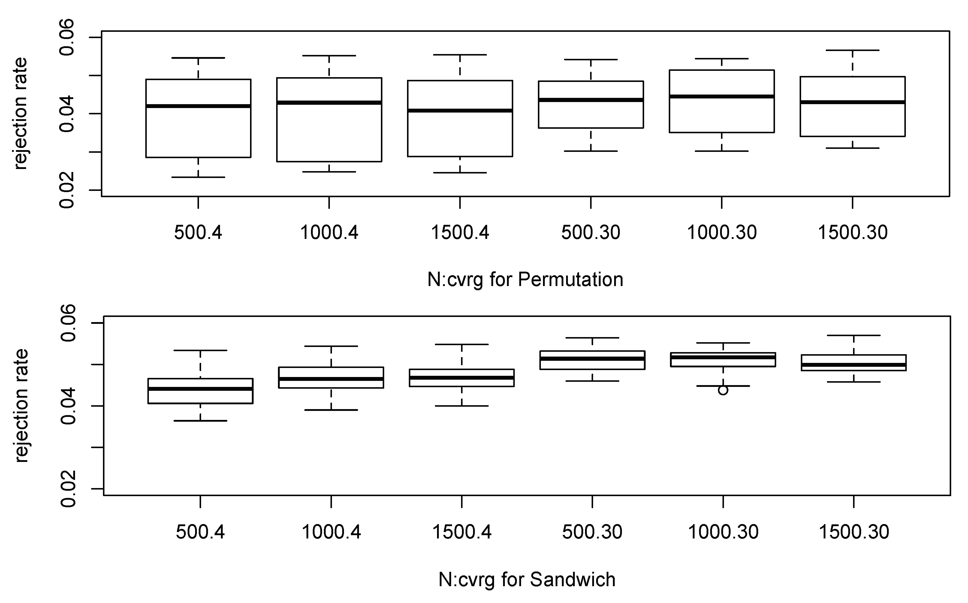
Figure 1 shows boxplots of the null simulations. The permutation method appears to have more variability of the empirical rejection rates over different configurations and to have the smaller empirical rejection rates compared to the proposed robust score test based on the sandwich variance estimator. When the sample size was small as 500 and the coverage was 4×, the permutation-based test had less than 2.5% rejection rate though the desired value is 5%. The smallest empirical rejection rate for the proposed robust test was greater than 3.5%, and it appears the empirical rejection rates become closer to 5% as the sample size increases. If the coverage is 30× or higher, then the estimated posterior probabilities in our approach are close to zero-or-one and most inferred genotypes are quite clear. When the coverage was 30×, our proposed test seems to well control the type I error rates regardless of other parameter settings as expected.

Table 1. Empirical rejection rates under null settings for level $1\times {10}^{-2},1\times {10}^{-3},1\times {10}^{-4}$, and $1\times {10}^{-5}$.

Method (cvrg)	$1\times {10}^{-2}$	$1\times {10}^{-3}$	$1\times {10}^{-4}$	$1\times {10}^{-5}$
Permutation (4×)	$7.13\times {10}^{-3}$	$6.14\times {10}^{-4}$	$4.44\times {10}^{-5}$	0
Permutation (30×)	$7.73\times {10}^{-3}$	$7.08\times {10}^{-4}$	$6.11\times {10}^{-5}$	$5.56\times {10}^{-6}$
Sandwich (4×)	$8.34\times {10}^{-3}$	$6.89\times {10}^{-4}$	$4.44\times {10}^{-5}$	$5.56\times {10}^{-6}$
Sandwich (30×)	$1.02\times {10}^{-2}$	$1.01\times {10}^{-3}$	$8.75\times {10}^{-5}$	$8.33\times {10}^{-6}$

shows the empirical rejection rates under the null settings by combining our simulation results for the lower level of significance.

3.1.2. Simulation Study for Statistical Power

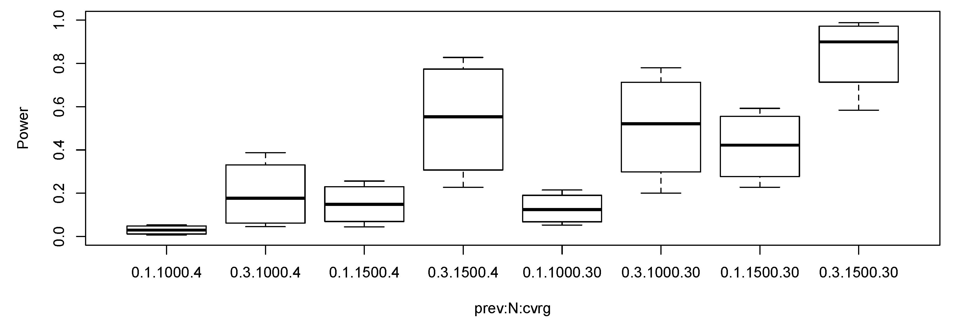
We used the same parameter settings as in the null simulation study. Additionally, we set multiplicative genetic relative risks vector $(1,1.5,{1.5}^2)$ in the alternative parameter configurations. In the alternative simulations, we calculated empirical rejection rates under Bonferroni corrected level of significance, that is, $5\times {10}^{-8}$. Figure 2 shows the boxplots of empirical power under various alternative settings. We removed the results when the sample size was 500 or the minor allele frequency was 0.05 since all the rejection rates were small in Figure 2. It appears interesting that the power of the proposed test when the coverage was 4× and the sample size was 1500 is higher than the power of the test when the coverage was 30× and the sample size was 1000. If the two design costs are similar, then the low-coverage with more samples seems more effective than the high-coverage with less samples.

Table 2. Empirical rejection rates under alternative hypothesis. The level of significance was set as $5\times {10}^{-8}$.

Coverage	Total Sample Size	Covariate	${\mathit{\beta }}_{\mathit{w}}$	Naive	Proposed
4	1000	Normal mixture	0	0.102	0.113
4	1000	Normal mixture	1	0.233	0.261
4	1000	Single normal	0	0.190	0.277
4	1000	Single normal	1	0.269	0.374
4	1500	Normal mixture	0	0.398	0.429
4	1500	Normal mixture	1	0.657	0.701
4	1500	Single normal	0	0.626	0.741
4	1500	Single normal	1	0.736	0.840
30	1000	Normal mixture	0	0.384	0.355
30	1000	Normal mixture	1	0.617	0.603
30	1000	Single normal	0	0.622	0.637
30	1000	Single normal	1	0.734	0.760
30	1500	Normal mixture	0	0.792	0.761
30	1500	Normal mixture	1	0.959	0.954
30	1500	Single normal	0	0.933	0.939
30	1500	Single normal	1	0.978	0.978

summarizes statistical power of our proposed method and a naive approach. The naive approach uses uncertain genotypes by the maximum posterior probability classification rule [29]. The standard logistic regression was applied to the uncertain genotypes. As expected, the proposed robust method shows higher power than the naive approach when the sequencing coverage is as low as 4×. When the sequencing coverage is high as 30×, two approaches show similar performance in terms of statistical power.

3.2. Real Data Analysis

The proposed robust generalized score test was applied to the pharmacogenomics data consisting of 400 epilepsy patients [22]. The data were collected from several epilepsy clinics in Korea and were genotyped for whole-exomes by NGS experiments [30]. All study participants followed the criteria in [31] if the participants had drug-resistant (case group) or drug-responsive (control group) epilepsy. We defined the drug resistance as the occurrence of at least four unprovoked seizures during the past one year at the time of recruitment, with trials of two or more appropriate antiepileptic drugs (AEDs) at maximal tolerated doses. Patients who underwent surgical treatment for drug-resistant epilepsy were classified as having drug-resistant epilepsy, regardless of the surgical outcome. We excluded some patients from the study if they were frequently in poor compliance with AED therapy and had reported seizures with a questionable semiology. In addition, we defined the drug responsiveness as complete freedom from seizures for at least one year up to the date of the last follow-up visit.

We included two non-genetic covariates in our association analysis. The two covariates were age of patient and duration of epileptic seizures. The age variable was definitely independent of genetic information, whereas duration variable may be associated with genetic variables. Due to the relatively small sample size 400, we did not expect to find a significantly associated SNP controlling for the two covariates. Therefore, instead of reporting a genome-wide association study, we illustrated the results of a SNP with low read depths and a SNP with high read depths. For the low read depths example, we selected a SNP from chromosome 1, which is $rs3811406$. The distribution of read depths for the SNP was summarized in

Table 3. Distribution of read depths at $rs3811406$.

Read Depth v	$\mathit{v}\le 5$	$5<\mathit{v}\le 10$	$10<\mathit{v}\le 30$	$\mathit{v}>30$	Total
Frequency	43	86	95	176	400
Proportion	0.1075	0.215	0.2375	0.44	1

. More than 10% of the sample had five or less read depths and more than 30% of the sample had 10 or less read depths at the SNP. When applying our proposed mixture-based association test, the test statistic value was $z_R=2.864$ and the p-value was $p=4.183\times {10}^{-3}$, while the standard logistic regression analysis using pooled genotype calls had $z=2.601$ and the p-value $p=9.30\times {10}^{-3}$ that was more than twice the p-value of the proposed robust test.

In addition, we applied our proposed test to SNP $rs4915154$ at which all patients had 13× or higher read depths and 85% patients had 25× or higher read depths. For this SNP, the proposed robust test statistic was $z_R=2.940$ with p-value $=3.28\times {10}^{-3}$ and the multiple logistic regression with the pooled genotype calls reported $z=2.963$ with p-value $=3.05\times {10}^{-3}$. The two results were quite close, as expected, due to high read depths at the SNP.

4. Discussion and Conclusions

In the present study, we developed the mixture-based genetic association tests adjusting the effects of non-genetic covariates in low-coverage NGS data. In order to construct a robust test statistic under model misspecification, we derived the sandwich variance estimator of the mixture model. The proposed test statistic is calculated from allele read counts and read depths instead of inferred genotypes so that we can apply this association test to low-coverage NGS data controlling for non-genetic covariates without external imputation or elimination of uncertain genotypes. Another important issue that we addressed in the present study is that the proposed test takes account of potential dependence between latent genotypes and the non-genetic covariates. Regarding computational cost, our proposed method is efficient because it is a generalized score test that uses the estimates of the parameters only under the null hypothesis of no association. When the sequencing depth is 4×, it takes around 1.2 s for sample size 500, 4 s for sample size 1000, and 9 s for sample size 1500 to simulate a dataset and to calculate both test statistics $Z_{AP}$ and $Z_R$. When the sequencing depth is 30×, it takes approximately 0.13 s for sample size 500, 0.3 s for sample size 1000, and 0.53 s for sample size 1500. Time for these computations is measured based on a single core work of a 3.5 GHz Intel Xeon processor. As illustrated in the real data analysis section, the read depth is not a fixed constant. Therefore, the computational time for real data is usually less than that for the coverage 4× simulation setting. We used statistical software R, which is known to be slow. It would be computationally beneficial to run our proposed methods in other faster program languages for a high-dimensional genome-wide association study.

We applied the penalized likelihood method to avoid singularity of information matrix when calculating the proposed score test statistic. Therefore, the penalty term is not necessary for a non-zero estimate of the error parameter. During our work, we fixed the degree of penalization $C=1$, $a_{ϵ}=0.01$, and $b_{ϵ}=0.99$ that implies 1% of allele read error as prior information. This parameter choice does not affect the proposed test statistic much since the likelihood function is merely changed when the sample size is greater than 500. It may be of interest to find optimal values for the parameters of the penalty term.

The simulation study confirms that the type I error rates of the proposed test are well controlled under the various parameter settings. The proposed robust test appears to perform better than the permutation based approach. Simulation results indicate that coverage 4× with sample size 1500 shows higher power as compared to coverage 30× with sample size 1000. Our method can be applied to an NGS experimental design by simulations to select coverage and sample size given a fixed amount of budget.

We presented a real data example in which the proposed test and multiple logistic regression results are similar to one another if the sequencing depth is high, whereas the test results may differ when the sequencing depth is low. This might have been caused because the proposed test is an extension of the multiple logistic regression with the unobserved latent genotype predictor. If the sequencing depth is high enough to call accurate genotypes, then our probability model becomes identical to the probability model of the multiple logistic regression. It would be more beneficial to compare with the previous methods by evaluating our proposed methods using a larger sized public dataset.

In this work, we focused on a single variant association test while controlling covariates. By adopting a multivariate mixture model, the proposed method can be extended to the multi-variant genetic association test including covariates. We can also extend the present method to differential genotype misclassifications.

References

- Wu, M.C.; Lee, S.; Cai, T.; Li, Y.; Boehnke, M.; Lin, X. Rare-variant association testing for sequencing data with the sequence kernel association test. Am. J. Hum. Genet. 2011, 89, 82–93. [Google Scholar] [CrossRef] [Green Version]
- Cirulli, E.T.; White, S.; Read, R.W.; Elhanan, G.; Metcalf, W.J.; Tanudjaja, F.; Fath, D.M.; Sandoval, E.; Isaksson, M.; Schlauch, K.A.; et al. Genome-wide rare variant analysis for thousands of phenotypes in over 70,000 exomes from two cohorts. Nat. Commun. 2020, 11, 542. [Google Scholar] [CrossRef]
- Lakiotaki, K.; Kanterakis, A.; Kartsaki, E.; Katsila, T.; Patrinos, G.P.; Potamias, G. Exploring public genomics data for population pharmacogenomics. PLoS ONE 2017, 12, e0182138. [Google Scholar] [CrossRef] [PubMed]
- Patrinos, G.P.; Giannopoulou, E.; Katsila, T.; Tsermpini, E.E.; Mitropoulou, C. Integrating next-generation sequencing in the clinical pharmacogenomics workflow. Front. Pharmacol. 2019, 10, 384. [Google Scholar]
- Celesti, F.; Celesti, A.; Wan, J.; Villari, M. Why Deep Learning Is Changing the Way to Approach NGS Data Processing: A Review. IEEE Rev. Biomed. Eng. 2018, 11, 68–76. [Google Scholar] [CrossRef]
- Le, N.Q.K.; Yapp, E.K.Y.; Nagasundaram, N.; Chua, M.C.H.; Yeh, H.Y. Computational identification of vesicular transport proteins from sequences using deep gated recurrent units architecture. Comput. Struct. Biotechnol. J. 2019, 17, 1245–1254. [Google Scholar] [CrossRef]
- Tripathi, R.; Sharma, P.; Chakraborty, P.; Varadwaj, P.K. Next-generation sequencing revolution through big data analytics. Front. Life Sci. 2016, 9, 119–149. [Google Scholar] [CrossRef]
- Cirillo, D.; Valencia, A. Big data analytics for personalized medicine. Curr. Opin. Biotechnol. 2019, 58, 161–167. [Google Scholar] [CrossRef]
- Sims, D.; Sudbery, I.; Ilott, N.E.; Heger, A.; Ponting, C.P. Sequencing depth and coverage: Key considerations in genomic analyses. Nat. Rev. Genet. 2014, 15, 121–132. [Google Scholar] [CrossRef]
- Song, K.; Li, L.; Zhang, G. Coverage recommendation for genotyping analysis of highly heterologous species using next-generation sequencing technology. Sci. Rep. 2016, 6, 35736. [Google Scholar] [CrossRef] [Green Version]
- Gordon, D.; Finch, S.J.; Nothnagel, M.; Ott, J. Power and sample size calculations for case-control genetic association tests when errors are present: Application to single nucleotide polymorphisms. Hum. Hered. 2002, 54, 22–33. [Google Scholar] [CrossRef]
- Ahn, K.; Haynes, C.; Kim, W.; Fleur, R.S.; Gordon, D.; Finch, S.J. The effects of SNP genotyping errors on the power of the Cochran-Armitage linear trend test for case/control association studies. Ann. Hum. Genet. 2007, 71, 249–261. [Google Scholar] [CrossRef]
- Kim, W.; Londono, D.; Zhou, L.; Xing, J.; Nato, A.Q.; Musolf, A.; Matise, T.C.; Finch, S.J.; Gordon, D. Single-variant and multi-variant trend tests for genetic association with next-generation sequencing that are robust to sequencing error. Hum. Hered. 2012, 74, 172–183. [Google Scholar] [CrossRef] [Green Version]
- Hou, L.; Sun, N.; Mane, S.; Sayward, F.; Rajeevan, N.; Cheung, K.; Cho, K.; Pyarajan, S.; Aslan, M.; Miller, P. Impact of genotyping errors on statistical power of association tests in genomic analyses: A case study. Genet. Epidemiol. 2017, 41, 152–162. [Google Scholar] [CrossRef] [Green Version]
- Consortium, G.P. An integrated map of genetic variation from 1092 human genomes. Nature 2012, 491, 56. [Google Scholar]
- Le, S.Q.; Durbin, R. SNP detection and genotyping from low-coverage sequencing data on multiple diploid samples. Genome Res. 2011, 21, 952–960. [Google Scholar] [CrossRef] [Green Version]
- Li, Y.; Sidore, C.; Kang, H.M.; Boehnke, M.; Abecasis, G.R. Low-coverage sequencing: Implications for design of complex trait association studies. Genome Res. 2011, 21, 940–951. [Google Scholar] [CrossRef] [Green Version]
- Kim, W.; Gordon, D.; Sebat, J.; Kenny, Q.Y.; Finch, S.J. Computing power and sample size for case-control association studies with copy number polymorphism: Application of mixture-based likelihood ratio test. PLoS ONE 2008, 3, e3475. [Google Scholar] [CrossRef]
- Barnes, C.; Plagnol, V.; Fitzgerald, T.; Redon, R.; Marchini, J.; Clayton, D.; Hurles, M.E. A robust statistical method for case-control association testing with copy number variation. Nat. Genet. 2008, 40, 1245. [Google Scholar] [CrossRef] [Green Version]
- Kim, S.Y.; Li, Y.; Guo, Y.; Li, R.; Holmkvist, J.; Hansen, T.; Pedersen, O.; Wang, J.; Nielsen, R. Design of association studies with pooled or un-pooled next-generation sequencing data. Genet. Epidemiol. 2010, 34, 479–491. [Google Scholar] [CrossRef] [Green Version]
- Gordon, D.; Finch, S.J.; De La Vega, F. A new expectation-maximization statistical test for case-control association studies considering rare variants obtained by high-throughput sequencing. Hum. Hered. 2011, 71, 113–125. [Google Scholar] [CrossRef]
- Kim, W.; Kim, Y.H. Genetic association tests when a nuisance parameter is not identifiable under no association. Commun. Stat. Appl. Methods 2017, 24, 663–671. [Google Scholar] [CrossRef]
- Kim, W. Transmission Disequilibrium Tests Based on Read Counts for Low-Coverage Next,-Generation Sequence Data. Hum. Hered. 2015, 80, 36–49. [Google Scholar] [CrossRef]
- Chen, H.; Chen, J.; Kalbfleisch, J.D. A modified likelihood ratio test for homogeneity in finite mixture models. J. R. Stat. Soc. Ser. B 2001, 63, 19–29. [Google Scholar] [CrossRef]
- Zhou, H.; Pan, W. Binomial mixture model-based association tests under genetic heterogeneity. Ann. Hum. Genet. 2009, 73, 614–630. [Google Scholar] [CrossRef] [Green Version]
- Dempster, A.P.; Laird, N.M.; Rubin, D.B. Maximum likelihood from incomplete data via the EM algorithm. J. R. Stat. Soc. Ser. B 1977, 39, 1–22. [Google Scholar]
- White, H. Maximum Likelihood Estimation of Misspecified Models. Econometrica 1982, 50, 1–25. [Google Scholar] [CrossRef]
- Sidak, Z.; Sen, P.K.; Hajek, J. Theory of Rank Tests; Academic Press: San Diego, CA, USA, 1999. [Google Scholar]
- Anderson, T.W. An Introduction to Multivariate Statistical Analysis; Wiley: New York, NY, USA, 1962. [Google Scholar]
- Kang, K.W.; Kim, W.; Cho, Y.W.; Lee, S.K.; Jung, K.Y.; Shin, W.; Kim, D.W.; Kim, W.J.; Lee, H.W.; Kim, W. Genetic characteristics of non-familial epilepsy. PeerJ 2019, 7, e8278. [Google Scholar] [CrossRef]
- Kim, M.-K.K.; Moore, J.H.; Kim, J.K.; Cho, K.H.; Cho, Y.W.; Kim, Y.S.; Lee, M.C.; Kim, Y.O.; Shin, M.H. Evidence for epistatic interactions in antiepileptic drug resistance. J. Hum. Genet. 2011, 56, 71–76. [Google Scholar] [CrossRef] [Green Version]
Figure 1.
Boxplot of the empirical rejection rates under the null hypothesis.
Figure 2.
Boxplots of statistical power of the proposed robust test under the alternative settings. The level of significance was set as . The notation 0.1.1000.4 represents prevalence 0.1, total sample size 1000, and coverage 4×.