WINkNN: Windowed Intervals’ Number kNN Classifier for Efficient Time-Series Applications
by
 ,
,
Chris Lytridis
1 ,
,
Anna Lekova
2, 
Christos Bazinas
1, 
Michail Manios
1 and
Vassilis G. Kaburlasos
1,*
1
HUMAIN-Lab, International Hellenic University (IHU), 65404 Kavala, Greece
2
Institute of Robotics, Bulgarian Academy of Sciences, 1113 Sofia, Bulgaria
*
Author to whom correspondence should be addressed.
Mathematics 2020, 8(3), 413; https://0-doi-org.brum.beds.ac.uk/10.3390/math8030413
Submission received: 23 February 2020
/
Revised: 9 March 2020
/
Accepted: 9 March 2020
/
Published: 13 March 2020
(This article belongs to the Special Issue Lattice Computing: A Mathematical Modelling Paradigm for Cyber–Physical System Applications)
Abstract
:Our interest is in time series classification regarding cyber–physical systems (CPSs) with emphasis in human-robot interaction. We propose an extension of the k nearest neighbor (kNN) classifier to time-series classification using intervals’ numbers (INs). More specifically, we partition a time-series into windows of equal length and from each window data we induce a distribution which is represented by an IN. This preserves the time dimension in the representation. All-order data statistics, represented by an IN, are employed implicitly as features; moreover, parametric non-linearities are introduced in order to tune the geometrical relationship (i.e., the distance) between signals and consequently tune classification performance. In conclusion, we introduce the windowed IN kNN (WINkNN) classifier whose application is demonstrated comparatively in two benchmark datasets regarding, first, electroencephalography (EEG) signals and, second, audio signals. The results by WINkNN are superior in both problems; in addition, no ad-hoc data preprocessing is required. Potential future work is discussed.
1. Introduction
A cyber–physical system (CPS) has been defined as a device with sensing as well as reasoning capacities [1,2]. Strategic initiatives regarding CPSs include “Industrie 4.0” in Germany, the “Industrial Internet of Things (IIoT)” in the United States, and “Society 5.0” in Japan [3]. CPSs typically focus on multidisciplinary applications in healthcare, agriculture, and food supply, manufacturing, energy and critical infrastructures, transportation, logistics, security, and, lately, education [4]. Our interest here is in CPSs regarding human-robot interaction.
There is a need for supporting CPSs with mathematical models that involve both sensory data and structured software data toward improving CPS performance during their interaction with humans. However, a widely acceptable mathematical modelling framework is currently missing. In response, the lattice computing (LC) paradigm has been introduced [1,5] for hybrid mathematical modelling based on mathematical lattice theory that unifies rigorously numerical data and non-numerical data; the latter may include (lattice ordered) logic values, sets, symbols, and trees/graphs. More specifically, the cyber and physical components of a CPS are modelled involving non-numerical and numerical data, respectively, in any combination. An additional advantage of lattice computing is its capacity to calculate with semantics represented by a lattice (partial) order relation.
Human-robot interaction is, typically, driven by behavioral patterns including auditory and/or visual signals. Visual stimuli are very common in human-robot interaction applications, and are often treated as time-series data. For example, in [6] recognition of time-series segments is used to treat hand gestures as natural language processing; furthermore, in [7] time series data are used for nod detection. Recent work has considered electroencephalography (EEG) signals toward improving decision-making, and the results have been encouraging [8,9,10]. Another important modality in human-robot interaction is speech [11]. More specifically, humans use a number of linguistic social cues (i.e., words or phrases that reveal sympathy, empathy, encouragement etc.,) which could be especially useful toward an effective human-robot interaction.
Automated emotion recognition is important in human-robot interaction, for instance regarding the design of smart collaborative or assistive robots. Current aspects and future directions in emotion recognition using machine learning is shown in [12,13], where different machine learning techniques are proposed for recognizing emotions from physiological signals (EEG in particular). Note that data preprocessing and feature selections both are critical as well as computationally expensive. Table 3 in [12] presents some of the most popular features extracted from time-series including temporal, statistical, spectral, linear, and/or non-linear features. Classifiers used to recognize emotional states, typically, regard supervised learning including k nearest neighbor (kNN) [14,15,16,17], support vector machine (SVM) [17,18,19], Naive–Bayes (NB) [17], quadratic discriminant analysis (QDA) [20], artificial neural networks [21,22]. Furthermore, unsupervised and semi-supervised learning algorithms are also used [12].
Summarizing the bibliography research, both ad hoc feature extraction and classification of big data impose large feature dimensions resulting in high computational costs for training. To counter the aforementioned problems we propose using intervals’ numbers (INs) in the framework of lattice computing (LC). Recall that LC has been defined as “an evolving collection of tools and methodologies that process lattice ordered data including logic values, numbers, sets, symbols, graphs, etc.,” [23,24]. We point out that LC is not merely an algorithm but rather it is an information processing paradigm. LC models are expected to be useful in CPS applications including human-robot interaction because they can (1) deal with both numerical data (regarding physical system components) as well as with non-numerical data (regarding cyber system components), (2) compute with semantics, represented by a partial-order relation, (3) rigorously deal with ambiguity represented by information granules, (4) naturally engage logic and reasoning, and (5) process data fast. LC suggests useful instruments for analysis and design of new technologies including formal concepts [25,26], type-2 fuzzy sets [23,27], and other. In the context of the LC framework, intervals’ numbers, or INs for short, have been studied as explained next.
An IN is a mathematical object that can represent either a fuzzy interval or a distribution of samples [2,28,29,30]. Applications of INs have been reported to neural networks (NNs) as well as to fuzzy inference systems (FIS) [23,31,32,33,34,35]. INs are engaged here for massive data representation in time-series as explained in the following.
An advantage of an IN is its capacity to represent data statistics of all-orders using few numbers; more specifically, L numbers are used to define L intervals; hence, a significant data reduction may result in a capacity to process big data fast. Furthermore, no feature extraction is necessary since the all-order statistics, represented by an IN, are implicitly employed as features. An IN-based k nearest neighbor (kNN) scheme was introduced for classification by fuzzy lattice reasoning (FLR) in [5]. However, a drawback of the latter work, regarding classification of time-series using INs, has been the suppression of the “time dimension” because of the representation of a whole time-series by a single IN. A novelty of this work is a recovery of the “time dimension” by the windowed IN-based k nearest neighbor classifier, or WINkNN for short, which is applied comparatively on two different datasets, namely (a) a human brain EEG dataset for emotion recognition, and (b) an audio dataset for word classification.
The remainder of the paper is structured as follows. Section 2 summarizes the useful mathematical instruments. Section 3 presents the methods as well as the datasets used in our experiments. Section 4 presents experiments and results as well as a discussion. Finally, Section 5 concludes by summarizing the contribution of this work; potential future work is also delineated.
2. Mathematical Background
Given a lattice (L,⊑), a valuation is defined as a real function v: L→R that satisfies v(x⊓y) + v(x⊔y) = v(x) + v(y), x,y∈L. A valuation is called monotone if x ≤ y ⇒ v(x) ≤ v(y), and positive if x < y ⇒ v(x) < v(y). A positive valuation function v: L→R in (L,⊑) defines a metric distance function given by d(x,y) = v(x⊔y) − v(x⊓y). Extensions to Cartesian products follow.
A lattice (L,⊑) may be the Cartesian product of N constituent lattices (Li,⊑), i = 1,…,N, i.e., (L,⊑) = (L1,⊑) × … × (LN,⊑), where (x1,…,xN) = x ⊑ y = (y1,…,yN) ⇔ x1⊑y1,…,xN⊑yN. Positive valuation functions vi: Li→R in the constituent lattices (Li,⊑), i = 1,…,N, respectively, define a parametric Minkowski metric function in the product lattice (L,⊑) = (L1,⊑) × … × (LN,⊑) given by
where xi, yi∈Li, i = 1,…,N, x = (x1,…,xN), y = (y1,…yN). Next, we consider metrics in a lattice hierarchy.
A hierarchy of lattices in three levels is presented next, resulting in the lattice of Intervals’ Numbers [34,36,37]. For each level, metric distance functions are introduced.
Level-0; The Lattice (R, ≤) of Real Numbers: Assume the lattice (R,≤) of real numbers. The greatest lower bound of two numbers x and y is the smallest of the two, denoted by x˄y, whereas the least upper bound of two numbers is the greatest of the two, denoted by x˅y. Positive valuation function v: R→R in lattice (R,≤) is any strictly increasing function. For instance, choosing v(x) = x it follows that the distance between two real numbers x and y equals d(x,y) = v(x˅y) − v(x˄y) = x˅y − x˄y = |x−y|. Extending to the N-dimensional Euclidean space (RN,⊑), with v(x) = x in every dimension, from Equation (1) there follows the Minkowski metric d(x,y;p) = known in the literature as Lp metric. In particular, the L1 metric d(x,y;1) = is known as Hamming distance; the L2 metric d(x,y;2) = is known as Euclidean distance; furthermore; the L∞ metric equals d(x,y;∞) = max{|x1 − y1|,…,|xN − yN|}.
Level-1; The Lattice (Ι1, ≤) of Intervals: In the lattice (R,≤) of real numbers, any strictly decreasing function is a dual isomorphic function. Consider the partially ordered lattice (Ι1, ⊑) of intervals in the lattice (R,≤). The greatest lower bound of two intervals [a, b] and [c, e] is given by [a, b]⊓[c, e] = [a˅c, b˄e] if a˅c ≤ b˄e, and [a, b]⊓[c, e] = ∅ = [+∞, −∞] if a˅c > b˄e; whereas, the corresponding least upper bound is given by [a, b]⊔[c, e] = [a˄c, b˅e].
Given (a) a positive valuation function v: R→R, and (b) a dual isomorphic function θ: R→R in (R,≤), a positive valuation v1: R×R→R in the corresponding lattice (R×R,≥×≤) of generalized intervals is defined by v1([a, b]) = v(θ(a)) + v(b). Therefore, a metric distance in (R×R,≥×≤) is given by:
d1([a, b],[c, e]) = v1([a, b]⊔[c, e]) − v1([a, b]⊓[c, e]) = v(θ(a)˅θ(c)) − v(θ(a)˄θ(c)) + v(b˅e) − v(b˄e)
In conclusion, the metric d1(.,.), given by Equation (2), is valid in sublattice (Ι1,⊑), which is embedded to the superlattice (R×R,≥×≤).
Level-2; The Lattice (F1, ≤) of Intervals’ Number (INs): A Generalized Intervals’ Number, or GIN for short, is defined as a function f: [0, 1]→(R×R,≥×≤) where (R×R,≥×≤) is a lattice of Generalized Intervals. Let G be the set of GINs; then, the (G,⊑) is a lattice, as a (non-numerable) Cartesian product of complete lattices (R×R,≥×≤). Next, the interest focuses on the sublattice of INs.
An intervals’ number, or IN for short, is defined as a function F: [0, 1]→I1 that satisfies:
The set F1 of INs is a partially ordered lattice denoted as (F1,≼). An IN is interpreted as a grain of information [36]. In particular, it has been shown that (F1,≼) is a metric lattice [38] whose metric function is given by
where the integrable function is defined by Equation (2). For L = there follows a Minkowski metric given by Equation (1).
Parametric functions v(.) and θ(.) may introduce tunable non-linearities whose parameters can be estimated optimally. In this work, toward reducing complexity during optimization, we consider functions v(.) and θ(.) with only two parameters per function; in particular, we consider exclusively linear parametric functions v(.) and θ(.):
v(x) = v1x + v0,
θ(x) = θ1x + θ0,
3. Methods and Datasets
This section deals with data representation issues as well as the windowed IN kNN, or WINkNN for short, classifier. It also presents the datasets to be employed in the next section.
3.1. Intervals’ Numbers (INs) and Time-Series Representation Based on INs
Probability and possibility distributions have been studied comparatively in the literature [39,40]. Furthermore, a possibilistic interpretation has been proposed for an IN [38] followed by a probabilistic interpretation [37]. In conclusion, an IN was established as a mathematical object, which can be interpreted either probabilistically or possibilistically [30].
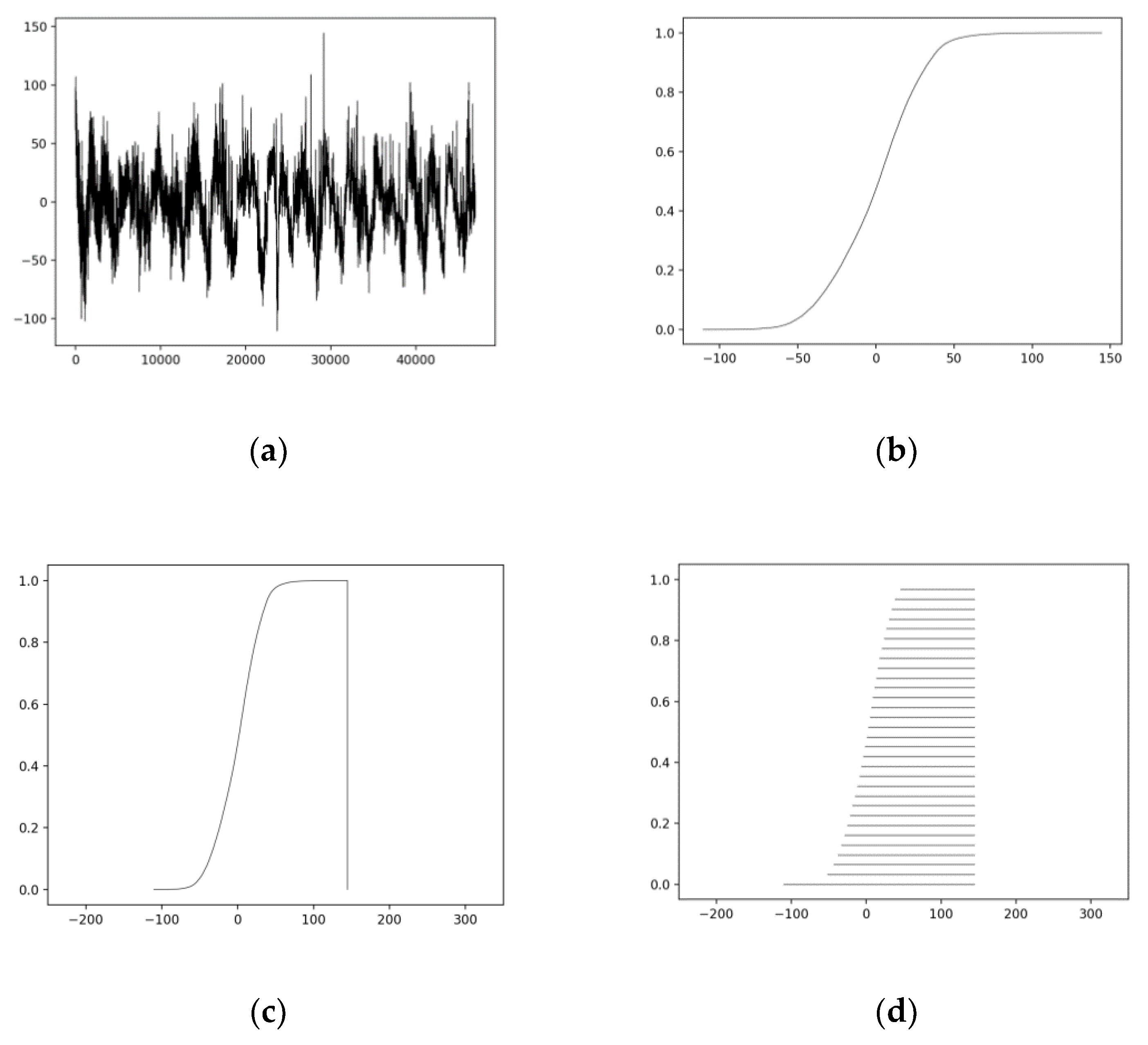
Recall that an IN can be represented either as a function F(x) = , namely membership-function-representation or, equivalently, as set of intervals Fh, h[0, 1], namely interval-representation. We point out the potential of an IN to represent time-series big data. More specifically, the big data here regards the (time-series) samples. For instance, consider the EEG time-series signal shown in Figure 1a. Figure 1b shows the corresponding distribution function, regarding the time-series samples values, induced by algorithm distrIN [2]. Figure 1c displays the membership-function-representation of IN F; note that the latter matches the distribution function in Figure 1b. Finally, Figure 1d shows the equivalent, interval-representation of IN F using L = 32 intervals, where the reason for using L = 32 is explained in [30]. In conclusion, using only L = 32 numbers that define L = 32 intervals, we can potentially represent a distribution of samples. In the aforementioned sense, an IN with fairly few (i.e., L = 32) numbers can represent the distribution of orders of magnitude more numbers.
In all previous works, a whole time-series signal has been represented by a single IN, e.g., [2,5]. However, the latter representation suppresses the “time dimension” which constitutes a significant information content. To recover the “time dimension,” two alternatives have been examined here, namely Alternative 1 (AL1) and Alternative 2 (AL2), respectively, as explained in the following.
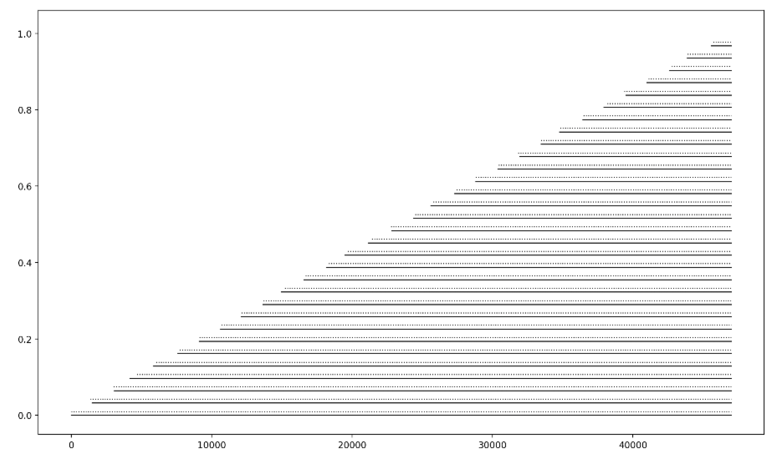
First, Alternative AL1 computes the cumulative sum (over time) of the samples’ magnitude, normalized to [0, 1]. Figure 2 displays two INs induced from two EEG signals in two different classes, respectively, by Alternative AL1. Although time has been taken into account, there is no significant difference between the two INs in Figure 2 because the large number of involved samples resulted in very similar IN shapes. Hence, the distance between the two INs (computed by Equation (3)) is negligible. The latter explains the poor classification results recorded in experiments we have carried out using AL1. Therefore, Alternative AL1 was abandoned.
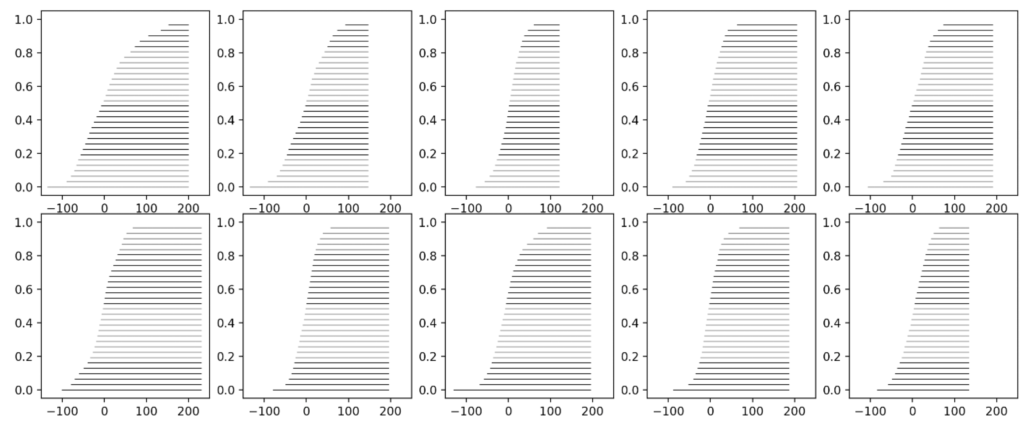
Second, Alternative AL2 recovers (partly) the time dimension by partitioning the original time-series signal into consecutive windows; then, computing one IN per window. More specifically, the time-series signal is partitioned in a number N of windows of equal length; then, from all the data in a window, one IN is induced per window by algorithm distrIN [2]. For instance, from the EEG signal in Figure 1a, using N = 10 windows, the ten INs of Figure 3 were induced. Such a (partial) recovery of time has improved classification performance as demonstrated below.
3.2. The Datasets
Two different datasets have been engaged regarding, first, electroencephalography (EEG) data and, second, audio data, as explained in the following.
3.2.1. Electroencephalography (EEG) Dataset
We considered the SEED dataset [41,42], which contains EEG data signals collected from 15 subjects (7 males and 8 females aged between 22 and 24 years old) while watching movie clips designed to elicit three types of emotions, namely “positive”, “neutral,” and “negative.” More specifically, each subject watched five clips for each types of emotion. The experiment was repeated three times. Therefore, the dataset included 3*5*15 = 225 trials per emotion. Note that the recording device was an EEG cap conforming to the international 10–20 system (for 62 channels); hence, for each trial (i.e., for each movie clip) there were 62 signals corresponding to the 62 channels, respectively. An EEG signal was sampled at 200 Hz resulting in time-series with 37,001 to 47,001 samples per time-series. Our objective was to recognize the emotional state, namely “positive,” “neutral,” or “negative,” of individuals using EEG signals.
Of the 62 channels recorded by the EEG cap’s electrodes, not all were used in our emotion recognition computational experiments. Efficient emotion recognition calls for prior channel selection in order to reduce computational complexity. More specifically, channel selection depends on the brain region involved in processing, given the stimulus. Previous studies have identified appropriate channel groups [42,43]. For comparison purposes, the five groups of channels proposed in [44], including four channels per group, were used in this work. More specifically, Table 1 shows the channel groups used in our classification experiments. In addition to the aforementioned five channel groups, the set-union of the channels in the five groups was also considered resulting in nine channels, namely FP1, FT8, T7,T8, TP7, PO7, FC2, FPZ, F8. We point out that each signal was decomposed into delta (δ), theta (θ), alpha (α), beta (β), and gamma (γ) frequency bands [45].
3.2.2. Audio Dataset
The objective here is spoken word classification using the Spoken Digits dataset [46], which contains 2000 recordings of English utterances of the ten digits “zero” to “nine” by four native English speakers. This dataset includes 200 signals per digit. Moreover, note that an audio signal was sampled at 8 KHz resulting in time-series with 1148 to 18,262 samples per time-series. Minimal silence was ensured by trimming the audio signal both at the beginning and at the end.
3.3. The Windowed Intervals’ Number kNN (WINkNN) Classifier
We assume a dataset including ntrn and ntst subjects for training and testing, respectively. In particular, the data regarding a single subject includes nch time-series (i.e., channels). A time-series is optimally partitioned, as described below, in N parts, or equivalently windows, of equal length.
Algorithm 1 describes the windowed intervals’ number kNN (WINkNN) classifier for training. In particular, an optimal set of parameters is computed in Algorithm 1 using the GENETIC optimization detailed in the next section. Note that Algorithm 1 implements “leave-one-out” training per individual chromosome. Next, Algorithm 2 details testing by the WINkNN classifier.
| Algorithm 1 Windowed Intervals’ Number kNN (WINkNN) classifier for training | |
| 0. | Let k be the (integer) parameter of the kNN classifier; let ncl be the total number of classes; let ntrn be the number of subjects for training; let nch be the number of channels per subject; let N be the number of windows per channel; a time-series in a channel is represented by an element F∈; let NG be the number of generations of the GENETIC algorithm; |
| 1. | m = 1; |
| 2. | while m < NG do |
| 3. | for i = 1 to ntrn do %this loop is executed per chromosome r∈{1,…,nr}; |
| 4. | Initialize (i.e., set to zero) the vector ClassCounter(1,…,ncl) ← (0,…,0); |
| 5. | for l = 1 to nch do |
| 6. | Calculate the set: kWinners(i,l) = D(Fi,l,Fj,l) that holds the indices of the k nearest neighbors to Fi,l∈ for j ≠ i; |
| 7. | Using the class labels of the k winners in the set kWinners(i,l), update (i.e., increase the corresponding entries of) vector ClassCounter(1,…,ncl); |
| 8. | end for |
| 9. | The subject i is classified to the class: ClassCounter(1,…,ncl); |
| 10. | Update the success rate (fitness) Qr per chromosome r∈{1,…,nr}; |
| 11. | end for |
| 12. | GENETIC optimization of the “2*2*N*nch + 1” parameters v0, v1, θ0, θ1 per window per channel as well as parameter k of the WINkNN classifier; |
| 13. | m ← m + 1; |
| 14. | end while |
| Algorithm 2 Windowed Intervals’ Number kNN (WINkNN) classifier for testing | |
| 0. | Let k be the (integer) parameter of the kNN classifier; let ncl be the total number of classes; let nch be the number of channels per subject; let N be the number of windows per channel; a time-series in a channel is represented by an element F∈; consider a subject F0∈ l∈{1,…, nch} for classification; |
| 1. | Initialize (i.e., set to zero) the vector ClassCounter(1,…,ncl) ← (0,…,0); |
| 2. | forl = 1 to nch do |
| 3. | Calculate the set: kWinners(l) = D(F0,l,Fj,l) that holds the indices of the k nearest neighbors to F0∈ l∈{1,…, nch}; |
| 4. | Update (i.e., increase the corresponding entries of) vector ClassCounter(1,…,ncl) by considering the class labels of the k winners in the set kWinners(l); |
| 5. | end for |
| 6. | The subject F0 is classified to the class: ClassCounter(1,…,ncl). |
3.4. GENETIC Optimization
As mentioned above, the distance between two INs is calculated based on the two parametric functions ν(x) and θ(x) per window per channel. The parameter values of the aforementioned functions affect the metric distance, and as a result, the classification performance changes. To determine an optimal set of parameters that maximizes classification performance, a GENETIC algorithm was employed as detailed next.
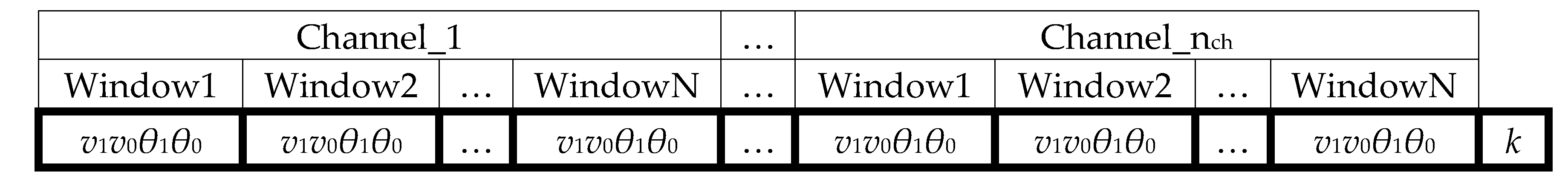
During an initialization step, a population of nr chromosomes was considered. Each chromosome represented the set of parameters for classification. More specifically, for linear ν(x) and θ(x) functions, there were two parameters per function (v1/v0 and θ1/θ0, respectively) that define slope and position. To enhance flexibility in tuning, we considered different pairs of functions ν(x) and θ(x) per window per channel. For example, to classify EEG signals with 9 channels, where each signal was partitioned in N = 5 windows, we used 2*2*5*9 = 180 parameters. Moreover, an additional parameter was used for the k value of the kNN classifier. Figure 4 shows the structure of a chromosome for nch channels and N windows per (time-series) signal.
An initial population of nr chromosomes (i.e., individuals) was randomly generated under constraints, namely the parametric functions ν(x) and θ(x) must be monotonically increasing and decreasing, respectively. Then, the fitness (i.e., cost) function of the GENETIC algorithm was computed as follows. Given ncl classes, the result of a classification cycle, regarding all the ntst subjects for testing, is a ncl × ncl confusion matrix B including classification percentages. In conclusion, the following fitness function was used per chromosome:
The cost function Qr indicates how well a set of parameters defines distances that improve classification. Initially, all individuals are evaluated and they are sorted according to cost. To speed up data processing, parallel processing was applied for the evaluation of the individuals. Next, the individual selection procedure was applied to replace the parental population using tournament selection followed by genetic crossover and mutation; in particular, crossover was applied with probability cxpb = 0.7, whereas mutation was applied with probability mutpb = 0.02.
4. Experiments and Results
Two different sets of experiments have been conducted to demonstrate the capacity of the proposed WINkNN classifier regarding, first, an emotion classification task using EEG signals and, second, a word classification task using auditory signals. In each experiment, a single subject was left out for testing; eventually, every subject was left out exactly once for testing. In the aforementioned manner we estimated the generalization capacity of the WINkNN classifier. For both datasets, during the GENETIC optimization, the parameter values nr = 200 and NG = 50 were selected empirically.
4.1. Electroencephalography (EEG) Signal Classification
An optimal number N of windows was estimated, in the first place. In particular, before any optimization, classification experiments were carried out for an increasing number of 2, 3, 4, 5, 10, 15, and 20 windows. Table 2 shows the corresponding classification results. It was observed that when signals were partitioned to more than 5 windows, there was no significant improvement in classification performance; moreover, the computational cost was increasing rapidly for more than 5 windows. In conclusion, we decided to use N = 5 windows.
Table 3 displays the results obtained by the WINkNN classifier comparatively with the results by alternative classification methods from the literature.
It can be seen that the classification performance of our proposed WINkNN classifier is comparable to more complex (therefore more computationally expensive) classification techniques that make use of the entire set of available cap electrodes and, in some cases, it is superior, especially when a small number of channels is used. Even though alternative approaches are based on feature extraction, our method operates on raw data—in other words, no ad hoc feature extraction has been carried out whatsoever. The windowed IN approach is also superior to the authors’ previous work where a single IN was used to represent the entire signal [5]. It was also observed during the experiments that WINkNN was robust in terms of the consistency of classification results. Despite the fact that EEG signals stemming even from the same subject in response to same stimuli are not repeatable, the aforementioned consistency of the WINkNN classifier was remarkable and attributed to the representation of a data distribution by an IN.
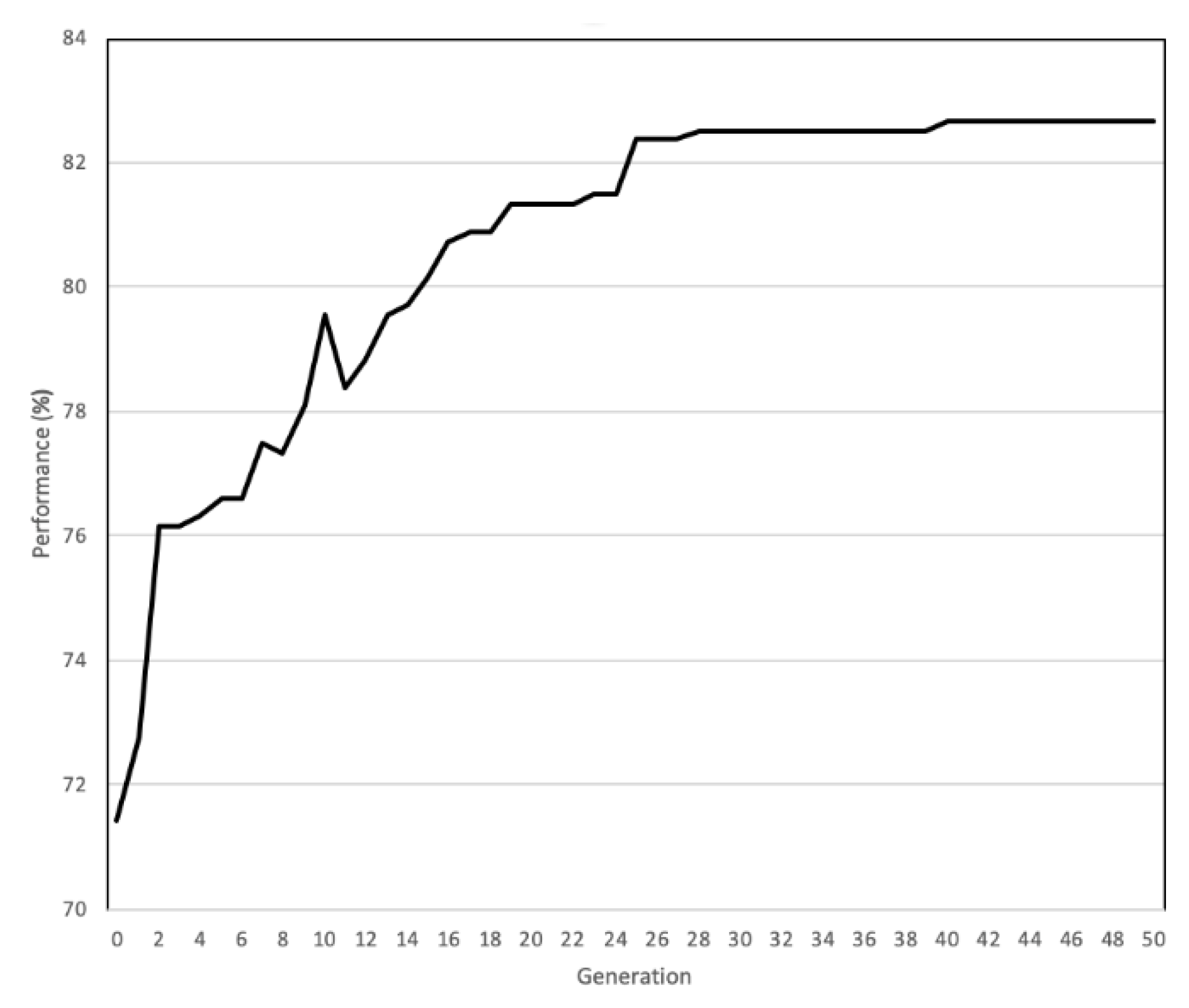
During GENETIC optimization, the parameter ranges v1∈[0,10], v0∈[−1500,1500], θ1∈[0,10], θ0∈[−1500,1500], k∈[4,10] were used; moreover, nch was either nch = 4 or nch = 9. Figure 5 shows an example of the improvement in classification performance resulting from the application of the GENETIC algorithm. Furthermore, Table 4 displays a set of optimal parameter values computed by GENETIC optimization for channel group G1, for all windows in all channels.
4.2. Audio Signal Classification
An optimal number N = 15 of windows was estimated by trial-and-error as in the previous section regarding EEGs; furthermore, one IN was induced per window. Three different experiments were carried out including: (a) 3 classes (spoken digits “0”, “5” and “9”), (b) 5 classes (spoken digits “0”, “3”, “5”, “7” and “9”), and (c) 10 classes for all ten spoken digits.
During GENETIC optimization, the parameter ranges v1∈[0,10], v0∈[−1000,1000], θ1∈[0,10], θ0∈[−1000,1000], k∈[4,10] were used; moreover, nch = 1. Table 5 shows the classification results by the WINkNN classifier compared to the authors’ previous results [50] (in brackets), where a time-series was represented by a single IN. For all aforementioned three class groups, the WINkNN classifier resulted in a superior improvement.
4.3. Discussion
The use of a single IN to represent a time-series ignores the “time dimension” of a time-series signal; more specifically, it considers solely the distribution of the signal samples. Nevertheless, with the proposed WINkNN classifier, the “time dimension” is (partly) recovered toward improving classification performance. The classification results here have confirmed a consistent improvement in classification performance because of the partition of a time-series to more than 1 window.
It is observed that the improvement is larger for the experiments with the audio signals than with the EEG signals. This was explained by the fact that the information content in audio signals is more dependent on time, as opposed to the EEG signals which are significantly affected by a number of concurrent brain activations. Note also that not only EEG signals are subject-specific, but also the data in the trials, even per subject, are not repeatable, resulting in a decrease of classification performance for the EEG signals in comparison to audio signals.
Partitioning the signals to N time windows multiplies the total number of parameters of the WINkNN classifier. The latter increases the search space for the GENETIC algorithm and makes convergence to an optimal set of parameters slower. However, significant benefits are retained with N time windows including: (a) Substantial data reduction, compared to the raw data, because of the employment of “N” INs per channel; hence, the proposed techniques emerge promising for big data applications. (b) Time consuming, ad hoc feature extraction is not necessary; instead, all-order statistics are used implicitly as features for tunable classification using the optimizable, parametric WINkNN classifier. (c) Fairly heavy computational overhead is required only once, during training.
We remark that recently published classification techniques from the literature have reported higher classification results than the WINkNN classifier on the SEED (EEG) dataset but at the expense of considerably more time for computation, using all 64 channels as well as all frequency bands; moreover, ad hoc features had to be defined [14].
5. Conclusions
The interest of this work was in time-series classification regarding human-robot interaction. Our proposed novelty was to represent “time” by an N-tuple of INs instead of by a single IN. A novel windowed IN-based kNN, namely WINkNN, classifier was introduced and applied to two different benchmark classification datasets, namely the SEED dataset and the Spoken Digit dataset regarding the recognition of emotional states based on EEG signals and the recognition of spoken digits based on audio signals, respectively. Extensive computational experiments have demonstrated, comparatively, a superior performance of the WINkNN classifier.
The proposed WINkNN classifier used raw (time-series) data; in other words, no ad hoc feature extraction was necessary. The latter is considered to be a major advantage toward transferring IN-based techniques to a wide range of applications. Moreover, the performance of the proposed method can be optimized, parametrically. The capability of the WINkNN classifier was attributed (a) to the capacity of an IN to represent statistics of all-orders; the latter are the “features” engaged implicitly, (b) to the capacity to optimize, parametrically, the distance function, and (c) to the consideration of time.
Because of its capacity for representing a distribution of samples, an IN can potentially represent big data. Hence, IN-based techniques emerge promising in big data applications. Potential future work may include various time-series applications to different domains such as medicine, physics, economics, agriculture, and elsewhere. The implicit employment of “all-order statistics” should also be studied. Further future work will pursue an engagement of INs with alternative architectures such as neural networks etc.
Author Contributions
Conceptualization, V.G.K. and A.L.; data curation, M.M.; formal analysis, V.G.K. and C.L.; funding acquisition, V.G.K.; investigation, M.M.; methodology, V.G.K., A.L., and C.L.; project administration, V.G.K.; resources, C.B.; software, C.L.; supervision, V.G.K., and A.L.; validation, C.L., C.B., and M.M.; visualization, M.M.; writing—original draft, C.L., C.B., and M.M.; writing—review and editing, V.G.K. and A.L. All authors have read and agree to the published version of the manuscript.
Funding
This project has received funding from the European Union’s Horizon 2020 research and innovation programme under the Marie Skłodowska-Curie grant agreement No 777720.
Conflicts of Interest
The authors declare no conflict of interest. The funders had no role in the design of the study; in the collection, analyses, or interpretation of data; in the writing of the manuscript, or in the decision to publish the results.
References
- Kaburlasos, V.G.; Vrochidou, E. Social Robots for Pedagogical Rehabilitation: Trends and Novel Modeling Principles. In Cyber-Physical Systems for Social Applications. Advances in Systems Analysis, Software Engineering, and High Performance Computing (ASASEHPC); Dimitrova, M., Wagatsuma, H., Eds.; IGI Global: Hershey, PA, USA, 2019; pp. 1–21. [Google Scholar]
- Kaburlasos, V.G.; Vrochidou, E.; Panagiotopoulos, F.; Aitsidis, C.; Jaki, A. Time Series Classification in Cyber-Physical System Applications by Intervals’ Numbers Techniques. In Proceedings of the 2019 IEEE International Conference on Fuzzy Systems (FUZZ-IEEE), New Orleans, LA, USA, 23–26 June 2019; pp. 1–6. [Google Scholar]
- Serpanos, D. The Cyber-Physical Systems Revolution. Computer 2018, 51, 70–73. [Google Scholar] [CrossRef]
- Cyber-Physical Systems for PEdagogical Rehabilitation in Special Education. Available online: https://cordis.europa.eu/project/rcn/212970_en.html (accessed on 7 October 2019).
- Vrochidou, E.; Lytridis, C.; Bazinas, C.; Papakostas, G.A.; Kaburlasos, V.G. Fuzzy Lattice Reasoning for Brain Signal Classification. J. Univ. Comput. Sci. 2019. under review. [Google Scholar]
- Simão, M.; Neto, P.; Gibaru, O. Using data dimensionality reduction for recognition of incomplete dynamic gestures. Pattern Recognit. Lett. 2017, 99, 32–38. [Google Scholar] [CrossRef]
- Wall, E.; Schillingmann, L.; Kummert, F. Online nod detection in human-robot interaction. In Proceedings of the 2017 26th IEEE International Symposium on Robot and Human Interactive Communication (RO-MAN), Lisbon, Portugal, 28 August–1 September 2017; pp. 811–817. [Google Scholar]
- Atkinson, J.; Campos, D. Improving BCI-based emotion recognition by combining EEG feature selection and kernel classifiers. Expert Syst. Appl. 2016, 47, 35–41. [Google Scholar] [CrossRef]
- Mohammadi, Z.; Frounchi, J.; Amiri, M. Wavelet-based emotion recognition system using EEG signal. Neural Comput. Appl. 2017, 28, 1985–1990. [Google Scholar] [CrossRef]
- Wang, X.-W.; Nie, D.; Lu, B.-L. Emotional state classification from EEG data using machine learning approach. Neurocomputing 2014, 129, 94–106. [Google Scholar] [CrossRef]
- Mavridis, N. A review of verbal and non-verbal human–robot interactive communication. Rob. Auton. Syst. 2015, 63, 22–35. [Google Scholar] [CrossRef] [Green Version]
- Bota, P.J.; Wang, C.; Fred, A.L.N.; Placido Da Silva, H. A Review, Current Challenges, and Future Possibilities on Emotion Recognition Using Machine Learning and Physiological Signals. IEEE Access 2019, 7, 140990–141020. [Google Scholar] [CrossRef]
- Alarcao, S.M.; Fonseca, M.J. Emotions Recognition Using EEG Signals: A Survey. IEEE Trans. Affect. Comput. 2019, 10, 374–393. [Google Scholar] [CrossRef]
- Asghar, M.A.; Khan, M.J.; Amin, Y.; Rizwan, M.; Rahman, M.; Badnava, S.; Mirjavadi, S.S. EEG-Based Multi-Modal Emotion Recognition using Bag of Deep Features: An Optimal Feature Selection Approach. Sensors 2019, 19, 5218. [Google Scholar] [CrossRef] [Green Version]
- Bazgir, O.; Mohammadi, Z.; Habibi, S.A.H. Emotion Recognition with Machine Learning Using EEG Signals. In Proceedings of the 2018 25th National and 3rd International Iranian Conference on Biomedical Engineering (ICBME), Qom, Iran, 29–30 November 2018; pp. 1–5. [Google Scholar]
- Li, M.; Xu, H.; Liu, X.; Lu, S. Emotion recognition from multichannel EEG signals using K-nearest neighbor classification. Technol. Health Care 2018, 26, 509–519. [Google Scholar] [CrossRef] [PubMed]
- Myroniv, B.; Wu, C.-W.; Ren, Y.; Christian, A.; Bajo, E.; Tseng, Y.-C. Analyzing User Emotions via Physiology Signals. Data Sci. Pattern Recognit. 2017, 1, 11–25. [Google Scholar]
- Zhuang, N.; Zeng, Y.; Tong, L.; Zhang, C.; Zhang, H.; Yan, B. Emotion Recognition from EEG Signals Using Multidimensional Information in EMD Domain. Biomed. Res. Int. 2017, 2017, 1–9. [Google Scholar] [CrossRef] [PubMed]
- He, C.; Yao, Y.; Ye, X. An Emotion Recognition System Based on Physiological Signals Obtained by Wearable Sensors. In Wearable Sensors and Robots; Springer: Singapore, 2017; pp. 15–25. ISBN 9789811024030. [Google Scholar]
- Sulthan, N.; Mohan, N.; Khan, K.A.; Sofiya, S.; Shanir, P.P.M. Emotion Recognition Using Brain Signals. In Proceedings of the 2018 International Conference on Intelligent Circuits and Systems (ICICS), Phagwara, India, 19-20 April 2018; pp. 315–319. [Google Scholar]
- Chao, H.; Dong, L.; Liu, Y.; Lu, B. Emotion Recognition from Multiband EEG Signals Using CapsNet. Sensors 2019, 19, 2212. [Google Scholar] [CrossRef] [PubMed] [Green Version]
- Lee, J.; Yoo, S.K. Design of User-Customized Negative Emotion Classifier Based on Feature Selection Using Physiological Signal Sensors. Sensors 2018, 18, 4253. [Google Scholar] [CrossRef] [Green Version]
- Kaburlasos, V.G.; Papakostas, G.A. Learning Distributions of Image Features by Interactive Fuzzy Lattice Reasoning in Pattern Recognition Applications. IEEE Comput. Intell. Mag. 2015, 10, 42–51. [Google Scholar] [CrossRef]
- Sussner, P.; Campiotti, I. Extreme learning machine for a new hybrid morphological/linear perceptron. Neural Netw. 2020, 123, 288–298. [Google Scholar] [CrossRef]
- Kaburlasos, V.G.; Moussiades, L. Induction of formal concepts by lattice computing techniques for tunable classification. J. Eng. Sci. Technol. Rev. 2014, 7, 1–8. [Google Scholar] [CrossRef]
- Yang, Y.; Zhang, R.; Liu, B. Dynamic Horizontal Union Algorithm for Multiple Interval Concept Lattices. Mathematics 2019, 7, 159. [Google Scholar] [CrossRef] [Green Version]
- Yucesan, M.; Mete, S.; Serin, F.; Celik, E.; Gul, M. An Integrated Best-Worst and Interval Type-2 Fuzzy TOPSIS Methodology for Green Supplier Selection. Mathematics 2019, 7, 182. [Google Scholar] [CrossRef] [Green Version]
- Papakostas, G.A.; Kaburlasos, V.G. Modeling in Cyber-Physical Systems by Lattice Computing Techniques: The Case of Image Watermarking Based on Intervals’ Numbers. In Proceedings of the 2018 IEEE International Conference on Fuzzy Systems (FUZZ-IEEE), Rio de Janeiro, Brazil, 8–13 July 2018; pp. 1–6. [Google Scholar]
- Kaburlasos, V.G.; Papakostas, G.A.; Pachidis, T.; Athinellis, A. Intervals’ numbers (INs) interpolation/extrapolation. In Proceedings of the IEEE International Conference on Fuzzy Systems, Hyderabad, India, 7–10 July 2013; pp. 1–8. [Google Scholar]
- Papadakis, S.E.; Kaburlasos, V.G. Piecewise-linear approximation of non-linear models based on probabilistically/possibilistically interpreted intervals’ numbers (INs). Inf. Sci. 2010, 180, 5060–5076. [Google Scholar] [CrossRef]
- Kaburlasos, V.G.; Kehagias, A. Fuzzy Inference System (FIS) Extensions Based on the Lattice Theory. IEEE Trans. Fuzzy Syst. 2014, 22, 531–546. [Google Scholar] [CrossRef]
- Kaburlasos, V.G.; Pachidis, T. A Lattice-Computing ensemble for reasoning based on formal fusion of disparate data types, and an industrial dispensing application. Inf. Fusion 2014, 16, 68–83. [Google Scholar] [CrossRef]
- Kaburlasos, V.G.; Papadakis, S.E. A granular extension of the fuzzy-ARTMAP (FAM) neural classifier based on fuzzy lattice reasoning (FLR). Neurocomputing 2009, 72, 2067–2078. [Google Scholar] [CrossRef]
- Kaburlasos, V.G.; Papadakis, S.E.; Papakostas, G.A. Lattice Computing Extension of the FAM Neural Classifier for Human Facial Expression Recognition. IEEE Trans. Neural Netw. Learn. Syst. 2013, 24, 1526–1538. [Google Scholar] [CrossRef] [PubMed]
- Papadakis, S.E.; Kaburlasos, V.G.; Papakostas, G.A. Two Fuzzy Lattice Reasoning (FLR) Classifiers and their Application for Human Facial Expression Recognition. Mult. Log. Soft Comput. 2014, 22, 561–579. [Google Scholar]
- Kaburlasos, V.G. Towards a Unified Modeling and Knowledge-Representation Based on Lattice Theory: Computational Intelligence and Soft Computing Applications; Springer: Berlin/Heidelberg, Germany, 2006; Volume 27, ISBN 978-3-540-34169-7. [Google Scholar]
- Papadakis, S.E.; Kaburlasos, V.G. Induction of Classification Rules from Histograms. In Information Sciences 2007; World Scientific: Singapore, 2007; pp. 1646–1652. [Google Scholar]
- Kaburlasos, V.G. FINs: Lattice Theoretic Tools for Improving Prediction of Sugar Production From Populations of Measurements. IEEE Trans. Syst. Man Cybern. Part B 2004, 34, 1017–1030. [Google Scholar] [CrossRef]
- Ralescu, A.L.; Ralescu, D.A. Probability and fuzziness. Inf. Sci. 1984, 34, 85–92. [Google Scholar] [CrossRef]
- Wonneberger, S. Generalization of an invertible mapping between probability and possibility. Fuzzy Sets Syst. 1994, 64, 229–240. [Google Scholar] [CrossRef]
- Duan, R.-N.; Zhu, J.-Y.; Lu, B.-L. Differential entropy feature for EEG-based emotion classification. In Proceedings of the 2013 6th International IEEE/EMBS Conference on Neural Engineering (NER), San Diego, CA, USA, 6–8 Novemver 2013; pp. 81–84. [Google Scholar]
- Zheng, W.-L.; Lu, B.-L. Investigating Critical Frequency Bands and Channels for EEG-Based Emotion Recognition with Deep Neural Networks. IEEE Trans. Auton. Ment. Dev. 2015, 7, 162–175. [Google Scholar] [CrossRef]
- Lin, Y.-P.; Wang, C.-H.; Jung, T.-P.; Wu, T.-L.; Jeng, S.-K.; Duann, J.-D.; Chen, J.H. EEG-Based Emotion Recognition in Music Listening. IEEE Trans. Biomed. Eng. 2010, 57, 1798–1806. [Google Scholar] [PubMed]
- Zheng, W. Multichannel EEG-Based Emotion Recognition via Group Sparse Canonical Correlation Analysis. IEEE Trans. Cogn. Dev. Syst. 2017, 9, 281–290. [Google Scholar] [CrossRef]
- Gupta, V.; Chopda, M.D.; Pachori, R.B. Cross-Subject Emotion Recognition Using Flexible Analytic Wavelet Transform From EEG Signals. IEEE Sens. J. 2019, 19, 2266–2274. [Google Scholar] [CrossRef]
- Jackson, Z. Free Spoken Digit Dataset (FSDD). Available online: https://github.com/Jakobovski/free-spoken-digit-dataset (accessed on 12 March 2019).
- Lin, D.; Zhang, J.; Li, J.; Calhoun, V.D.; Deng, H.-W.; Wang, Y.-P. Group sparse canonical correlation analysis for genomic data integration. BMC Bioinform. 2013, 14, 245. [Google Scholar] [CrossRef] [Green Version]
- Zheng, W.; Zhou, X.; Zou, C.; Zhao, L. Facial Expression Recognition Using Kernel Canonical Correlation Analysis (KCCA). IEEE Trans. Neural Netw. 2006, 17, 233–238. [Google Scholar] [CrossRef]
- Burges, C.J.C. A tutorial on support vector machines for pattern recognition. Data Min. Knowl. Discov. 1998, 2, 121–167. [Google Scholar] [CrossRef]
- Lytridis, C.; Vrochidou, E.; Sidiropoulos, G.; Papakostas, G.A.; Kaburlasos, V.G.; Kourampa, E.; Karageorgiou, E. Audio Signal Recognition Based on Intervals’ Numbers (INs) Classification Techniques. In Proceedings of the 2019 10th International Conference on Information, Intelligence, Systems and Applications (IISA), Patras, Greece, 15–17 July 2019; pp. 1–4. [Google Scholar]
Figure 1.
Induction of IN F from an electroencephalography (EEG) signal: (a) An EEG signal. (b) The corresponding distribution function. (c) The membership-function-representation of the induced IN F matches its distribution function. (d) The interval-representation of IN F is shown for L = 32 intervals.

Figure 2.
Plots of two different INs induced from two different EEG signals, respectively, both with 47,001 samples. The x-axis displays the number of samples, whereas the y-axis displays the normalized cumulative sum of the corresponding EEG amplitude samples. The intervals of the two INs are shown slightly displayed along the y-axis for comparison reasons.

Figure 3.
IN interval representations in N = 10 windows of the EEG signal shown in Figure 1a.
Figure 3.
IN interval representations in N = 10 windows of the EEG signal shown in Figure 1a.

Figure 4.
Structure of a chromosome containing the classification parameters.

Figure 5.
Classification performance improvement using GENETIC optimization.


Table 1.
Groups of channels used in the classification experiments.
| Group 1 | Group 2 | Group 3 | Group 4 | Group 5 |
|---|---|---|---|---|
| FP1, FT8, T7, T8 | FT8, T7, T8, TP7 | FT8, T7, T8, PO7 | FP1, FC2, T8, TP7 | FP1, FPZ, F8, T7 |
Table 2.
Optimal empirical estimation of the number N of windows.
| No. of Windows: | 1 | 2 | 3 | 4 | 5 | 10 | 15 | 20 |
|---|---|---|---|---|---|---|---|---|
| Classification with v(x) = x and θ(x) = −x | 48.9% | 56.4% | 57.0% | 58.7% | 61.6% | 63.1% | 61.5% | 63.4% |
Table 3.
Results of the WINkNN classifier on the SEED dataset comparatively with alternative methods from the literature.
Table 3.
Results of the WINkNN classifier on the SEED dataset comparatively with alternative methods from the literature.
| Method | No. of Channels | Frequency Bands | α + β + γ + δ + θ | ||||
|---|---|---|---|---|---|---|---|
| δ | θ | α | β | γ | |||
| GSCCA [44] | 4 | 49.68 | 57.80 | 59.57 | 60.32 | 63.56 | 80.20 |
| GSCCA [44] | 12 | 56.31 | 65.88 | 69.98 | 78.06 | 78.48 | 83.72 |
| GSCCA [44] | 20 | 57.70 | 66.31 | 73.94 | 80.07 | 78.22 | 82.45 |
| GSCCA [47] | 62 | 52.36 | 60.59 | 65.52 | 71.63 | 72.19 | 74.84 |
| CCA [48] | 62 | 52.14 | 60.43 | 65.20 | 71.28 | 71.80 | 74.76 |
| SVM [49] | 62 | 56.04 | 63.23 | 67.07 | 74.95 | 75.97 | 85.23 |
| SVM [42] | 62 | 60.50 | 60.95 | 66.64 | 80.76 | 79.56 | 83.99 |
| DNN [42] | 62 | 64.32 | 60.77 | 64.01 | 78.92 | 79.19 | 86.08 |
| INkNN with σn (k) | 4 | 72.60 (k = 7) | 74.50 (k = 6) | 74.60 (k = 6) | 73.80 (k = 9) | 76.00 (k = 6) | 80.59 (k = 10) |
| INkNN with distance (k) | 4 | 67.11 (k = 6) | 69.93 (k = 5) | 67.41 (k = 6) | 66.37 (k = 5) | 68.59 (k = 7) | 74.67 (k = 8) |
| WINkNN with distance (k) | 4 | 76.00 (k = 4) | 77.33 (k = 5) | 79.55 (k = 5) | 77.19 (k = 5) | 77.33 (k = 7) | 82.67 (k = 6) |
Table 4.
Typical, optimal parameters computed for the channel group G1 for k = 5.
| Window 1 | Window 2 | Window 3 | Window 4 | Window 5 | ||
|---|---|---|---|---|---|---|
| Channel 1 | v1 | 9.792 | 7.809 | 1.993 | 2.240 | 7.277 |
| vo | −1461.384 | 61.865 | −1038.853 | −464.432 | −1111.372 | |
| θ1 | 6.728 | 3.710 | 3.190 | 8.952 | 7.908 | |
| θ0 | −465.901 | −331.331 | 1414.876 | −462.023 | 760.318 | |
| Channel 2 | v1 | 5.955 | 0.010 | 0.895 | 3.953 | 2.289 |
| vo | −601.800 | 1296.741 | 1321.715 | −654.458 | −1313.372 | |
| θ1 | 6.548 | 5.942 | 0.063 | 2.614 | 9.439 | |
| θ0 | −1138.014 | −844.781 | 333.440 | 1180.064 | 1419.705 | |
| Channel 3 | v1 | 6.837 | 10 | 10 | 5.107 | 0.639 |
| vo | −1292.576 | 22.847 | 1035.796 | 816.906 | 353.922 | |
| θ1 | 8.260 | 9.918 | 10 | 7.265 | 2.313 | |
| θ0 | −1075.657 | 88.849 | −839.725 | −159.621 | −1079.277 | |
| Channel 4 | v1 | 6.802 | 2.444 | 0.061 | 8.133 | 1.581 |
| vo | −987.327 | 1093.856 | −377.266 | −187.907 | 1181.140 | |
| θ1 | 1.065 | −0.006 | 7.706 | 7.656 | 1.597 | |
| θ0 | −936.397 | 1448.139 | 115.220 | −179.689 | −941.193 | |
Table 5.
Results by the WINkNN classifier compared to results by the “1 IN kNN classifier” (within parentheses) on the Spoken Digits dataset. The corresponding optimal “k” value is also shown.
Table 5.
Results by the WINkNN classifier compared to results by the “1 IN kNN classifier” (within parentheses) on the Spoken Digits dataset. The corresponding optimal “k” value is also shown.
| 3 Classes | 5 Classes | 10 Classes | |
|---|---|---|---|
| Default parameters (k = 4) | 88.3% (70.5%) | 81.9% (51.3%) | 69.4% (34.45%) |
| Optimized parameters | 92.5%, k = 6 (81%, k = 4) | 86.4%, k = 6 (70.7%, k = 4) | 75.7%, k = 8 (54%, k = 8) |
© 2020 by the authors. Licensee MDPI, Basel, Switzerland. This article is an open access article distributed under the terms and conditions of the Creative Commons Attribution (CC BY) license (http://creativecommons.org/licenses/by/4.0/).
Share and Cite
MDPI and ACS Style
Lytridis, C.; Lekova, A.; Bazinas, C.; Manios, M.; Kaburlasos, V.G. WINkNN: Windowed Intervals’ Number kNN Classifier for Efficient Time-Series Applications. Mathematics 2020, 8, 413. https://0-doi-org.brum.beds.ac.uk/10.3390/math8030413
AMA Style
Lytridis C, Lekova A, Bazinas C, Manios M, Kaburlasos VG. WINkNN: Windowed Intervals’ Number kNN Classifier for Efficient Time-Series Applications. Mathematics. 2020; 8(3):413. https://0-doi-org.brum.beds.ac.uk/10.3390/math8030413
Chicago/Turabian StyleLytridis, Chris, Anna Lekova, Christos Bazinas, Michail Manios, and Vassilis G. Kaburlasos. 2020. "WINkNN: Windowed Intervals’ Number kNN Classifier for Efficient Time-Series Applications" Mathematics 8, no. 3: 413. https://0-doi-org.brum.beds.ac.uk/10.3390/math8030413
Note that from the first issue of 2016, this journal uses article numbers instead of page numbers. See further details here.