Optimization Methodologies and Testing on Standard Benchmark Functions of Load Frequency Control for Interconnected Multi Area Power System in Smart Grids

Abstract

In the recent era, the need for modern smart grid system leads to the selection of optimized analysis and planning for power generation and management. Renewable sources like wind energy play a vital role to support the modern smart grid system. However, it requires a proper commitment for scheduling of generating units, which needs proper load frequency control and unit commitment problem. In this research area, a novel methodology has been suggested, named Harris hawks optimizer (HHO), to solve the frequency constraint issues. The suggested algorithm was tested and examined for several regular benchmark functions like unimodal, multi-modal, and fixed dimension to solve the numerical optimization problem. The comparison was carried out for various existing models and simulation results demonstrate that the projected algorithm illustrates better results towards load frequency control problem of smart grid arrangement as compared with existing optimization models.

1. Introduction

Optimization shows a critical role in various regions of science and technology. This is the method through which the optimal solution can be found with the help of a wide range of search mechanisms like primary, secondary, and tertiary controls [1]. With recent advancement in technology, novel optimization methodologies are identified as meta-heuristic with concern of mathematical culture. Meta-heuristic algorithms (MA) is a typical technique to get the best outcomes for the issue. It plays a fictional role to find good specifications in an optimization matter [2].

Each real-life optimization problem required procedures which observe the examination zones effectively to find most operative explanations. Moth-flame optimizer (MFO) is newly projected meta-heuristics search algorithmic rule that is inspired by the direction-finding environment of lepidopteron and its convergence in the direction of lightweight. However, like alternative similar strategies, MFO contributes to being stuck into sub-optimal segments, which is mirrored within the procedure effort needed to search out the most effective rate. This case happens due to the developer used for research not performing well to research the find house. In addition, no free lunch theorem encourages planners to promote a new algorithmic rule or to boost the prevailing algorithmic rule.

The modern technology that balances the two-way communication between energy production and consumption and sense the critical behavior of voltage, current, and frequency which makes an electric grid as a smart grid. Smart grid is an opportunity in the growth of the country’s economy and environmental health due to efficient electricity transmission, quicker restoration, reduced power cost, and enhanced integration with renewable energy sources, which is possible through optimal gain scheduling and the load frequency control method.

In earlier days, the load frequency control (LFC) problem was explained with respect to conventional dispatching [3], whose objective was to maintain voltages and frequency within prescribed limits. Today, LFC uses advanced numerical optimization techniques to solve constrained combinatorial and diverse number optimization issues. The type of controller [4], its architecture and choice of objective function play a very important role in enhancing achievement of the power system.

In the current scenario, the integral of time multiplied absolute error (ITAE) criteria is observed as an impartial task which is stated as [5]:

$$J=\underset{0}{\overset{t_{sim}}{{\displaystyle \int }}}(\left|\Delta F_1\right|+\left|\Delta F_2\right|+\left|\Delta P_{tie}\right|).t.dt.,$$

(1)

where, $\Delta F_1$, $\Delta F_2$ indicate deviation of the frequency in both areas and the total simulation time (in seconds) is denoted by ‘$t_{sim}$’ and tie-line interchange [6] assessment is characterized by $\Delta P_{tie}$.

The ITAE is implemented as a detached role to enhance gain of the PI controller in the present investigation. The reduction of the ITAE index with the binary moth flame optimizer (BMFO) algorithm offers augmented constraints of PI controllers which can be subjected to the following restraints [7,8,9]: Minimize J,

$$K_i^P\min \le K^P\le K_i^P\max , and K_i^{Int.}\min \le K^{Int.} \le K_i^{Int.} max,$$

where, $K_i^{Int.}$ and $K_i^P$ symbolize fundamental and comparative gain of PI controller of i_th (i = 1, 2) area.

Our contributions in this work are as follows: First, we propose the two variants of binary moth flame optimizers to solve the frequency constraint issues. We implemented two different binary variants for improving performance of the moth flame optimizer (MFO) for discrete optimization problems. In the first variant, i.e., binary moth flame optimizer (BMFO1), coin flipping-based selection probability of binary numbers is used. We used the improved Sigmoid transformation in the second variant called BMFO2. These binary MFO algorithms along with the Harris hawks optimizer (HHO) algorithms are tested and analyzed for various unimodal, multi-modal, and fixed dimension numerical optimization problem. Secondly, Section 2 explores various optimization methodologies, including classical artificial intelligence techniques, modern intelligence techniques, hybrid artificial intelligence techniques, and smart grid technologies which are tested using standard benchmarks and compared with various algorithms. Lastly, in Section 3, all the latest used algorithms are evaluated and compared in terms of standard testing benchmarks in which the proposed HHO model is having improved results in terms of average and standard deviation. Finally, Section 4 concludes the paper.

2. Optimization Methodologies

In order to discover the mathematical design of load frequency control, numerous optimization methodologies are classified into three foremost groups like traditional techniques [10], recent techniques [11], and hybrid techniques [12].

2.1. Traditional Techniques

The traditional methods may be further classified into artificial neural network, fuzzy logic technique [13], and genetic algorithm.

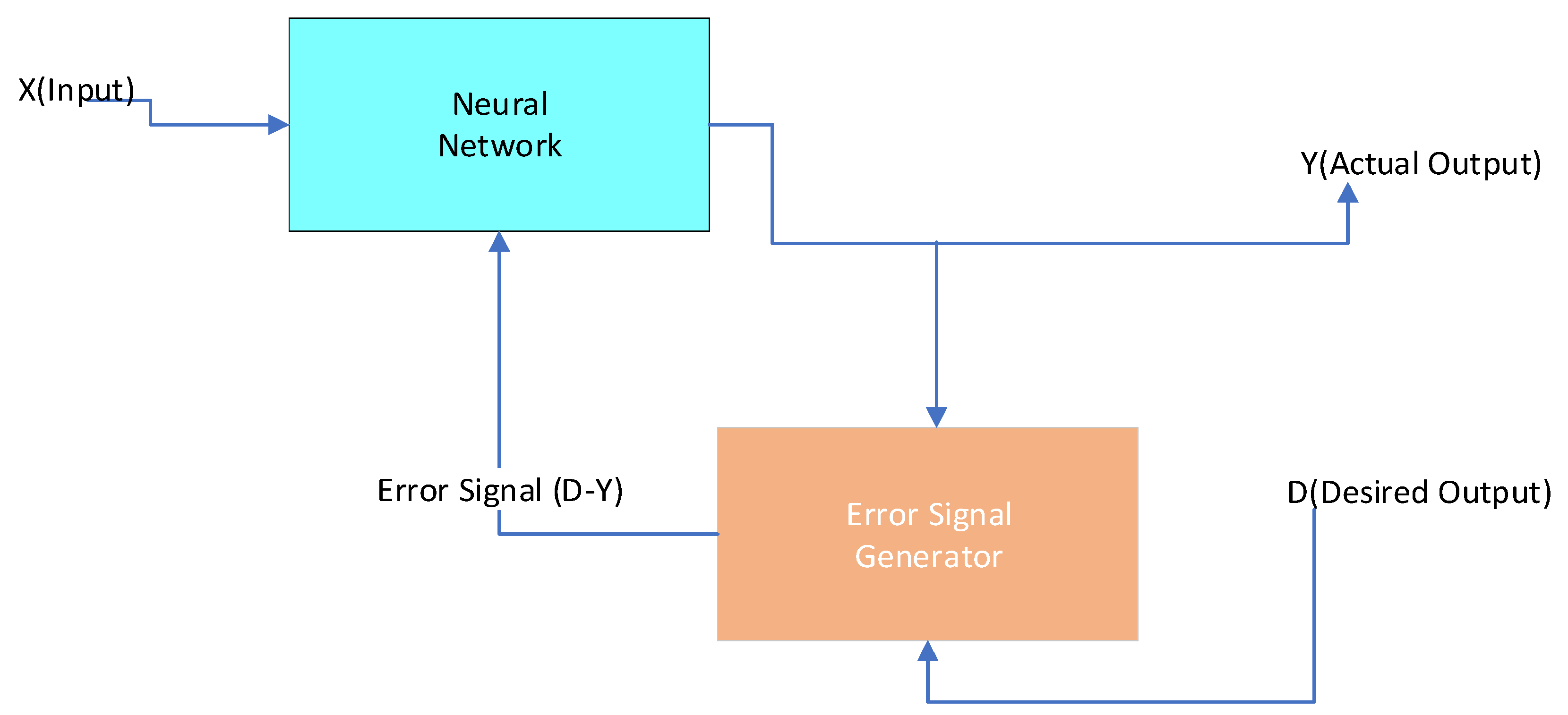
2.1.1. Artificial Neural Network

The architecture of Artificial Neural Network (ANN) as shown in Figure 1 is promptly the emerging zone of investigation, producing attention of predictors from a noble type of scientific field, which gives a deviation of desired output and actual output as an error signal. An error signal acts like a feedback to the neural network, which balances the desired and actual output.

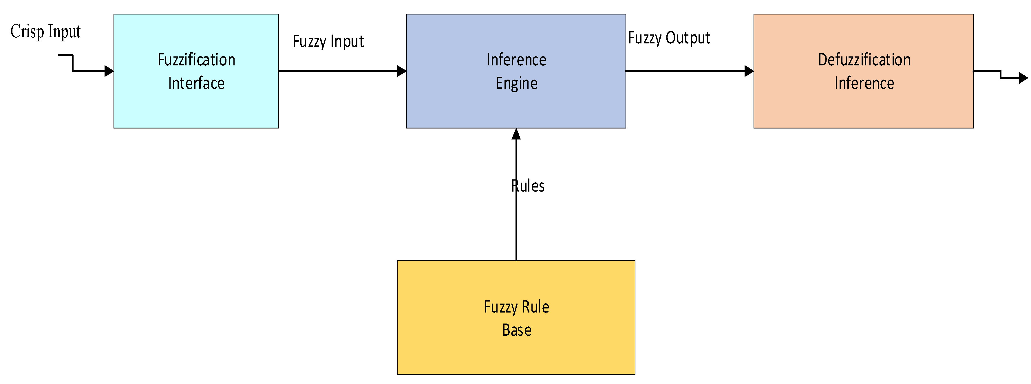
2.1.2. Fuzzy Logic Technique

The essential configuration of the scientific reasoning scheme in which the fuzzification [14] boundary recreates the additional contribution into a fuzzy verbal input, and likewise shows an significant character in the mathematical coherent [15] procedure as actual principles, which are delivered from current sensors, are a forever crisp analytical equivalent as shown in Figure 2.

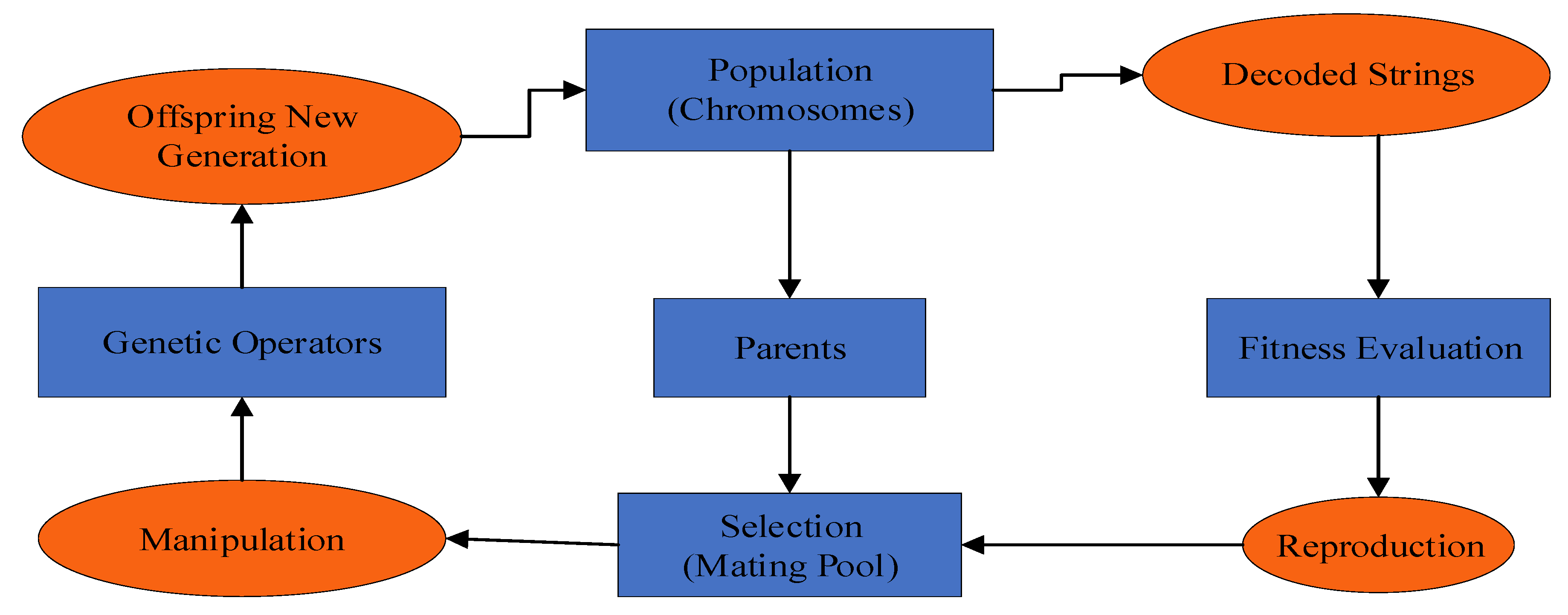
2.1.3. Genetic Algorithm

The overall thoughts were conceived by a European country [16], whereas practicality of persecution of exhausting it to untie innovative concerns was indisputable. It may be a soft computing style, which implements strategies stimulated by usual hereditary knowledge to develop conclusions to matters [17]. Genetic Algorithm (GA) as shown in Figure 3 is refreshed by Darwin’s theory concerning progression, which is useful to a vast variety of methodical and industrial problems like optimization, machine learning, and automatic software design [18].

2.2. Modern Intelligence Techniques

To solve the multi-disciplinary optimization problems [14], various modern practices are established by the investigators. The modern intelligence techniques are explored in the following sub-sections.

2.2.1. Differential Evolution Technique

It is a genetic-based algorithm [19] having identical operators corresponding to initialization, mutation, crossover, and selection. In this method, all constraints are expressive in genetic measurable by a genuine measurement [20]. The mathematical formulation of differential evolution is given below:

• Initialization

Firstly, whole vector of initial population is assigned any arbitrary assessment [21] starting with its equivalent state:

$$X_{j,i}^{\left(0\right)}=X_j^{min}+{\mu }_j\left( X_j^{max}-X_j^{min}\right),$$

(2)

where ${\mu }_j$ represents uniformly dispersed arbitrary numeral initialize with the array of [0, 1], generates novel for all value of $X_j^{min}$ and $X_j^{max}$ are representing the uppermost and lowermost limits of the j^th parameter, correspondingly.

• Mutation

This operator [22] generates distorted vectors $X_i^{\prime }$ by disturbing a randomly chosen vector ‘X_a’ and dissimilarity randomly chosen vectors ‘X_b’ and ‘X_c’ as per the following equation:

$$X_i^{\prime \left(G\right)}=X_a^{\prime \left(G\right)}+a\left(X_b^{\left(G\right)}+X_c^{\left(G\right)}\right) i=1,\dots ..N P,$$

(3)

where ‘X_a’,‘X_b’, and ‘X_c’ represent the randomly selected vectors among set of population, and ‘$\alpha$’ represents the scaling constant of the algorithm parameter which is used to regulate the size of the mutation operator and find better results.

• Crossover

Crossover operations [23] create trial vectors $X_i^{″}$ with integration of the parameters of the distorted vectors $X_i^{\prime }$ with its objective or parent vectors x_i:

$$X_{j,i}^{″}\left(G\right)=\{\begin{array}{c} X_{j,i}^{\prime \left(G\right)} if p_j \le C_R or j=q \\ X_{j,i}^{\left(G\right)} otherwise \end{array},$$

(4)

where p_j represents consistently discrete unplanned integer [24] between the variety of 0 and 1 and generates an extra for every value of j. q represents the random selected indicator {1, ..., NP} of the trial vector [25] obtain one parameter as a distorted vector. C_R representing the crossover operation constant of algorithm parameters [26] that manage the variety of population and algorithm is run absent as of local minima [27].

• Selection

Selection operator [28] develops the population by choosing the trial and parent vectors (precursor) which presents a best fitness [29]:

$$X_i^{\left(G+1\right)}=\{\begin{array}{c} X_i^{″\left(G\right)} if f\left( X_i^{″\left(G\right)}\right)\le f\left(X_i^{\prime \left(G\right)}\right) \\ X_i^{\left(G\right)} otherwise \end{array}i=1,\dots \dots ,NP.$$

(5)

This optimization procedure is replicate to the number of generations to obtain superior fitness functions because they required optimal values to explore the search space.

2.2.2. Biogeography Based Optimization

Biogeography Based Optimization (BBO) is the investigation of topographical propagation of living classes which is based on mutation and migration procedures [30].

• Migration

The migration process is either leaving or entering the species from an island. Biogeography-based optimization also used a population of candidate solution for optimization similar to partial swarm optimization and another population-based search method [31]. Depiction of all candidate solutions is complete as a vector of actual statistics. Now, all real statistics is considered in the population as suitability index variable (SIV). SIV [32] is similar to the output power of generating components in load frequency control. Few best solutions are the same in the resultant iterations; the migration process arranges to avoid the best solutions from being changed. Emigration rate [33] and immigration rate [34] for habitat contain ‘k’ species is express as:

$${\lambda }_k=I\left(1-\frac{K}{\eta }\right),$$

(6)

$${\mu }_k=\frac{Ek}{\eta },$$

(7)

where E represents the emigration rates, I represents the maximum immigration rates, and η represents the maximum number of species, respectively.

• Mutation

The habitat suitability index (HSI) [35] can easily be modified with resultant in the breed calculation to be different from the symmetry value, if a number of catastrophic actions occur. In biogeography-based optimization, this procedure is modeled as SIV mutation and the mutation rates of habitats may be intended to use the species add up probabilities known unexpected modification in weather of one habitat or additional occurrence will cause the unexpected modification in HSI (habitat). This condition is replica in the form of unexpected modification in the value of the suitability index variable in BBO. The probability of some organism [36] is calculated by this equation:

$$P_S=\{\begin{array}{c}-({\lambda }_S+{\mu }_S)P_S+{\mu }_{S+1}{P}_{S+1} S=0\\ -({\lambda }_S+{\mu }_S)P_S+{\lambda }_{S-1}{P}_{S-1}+{\mu }_{S+1}{P}_{S+1} 1\le S\le S_{max-1}\\ -({\lambda }_S+{\mu }_S)P_S+{\lambda }_{S-1}{P}_{S-1} S=S_{max}\end{array}.$$

(8)

The own probability of all members is one habitat. If probability of this is too low, and after that, this result has more probability to mutilation [37]. In a similar way, if the probability of a result is more, that result has a small probability to mutate. As a result, solutions with a low suitability index variable and high suitability index variable have a small possibility to grow an improved SIV in the new iteration. Dissimilar low suitability index variable and high suitability index [38] variable solutions, middle HSI solutions have a bigger possibility to grow improved solutions after the mutation process. By the use of equation mutation, all results can be calculated easily:

$$m\left(s\right)=m_{max}\left(\frac{1-P_S}{P_{max}}\right),$$

(9)

where m(s) represent the mutation rate.

2.2.3. Dragonfly Algorithm (DA)

DA [39] is an exceptional optimization process planned by Seyedali. The most important purpose of swarm is durability; thus, all individual must be unfocused outward, and opponents attracted towards nourishment sources. Taking both behaviors in swarms [40], these are five major topographies in position informing procedure of individuals. The numerical model of swarms actions as shown below: The parting procedure [41] in DA informing as in the above equation:

$$S_i=-{\displaystyle \sum }_{J=1}^{N}X-X_J,$$

(10)

where N represents the amount of entities of neighboring, X represents the present situation of specific, $X_J$ indicates the location of J^th specific of the adjacent [42].

The orientation procedure in this approach can be rationalized by subsequent expression [43]:

$$A_i=\frac{{{\displaystyle \sum }}_{J=1}^N{V}_J}{N},$$

(11)

where $V_J$ represents velocity of J^th specific of the adjacent. The unity in DA can be intended by the above evaluation:

$$C_i=\frac{{{\displaystyle \sum }}_{J=1}^N{X}_J}{N}-X,$$

(12)

where X represents the existing specific point, $X_J$ is the spot of J^th specific of the adjacent, and N indicates the amount of areas.

2.3. Hybrid Artificial Intelligence Techniques

2.3.1. Particle Swarm Optimization (PSO) and Gravitational Search Algorithm (GSA) Hybridization

The easiest technique to mongrelize PSO and GSA is to implement the strength separately in the successive approach [44].

Particle Swarm Optimization (PSO)

PSO is provoked with keen collective activities [45] accessible by a multiplicity of creatures, such as the group of ants or net of birds. The particle position and velocity both are updated according to the equations:

$$v_i^d\left(t+1\right)=w\left(t\right)v_i^d\left(t\right)+c_{1}X{r}_{1}X\left(pbes{t}_i^d-x_i^d\right)+c_2+r_2,$$

(13)

$$x_i^d\left(t+1\right)=x_i^d\left(t+1\right)+v_i^d\left(t+1\right),$$

(14)

$$Wt=rand X\frac{t}{t_{max}}X(w_{max}-w_{min})+w_{min},$$

(15)

where $v_i^d\left(t+1\right)$ shows velocity of (d^th) dimension at (t) reiteration of (i^th) particle, $x_i^d\left(t+1\right)$ is existing position of (d^th) dimensional iteration (t) of (i^th) particle; c₁ and c₂ representing the acceleration coefficients [46] which manage the pressure of gbest and pbest on the search procedure, r₁ and r₂ representing the arbitrary statistics in variety [0, 1]; $pbes{t}_i^d$ represents finest point of (i^th) element up to now.

Gravitational Search Algorithm (GSA)

GSA is meta-heuristic population-centered approach inspired with directions of attraction and quantity associations [47,48,49]. In this method, cause is dignified as article encompasses of unlike multitudes and the enactment of this is considered via crowds.

2.3.2. Differential Evolution and Particle Swarm Optimization Hybrids

It is a population-based optimizer [50] alike the genetic algorithm, having identical operatives corresponding to selection, mutation, and crossover. In this method, all constraints are expressive in genetic measurable by a genuine measurement [20,51].

2.3.3. Binary Moth Flame Optimizer (BMFO1)

BMFO is a newly projected meta-heuristics search algorithm proposed by Seyedali Mirjalili [52,53] which is refreshed by direction-finding behavior of moth and its converges near light. Although, moths are having a robust capability to uphold a secure approach with respect to the moon and hold a tolerable erection for nomadic in an orthodox mark for extensive distances. Besides, they are attentive in a fatal/idle curved track over simulated basis of lights.

2.3.4. Modified SIGMOID Transformation (BMFO2)

The binary calibration of constant pursuit house and places of search representatives, resolutions to binary exploration house could be the obligatory method for optimization of binary environmental issues such as LFC. In the proposed research, a modified sigmoidal transfer function is adopted, which has superior performance than another alternatives of sigmoidal transfer function as reported in [54].

2.3.5. Harris Hawks Optimizer

HHO [55] is gradient-free and populations-centered algorithm that comprises exploitative and exploratory stages, which is fortified by astonishment swoop, the fauna of examination of a victim, and diverse stratagems built on violent marvel of Harris hawks.

2.3.6. Smart Grid Applications

The modern smart grid system as shown in Figure 4 consists of various power generating units consisting of thermal, hydro, nuclear, wind, and solar-based power producing elements. The scheduling of every power producing in optimal condition is a tedious task and requires proper commitment schedule of generating units. Further, consideration of solar and wind-based energy sources requires proper load frequency control [56].

An electric grid can easily be converted into a smart grid by balancing the voltage, current, and frequency which is possible by the load frequency control method [57]. If incoming voltage, current, and frequency is matched with the outgoing voltage, current, and frequency of an electric grid with the help of optimal gain scheduling and load frequency control approach, then steady state error will be near to zero or nil. In the proposed research, load frequency control is tested and validated with various standard benchmarks simultaneously and mathematically depicted in the following sub-sections.

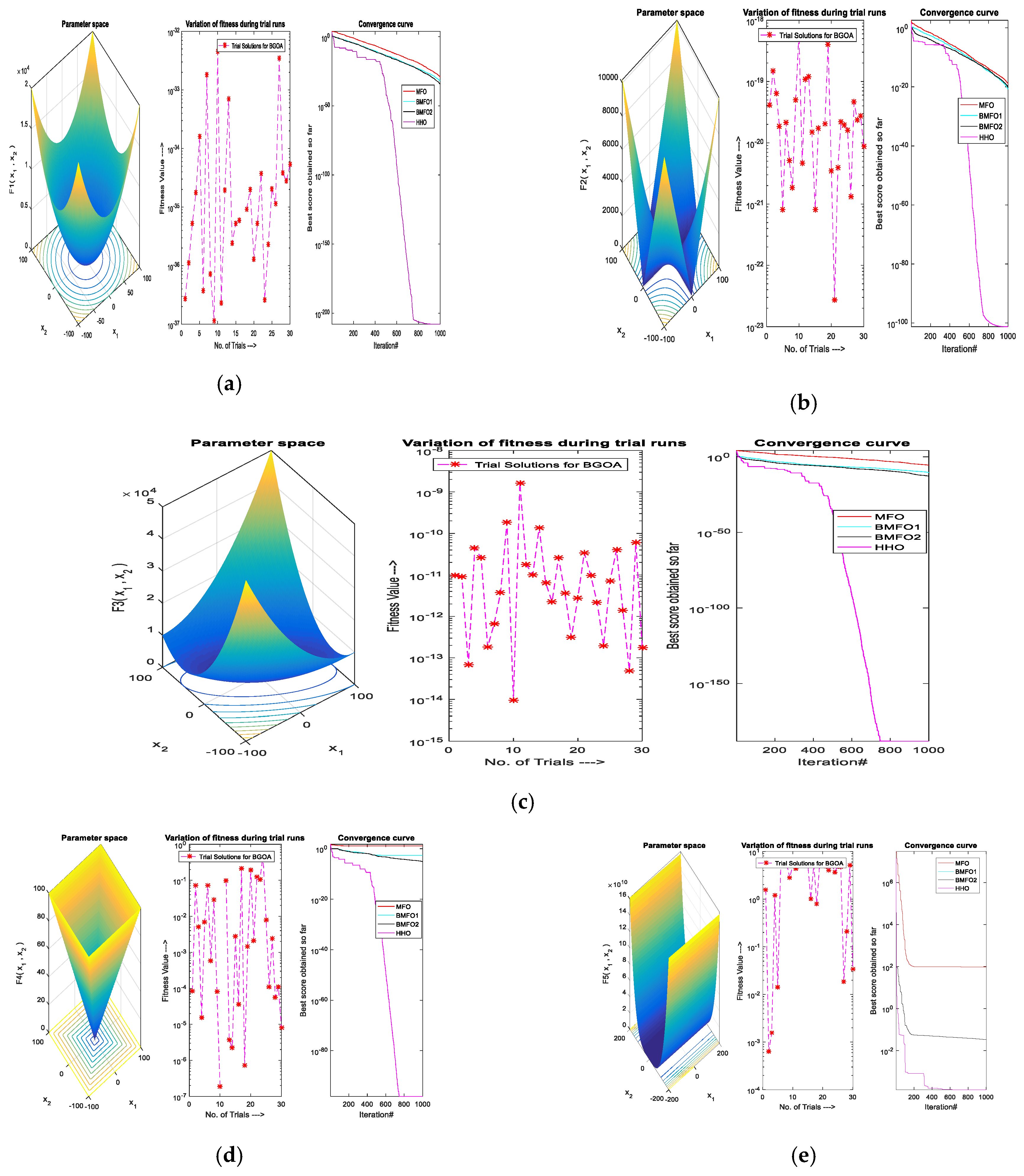
3. Standard Testing Benchmarks

The consequences for various benchmark issues [58] considering the LFC situation are deliberated in the above-mentioned units.

Test System and Standard Benchmark

For confirmation of prospects of deliberate BMFO and HHO algorithms, CEC2005 benchmark functions [59] have been taken into thought, which include unimodal, multi-modal, and fixed dimensions benchmark issues and its mathematical formulation has been represented in

Table 1. Unimodal benchmark.

Function	Dim	Range	${\mathit{f}}_{\mathbf{min}}$
$f_1\left(x\right)={\displaystyle {\displaystyle \sum }_{i=1}^n}{x}_i^2$	30	[−100, 100]	0
$f_2\left(x\right)={\displaystyle {\displaystyle \sum }_{i=1}^n}\left|x_i\right|+{\displaystyle {\displaystyle \prod }_{i=1}^n}\left|x_i\right|$	30	[−10,10]	0
$f_3\left(x\right)={\displaystyle {\displaystyle \sum }_{i=1}^n}{({\displaystyle {\displaystyle \sum }_{j-1}^i}{x}_j)}^2$	30	[−100, 100]	0
$f_4\left(x\right)=ma{x}_i\left\{\left|x_i\right|,1\le i\le n\right\}$	30	[−100, 100]	0
$f_5\left(x\right)={\displaystyle {\displaystyle \sum }_{i=1}^{n-1}}\left[100{\left(x_{i+1}-x_i^2\right)}^2+{\left(x_i-1\right)}^2\right]$	30	[−30, 30]	0
$f_6\left(x\right)={\displaystyle {\displaystyle \sum }_{i=1}^n}{\left(\left[x_i+0.5\right]\right)}^2$	30	[−100, 100]	0
$f_7\left(x\right)={\displaystyle {\displaystyle \sum }_{i=1}^n}i{x}_i^4$+ random $\left[0, 1\right]$	30	[−1.28, 1.28]	0

,

Table 2. Multimodal benchmark.

Function	Dim	Range	${\mathit{f}}_{\mathbf{min}}$
$f_8\left(x\right)={\displaystyle {\displaystyle \sum }_{i=1}^n}-x_i\sin (\sqrt{\left|x_i\right|})$	30	[−500, 500]	−418.98
$f_9\left(x\right)={\displaystyle {\displaystyle \sum }_{i=1}^n}\left[x_i^2-10 cos(2\Pi x_i)+10\right]$	30	[−5.12, 5.12]	0
$f_{10}\left(x\right)=-20\exp (-0.2\sqrt{\frac{1}{n}}{\displaystyle {\displaystyle \sum }_{i=1}^n}{x}_i^2)-\exp (\frac{1}{n}{\displaystyle {\displaystyle \sum }_{i=1}^n}\cos {\left(2\Pi x\right)}_i+20+c$	30	[−32, 32]	0
$f_{11}\left(x\right)=\frac{1}{4000}{\displaystyle {\displaystyle \sum }_{i=1}^n}{x}_i^2-{\displaystyle {\displaystyle \prod }_{i=1}^n}\cos (\frac{x_i}{\sqrt{i}}$) + 1	30	[−600, 600]	0
$f_{12}\left(x\right)=\frac{\Pi }{n}\left\{10\sin \left(\Pi y_1\right)+{\displaystyle {\displaystyle \sum }_{i=1}^{n-1}}{(y_i-1)}^2\left[1+10si{n}^2\left(\Pi y_{i+1}\right)+{(y_n-1)}^2\right]\right\}+{\displaystyle {\displaystyle \sum }_{i=1}^n}u(x_i,10,100,4)$ where $y_i=1+\frac{x_{i^{+1}}}{4}$ u($x_i,a,k,m)=\{\begin{array}{cc}k{(x_i-a)}^m,\hfill & x_i>a\hfill \\ 0,\hfill & -a<x_i<a\hfill \\ k{(-x_i-a)}^m\hfill & x_i<-a\hfill \end{array}$	30	[−50, 50]	0
$f_{13}\left(x\right)=0.1\{si{n}^2\left(3\Pi x_i\right)+{\displaystyle {\displaystyle \sum }_{i=1}^n}{\left(x_i-1\right)}^2\left[1+si{n}^2(3\Pi x_i+1\right]+{(x_m-1)}^2\left[1+si{n}^2\left(2\Pi x_m\right)\right]\}+{\displaystyle {\displaystyle \sum }_{i=1}^n}u(x_i$,5,100,4)	30	[−50, 50]	0
$f_{14}\left(x\right)=-{\displaystyle {\displaystyle \sum }_{i=1}^n}\sin (x_i).{\left(\sin \left(\frac{{ix}_i^2}{\Pi }\right)\right)}^{2m},m=10$	30	[0, π]	−4.687
$f_{15}\left(x\right)=\left[e-{\displaystyle {\displaystyle \sum }_{i=1}^n}{(x_i/\beta )}^{2m}-2e-{\displaystyle {\displaystyle \sum }_{i=1}^n}{x}_i^2\right]-{\displaystyle {\displaystyle \prod }_{i=1}^n}co{s}^2{x}_i,m=5$	30	[−20, 20]	−1
$f_{16}\left(x\right)=\left\{{\displaystyle {\displaystyle \sum }_{i=1}^n}si{n}^2\left(x_i\right)-exp\left(-{\displaystyle {\displaystyle \sum }_{i=1}^n}{x}_i^2\right)\right\}.exp\left[-{\displaystyle {\displaystyle \sum }_{i=1}^n}si{n}^2\sqrt{\left|x_i\right|}\right]$	30	[−10, 10]	−1

and

Table 3. Fixed dimension benchmark.

Function	Dim	Range	${\mathit{f}}_{\mathbf{min}}$
$f_{14}\left(x\right)={\left(\frac{1}{500}+{\displaystyle {\displaystyle \sum }_{j=1}^{25}}\frac{1}{ j+{{\displaystyle \sum }}_{i=1}^2{\left(x_i-a_{ij}\right)}^6}\right)}^{-1}$	2	[−65, 65]	1
$f_{15}\left(x\right)={\displaystyle {\displaystyle \sum }_{i=11}^{11}}{\left[a_i-\frac{x_i\left(b_i^2+b_i{x}_2\right)}{b_i^2+b_i{x}_3+x_4}\right]}^2$	4	[−5, 5]	0.00030
$f_{16}\left(x\right)=4x_1^2-2.1x_1^4+\frac{1}{3}{x}_1^6+x_1{x}_2-4x_2^2+4x_2^4$	2	[−5, 5]	−1.0316
$f_{17}\left(x\right)={\left(x_2-\frac{5.1}{4{\Pi }^2}{x}_1^2+\frac{5}{\Pi }{x}_1-6\right)}^2+10\left(1-\frac{1}{8\Pi }\right)cos{x}_i+10$	2	[−5, 5]	0.398
$f_{18}\left(x\right)=\left[1+{\left(x_1+x_2+1\right)}^2\left(19-14x_1+3x_1^2-14x_2+6x_1{x}_2+3x_2^2\right)\right] X \left[30+{\left(2x_1-3x_2\right)}^{2}X \left(18-32x_1+12x_1^2+48x_2-36x_1{x}_2+27x_2^2\right)\right]$	2	[−2, 2]	3
$f_{19}\left(x\right)=-{\displaystyle {\displaystyle \sum }_{i=1}^4}{c}_{i}exp\left(-{\displaystyle {\displaystyle \sum }_{j=1}^3}{a}_{ij}{\left(x_j-p_{ij}\right)}^2\right)$	3	[1, 3]	−3.32
$f_{20}\left(x\right)=-{\displaystyle {\displaystyle \sum }_{i=1}^4}{c}_{i}exp\left(-{\displaystyle {\displaystyle \sum }_{j=1}^6}{a}_{ij}{\left(x_j-p_{ij}\right)}^2\right)$	6	[0, 1]	−3.32
$f_{21}\left(x\right)=-{\displaystyle {\displaystyle \sum }_{i=1}^5}{\left[\left(x-a_i\right){\left(x-a_i\right)}^T+c_i\right]}^{-1}$	4	[0, 10]	−10.1532
$f_{22}\left(x\right)=-{\displaystyle {\displaystyle \sum }_{i=1}^7}{\left[\left(x-a_i\right){\left(x-a_i\right)}^T+c_i\right]}^{-1}$	4	[0, 10]	−10.4028
$f_{23}\left(x\right)=-{\displaystyle {\displaystyle \sum }_{i=1}^{10}}{\left[\left(x-a_i\right){\left(x-a_i\right)}^T+c_i\right]}^{-1}$	4	[0, 10]	−10.5363

. Table 1 interprets unimodal standard performance, Table 2 portrays multi-modal standard, and Table 3 interprets fixed dimensions standard issues.

To explain the random behavior of the expected BMFO2 logarithmic rule and confirm the consequences, thirty trials were applied with all objective function check for average, variance, best and worst values for justification of output from the probable algorithmic rule, unimodal benchmark work f1, f2, f3, f4, f5, f6, and f7 are used.

Table 4. (a) Outcomes of the BMFO1 algorithm. (b) Outcomes of the BMFO2 algorithm. (c) Outcomes of the HHO algorithm.

Benchmark Functions	Parameters
	Mean Value	SD	Worst Value	Best Value	p-Value
(a)
f1	5.75 × 10−34	2.55 × 10−33	1.40 × 10−32	0	3.79 × 10−060
f2	1.48 × 10−20	2.24 × 10−20	1.14 × 10−19	0	3.79 × 10−060
f3	3.87 × 10−10	1.61 × 10−09	8.70 × 10−09	0	2.56 × 10−060
f4	0.03831	0.08819	0.4401	0	2.56 × 10−060
f5	3.14461	2.21914	6.01278	0	2.56 × 10−060
f6	1.27 × 1032	1.60 × 10−32	8.32 × 10−32	0	7.23 × 10−060
f7	1.00564	1.00438	1.01652	0	1.74 × 10−060
(b)
f1	3.64 × 10−34	1.05 × 10−33	4.50 × 10−33	0	2.56 × 10−060
f2	6.08 × 10−20	1.30 × 10−19	6.12 × 10−19	0	2.56 × 10−060
f3	7.64 × 10−11	3.00 × 10−10	1.65 × 10−09	9.46 × 10−15	1.73 × 10−060
f4	0.04709	0.09997	0.47495	0	2.56 × 10−060
f5	3.4591	2.2489	6.2531	0.00064	1.73 × 10−060
f6	2.85 × 10−32	5.78 × 10−32	3.08 × 10−31	0	1.61 × 10−050
f7	1.00499	1.00387	1.01831	0.00032	1.74 × 10−060
(c)
f1	1.0634 × 10−90	5.82468 × 10−90	3.19 × 10−89	8.7 × 10−112	1.734 × 10−06
f2	6.9187 × 10−51	2.46844 × 10−50	1.31 × 10−49	1.71 × 10−60	1.734 × 10−06
f3	1.251 × 10−80	6.62663 × 10−80	3.632 × 10−79	8.3 × 10−99	1.734 × 10−06
f4	4.4615 × 10−48	1.70307 × 10−47	8.676 × 10−47	2.45 × 10−59	1.734 × 10−06
f5	0.01500185	0.023472777	0.0874276	1 × 10−05	1.734 × 10−06
f6	0.00011487	0.00015409	0.0007119	4.17 × 10−07	1.734 × 10−06
f7	0.00015829	0.000224928	0.001202	2.87 × 10−06	1.734 × 10−06

(a) signifies the response of unimodal benchmark function with BMFO1 logarithmic rule, Table 4 (b) characterizes the retort of unimodal benchmark operate function by using the BMFO2 algorithmic rule and Table 4 (c) represents the answer of the fixed dimension benchmark function by using HHO algorithmic instruction.

It is analyzed from Table 4 that the unimodel benchmark functions f1 to f7 are tested using the modern hybrid algorithms like BMFO 1, BMFO 2, and HHO, and found that Harris hawks optimizer (HHO) produces optimal outcomes in terms of mean, standard deviation, best and worst value for all functions as compared to other algorithms. The convergence curve and trial solutions for BMFO1, BMFO2, and HHO for f1 to f7 unimodal benchmark functions are presented in Figure 5.

The convergence curve and trial solutions for BMFO1, BMFO2, and HHO for f1 to f7 unimodal benchmark functions are presented in Figure 5a–g.

The connected upshots for unimodal standard functions [60] have been represented in

Table 5. Comparison of unimodal benchmark functions.

Algorithm	Parameter	Uni-Modal Benchmark Functions
		f1	f2	f3	f4	f5	f6	f7
GWO [62]	Mean	0.02	0	0.01	1.02	26.81	0.82	0
	SD	0	0.03	79.15	1.32	69.9	0	0.1
PSO [63,64]	Mean	0	0.04	70.13	1.09	96.72	0	0.12
	SD	0	0.05	22.12	0.32	60.12	0	0.04
GSA [8,65]	Mean	0	0.06	896.53	7.35	67.54	0	0.09
	SD	0	0.19	318.96	1.74	62.23	0	0.04
DE [66,67]	Mean	0.01	0.01	0.01	0.01	0.01	0.01	0.01
	SD	1.01	1.01	1.01	1.01	1.01	1.01	1.01
FOA [68,69]	Mean	0.05	0.06	0.04	0.4	5.06	0.02	0.14
	SD	0.02	0.02	0.01	1.5	5.87	0	0.35
ALO [70,71]	Mean	0.01	0.01	0	0.01	0.35	0.01	0
	SD	0.01	0	0.01	0.01	0.11	0.01	0.01
SOS [72]	Mean	0.06	0.01	0.96	0.28	0.09	0.13	0
	SD	0.01	0	0.82	0.01	0.14	0.08	0
BA [73]	Mean	1.77	1.33	1.12	1.19	1.33	1.78	1.14
	SD	1.53	4.82	1.77	1.89	1.3	1.67	1.11
FPA [74,75]	Mean	0.01	0.01	0.01	0.01	0.78	0.01	0.01
	SD	0.01	0.01	0.01	0.01	0.37	0.01	0.01
CS [76]	Mean	0	1.21	1.25	0.01	0.01	0.01	0.01
	SD	0	1.04	1.02	0.01	0.01	0.01	0.01
FA [52]	Mean	0.04	0.05	0.05	0.15	2.18	0.06	0
	SD	0.01	0.01	0.02	0.03	1.45	0.01	0
GA [77]	Mean	0.12	0.15	0.14	0.16	0.71	0.17	0.01
	SD	0.13	0.05	0.12	0.86	0.97	0.87	0
GOA [73,78]	Mean	0.01	0.01	0.01	0.01	0.01	0.01	0.01
	SD	0.01	0.01	0.02	0.01	0.01	0.01	0.01
MFO [79]	Mean	0.01	0.01	0.01	0.07	27.87	3.12	0
	SD	0	0	0	0.4	0.76	0.53	0
MVO [80]	Mean	2.09	15.92	453.2	3.12	1272.1	2.29	0.05
	SD	0.65	44.75	177.1	1.58	1479.5	0.63	0.03
DA [81]	Mean	0.01	0.01	0.01	0.01	7.6	0.01	0.01
	SD	0.01	0.01	0.01	0.01	6.79	0.01	0.01
BBA [65]	Mean	1.28	1.06	15.6	1.25	24.7	1.1	1.01
	SD	1.42	1.07	23.8	1.33	35.8	1.14	1.01
BBO [5,82]	Mean	6.52	0.2	16.7	2.8	87.6	7.96	0.01
	SD	2.99	0.05	14.9	1.47	66.9	4.87	0.01
BGSA [83,84]	Mean	85	1.19	458	7.35	3110	109	0.04
	SD	48.7	0.23	275	2.25	2936	77.7	0.06
SCA [85,86]	Mean	0.01	0.01	0.06	0.1	0.01	0.01	0.01
	SD	0.01	0.01	0.14	0.58	0.01	0.01	0.01
SSA [88]	Mean	0.01	0.23	0.01	0.01	0.01	0.01	0.01
	SD	0.01	1	0.01	0.66	0.01	0.01	0.01
WOA [89]	Mean	0.01	0.01	696.73	70.69	139.15	0.01	0.09
	SD	0.01	0.01	188.53	5.28	120.26	0.01	0.05
BMFO1	Mean	0.01	0.01	0.01	0.04	3.14	0.01	0.01
	SD	0.01	0.01	0.01	0.09	2.22	0.01	0.01
BMFO2	Mean	0.01	0.01	0.01	0.05	3.46	0.01	0.01
	SD	0.01	0.01	0.01	0.1	2.25	0.01	0.01
HHO (Proposed)	Mean	1.06 × 10−90	6.92 × 10−51	1.25 × 10−80	4.46 × 10−48	0.015002	0.000115	0.000158
	SD	5.82 × 10−90	2.47 × 10−50	6.63 × 10−80	1.70 × 10−47	0.023473	0.000154	0.000225

, which are correlated with various latest refined algorithms [61] grey wolf optimizer (GWO) [62], PSO [63,64], GSA [8,65], differential evolution (DE) [66,67], fruit fly optimization algorithm (FOA) [68,69], ant lion optimizer (ALO) [70,71], symbiotic organisms search (SOS) [72], bat algorithm (BA) [73], flower pollination algorithm (FPA) [74,75], cuckoo search (CS) [76], firefly algorithm (FA) [52], GA [77], grasshopper optimization algorithm (GOA) [73,78], MFO [79], multiverse optimization algorithm (MVO) [80], DA [81], binary bat optimization algorithm (BBA) [65], BBO [5,82], binary gravitational search algorithm (BGSA) [83,84], sine cosine algorithm (SCA) [85,86], FPA [74,87], salp swarm optimization algorithm (SSA) [88], and whale optimization algorithm (WOA) [89] in lieu of mean and standard deviation.

To defend the synthesis part of the probable algorithm, multi-modal benchmark functions f8, f9, f10, f11, f12, and f13 are taken with numerous native goals with values rising violently w.r.t magnitude.

Table 6. (a) Outcomes of the BMFO1 algorithm. (b) Outcomes of the BMFO2 algorithm. (c) Results of the HHO algorithm.

Benchmark Functions	Parameters
	Mean Value	SD	Worst Value	Best Value	p-Value
(a)
f8	−3140.3	290.75	−2641	−4071.4	0
f9	1.63	0.96	2.98	0.01	0
f10	0.04	0.21	1.16	0.01	0
f11	0.01	0.01	0.01	0.01	1
f12	0.01	0.01	0.01	0.01	0.01
f13	0	0	0.01	0	0
(b)
f8	−3361.2	287.325	−2879.4	−4071.4	1.73 × 10−06
f9	1.39294	0.72032	2.98488	0	3.89 × 10−06
f10	4.56 × 10−15	0	4.56 × 10−15	4.56 × 10−15	4.33 × 10−08
f11	0	0	0	0	1
f12	4.82 × 10−32	8.59 × 10−34	5.12 × 10−32	4.71 × 10−32	1.56 × 10−06
f13	0.00256	0.01025	0.05478	1.35 × 10−32	1.34 × 10−06
(c)
f8	−12561.4	40.82419124	−12345.3	−12569.5	1.7344 × 10−06
f9	0.01	0.01	0.01	0.01	1
f10	8.88 × 10−161	0.01	8.88 × 10−161	8.88 × 10−161	4.3205 × 10−08
f11	0.01	0.01	0.01	0.01	1
f12	8.92 × 10−06	1.16218 × 10−05	4.76 × 10−05	4.64 × 10−08	1.7344 × 10−06
f13	0.000101	0.000132197	0.000612	7.35 × 10−07	1.7344 × 10−06

(a) presents clarification of the multimodal benchmark function with the BMFO1 algorithm and Table 6 (b) presents the explanation of the multimodal benchmark function with the BMFO2 algorithm and Table 6 (c) presents the explanation of the multimodal benchmark function with the HHO algorithm.

It is analyzed from Table 6 that multi-model benchmark functions f8 to f13 are tested using modern hybrid algorithms like BMFO 1, BMFO 2, and HHO and found that the Harris hawks optimizer (HHO) produces optimal outcomes in terms of mean, standard deviation, best and worst value for all functions as compared to other algorithms.

The convergence curve and trial solutions for BMFO1, BMFO2, and HHO for f8 to f13 multi-modal benchmark functions are presented in Figure 6a–f.

The connected outcomes for multimodal benchmark functions has been signified in

Table 7. Comparison of multi-modal benchmark functions.

Algorithms	Parameters	Multi-Modal Benchmark Functions
		f8	f9	f10	f11	f12	f13
GWO [62]	Mean	−6120	0.31	0	0	0.05	0.65
	SD	−4090	47.4	0.08	0.01	0.02	0
PSO [63,64]	Mean	−4840	46.7	0.28	0.01	0.01	0.01
	SD	1150	11.6	0.51	0.01	0.03	0.01
GSA [8,65]	Mean	−2820	26	0.06	27.7	1.8	8.9
	SD	493	7.47	0.24	5.04	0.95	7.13
DE [66,67]	Mean	−11100	69.2	0	0	0	0
	SD	575	38.8	0	0	0	0
FOA [68,69]	Mean	−12600	0.05	0.02	0.02	0	0
	SD	52.6	0.01	0	0.02	0	0
ALO [70,71]	Mean	−1610	0	0	0.02	0	0
	SD	314	0	0	0.01	0	0
SOS [72]	Mean	−4.21	1.33	0	0.71	0.12	0.01
	SD	0	0.33	0	0.91	0.04	0
BA [73]	Mean	−1070	1.23	0.13	1.45	0.4	0.39
	SD	858	0.69	0.04	0.57	0.99	0.12
FPA [74,75]	Mean	−1840	0.27	0.01	0.09	0	0
	SD	50.4	0.07	0.01	0.04	0	0
CS [76]	Mean	−2090	0.13	0	0.12	0	0
	SD	0.01	0	0	0.05	0	0
FA [52]	Mean	−1250	0.26	0.17	0.1	0.13	0
	SD	353	0.18	0.05	0.02	0.26	0
GA [77]	Mean	−2090	0.66	0.96	0.49	0.11	0.13
	SD	2.47	0.82	0.81	0.22	0	0.07
GOA [73,78]	Mean	1	0	0.1	0	0	0
	SD	0	0	1	0	0	0
MFO [79]	Mean	−5080	0	7.4	0	0.34	1.89
	SD	696	0	9.9	0	0.22	0.27
MVO [80]	Mean	−11700	118	4.07	0.94	2.46	0.22
	SD	937	39.3	5.5	0.06	0.79	0.09
DA [81]	Mean	−2860	16	0.23	0.19	0.03	0
	SD	384	9.48	0.49	0.07	0.1	0
BBA [65]	Mean	−924	1.81	0.39	0.19	0.15	0.04
	SD	65.7	1.05	0.57	0.11	0.45	0.06
BBO [5,82]	Mean	−989	4.83	2.15	0.48	0.41	0.31
	SD	16.7	1.55	0.54	0.13	0.23	0.24
BGSA [83,84]	Mean	−861	10.3	2.79	0.79	9.53	2220
	SD	80.6	3.73	1.19	0.25	6.51	5660
SCA [85,86]	Mean	1	0.01	0.38	0.01	0.01	0.01
	SD	0.01	0.73	1	0.01	0.01	0.01
SSA [88]	Mean	0.06	0.01	0.2	0.01	0.14	0.08
	SD	0.81	0.01	0.15	0.07	0.56	0.71
MFO [79]	Mean	−8500	84.6	1.26	0.02	0.89	0.12
	SD	726	16.2	0.73	0.02	0.88	0.19
BMFO1	Mean	−3140.3	1.63	0.04	0	0	0
	SD	290.75	0.96	0.21	0	0	0
BMFO2	Mean	−3361.2	1.39	0	0	0	0
	SD	287.32	0.72	0	0	0	0.01
HHO (Proposed)	Mean	−12561.38	0	8.88 × 10−16	0	8.92 × 10−06	0.000101
	SD	40.82419	0	0	0	1.16 × 10−05	0.000132

, which are associated with various latest refined meta-heuristics search algorithms like GWO [62], PSO [63,64], GSA [8,65], DE [66,67], FOA [68,69], ALO [70,71], SOS [72], BA [73], FPA [74,75], CS [76], FA [52], GA [77], GOA [73,78], MFO [79], MVO [80], DA [81], BBA [65], BBO [5,82], BGSA [83,84], SCA [85,86], FPA [74,87], SSA [88], and WOA [89] in lieu of average [90] and standard deviation.

The verified consequences for fixed dimension benchmark situations are obtainable in

Table 8. (a) Outcomes of the BMFO1 algorithm. (b) Outcomes of the BMFO2 algorithm. (c) Outcomes of the HHO algorithm.

Benchmark Functions	Parameters
	Mean Value	SD	Worst Value	Best Value	p-Value
(a)
f14	12.61	1.35	12.67	10.76	0
f15	0	0	0	0	0
f16	−1.03	0	−1.03	−1.03	0
f18	3	0	3	3	0
f19	−3.86	0	−3.85	−3.86	0
f20	−3.16	0.08	−2.86	−3.32	0
f21	−5.06	0	−5.06	−5.06	0
f22	−5.09	0	−5.09	−5.09	0
f23	−5.13	0	−5.13	−5.13	0
(b)
f14	12.67	0	12.67	12.67	0
f15	0	0	0	0	0
f16	−1.03	0	−1.03	−1.03	0
f18	3	0	3	3	0
f19	−3.86	0	−3.85	−3.86	0
f20	−3.17	0.12	−2.81	−3.32	0
f21	−5.06	0	−5.06	−5.06	0
f22	−5.09	0	−5.09	−5.09	0
f23	−5.13	0	−5.13	−5.13	0
(c)
f14	2.361171	1.95204	5.928845	1.998004	1.73 × 10−08
f15	1.00035	3.2 × 10−05	0.000433	0.000309	1.73 × 10−08
f16	−1.03162	2.86 × 10−09	−1.03162	−1.03162	1.73 × 10−08
f17	0.397895	1.6 × 10−05	0.397948	0.397887	1.73 × 10−06
f18	3.000001	4.94 × 10−06	3.000027	2	1.73 × 10−08
f19	−2.85977	1.005195	−3.8354	−3.86274	1.73 × 10−08
f20	−2.06481	0.136148	−2.74389	−3.26174	1.73 × 10−08
f21	−4.37397	1.227502	−5.0413	−10.0309	1.73 × 10−06
f22	−5.08346	0.004672	−5.06481	−5.08765	1.73 × 10−06
f23	−5.78398	1.712458	−5.1145	−10.3706	1.73 × 10−06

.

It is analyzed from Table 8 that fixed dimension benchmark functions f14 to f23 are tested using modern hybrid algorithms like BMFO 1, BMFO 2, and HHO and found that Harris hawks optimizer (HHO) produces optimal outcomes in terms of mean, standard deviation, best and worst value for all functions as compared to other algorithms.

The convergence curve and trial solutions for BMFO1, BMFO2, and HHO for f14 to f23 fixed dimension benchmark functions are presented in Figure 7a–j.

The comparative outcomes for fixed dimension benchmark [91] functions have been represented in

Table 9. Comparison of fixed dimension benchmark functions.

Algorithms	Parameters	Composite Benchmark Functions
		f14	f15	f16	f17	f18	f19
GWO [62]	Mean	3.06	0	−1.03	0.4	3	−3.86
	SD	4.25	0	−1.03	0.4	3	−3.86
PSO [63,64]	Mean	3.63	0	−1.03	0.4	3	−3.86
	SD	2.56	0	0	0	0	0
GSA [8,65]	Mean	5.86	0	−1.03	0.4	3	−3.86
	SD	3.83	0	0	0	0	0
DE [66,67]	Mean	1	0	−1.03	0.4	3	NA
	SD	0	0	0	0	0	NA
FOA [68,69]	Mean	1.22	0	−1.03	0.4	3.02	−3.86
	SD	0.56	0	0	0	0.11	0
ALO [70,71]	Mean	0	14.6	175	316	4.4	500
	SD	0	32.2	46.5	13	1.66	0.21
SOS [72]	Mean	776.48	873.8	961	899.86	741	900.5
	SD	0	9.72	67.2	0	0.79	0.84
BA [73]	Mean	182.48	487.2	588.2	756.98	542	818.5
	SD	117.02	161.4	137.8	160.1	220	152.5
FPA [74,75]	Mean	0.34	18.23	224	362.03	10.2	504
	SD	0.24	3.07	50.3	54.02	1.39	1.16
CS [76]	Mean	110	140.6	290	402	213	812
	SD	110.05	92.8	86.1	98.2	206	192
FA [52]	Mean	150.17	314.5	734.5	818.57	134	862.2
	SD	97.16	92.93	204	109.97	216	126
GA [77]	Mean	114.61	95.46	325.4	466.31	90.4	521.2
	SD	26.96	7.16	51.67	29.57	13.7	27.99
GOA [73,78]	Mean	0	0.49	0	0.82	0	0.79
	SD	0.34	0.72	0	1	0.01	0.94
MFO [79]	Mean	2.11	0	−1.03	0.4	3	−3.86
	SD	2.5	0	0	0	0	0
MVO [80]	Mean	10	30.01	50	190.3	161	440
	SD	31.62	48.31	52.7	128.67	158	51.64
DA [81]	Mean	104	193	458	596.66	230	680
	SD	91.2	80.6	165	171.06	185	199
BBA [65]	Mean	1.39	1.02	1.05	1	1.01	1
	SD	1.19	1.07	1.49	1.11	1.01	1.2
BBO [5,82]	Mean	0.06	0	0.2	0	0.14	0.08
	SD	0.81	0	0.15	0.07	0.56	0.71
MFO [79]	Mean	0	66.73	119	345.47	10.4	707
	SD	0	53.23	28.33	43.12	3.75	195
BMFO1	Mean	12.61	0	−1.03	0	3	−3.86
	SD	0.35	0	0	0	0	0
BMFO2	Mean	12.67	0	−1.03	0	3	−3.86
	SD	0	0	0	0	0	0
HHO (Proposed)	Mean	1.361171	0.00035	−1.03163	0.397895	3.000001225	−3.8597664
	SD	0.95204	3.20 × 10−05	1.86 × 10−09	1.60 × 10−05	4.94 × 10−06	0.00519467

and

Table 10. Comparison of results for fixed dimension functions.

Algorithms	Parameters	Benchmark Functions
		f20	f21	f22	f23
GWO [62]	Mean	−2.79	−9.8	−9.9	−9.69
	SD	−2.84	−9.18	−7.55	−7.48
PSO [63,64]	Mean	−2.29	−7.89	−7.49	−8.99
	SD	1.06	3.07	4.08	1.76
GSA [8,65]	Mean	−2.36	−4.99	−8.64	−10.63
	SD	1.02	4.74	2.01	0
DE [66,67]	Mean	0.01	−10.2	−10.4	−10.54
	SD	0.01	0	0	0
FPA [74,75]	Mean	−4.28	−6.56	−6.57	−7.59
	SD	0.08	1.57	2.18	3.18
WOA [84]	Mean	−2.98	−7.05	−8.18	−9.34
	SD	0.38	3.63	3.83	2.41
BMFO1	Mean	−3.16	−5.06	−5.09	−5.13
	SD	0.08	0	0	0
BMFO2	Mean	−3.17	−5.06	−5.09	−5.13
	SD	0.12	0	0	0
HHO (Proposed)	Mean	−3.06481	−5.37397	−5.08346	−5.78398
	SD	0.136148	1.227502	0.004672	1.712458

, which are associated with other latest refined met heuristics search algorithms [54,92] GWO [62], PSO [63,64], GSA [8,65], DE [66,67], FOA [68,69], ALO [70,71], SOS [72], BA [73], FPA [74,75], CS [76], FA [52], GA [77], GOA [73,78], MFO [79], MVO [80], DA [81], BBA [65], BBO [5,82], BGSA [83,84], SCA [85,86], FPA [74,87], SSA [88], and WOA [89] in terms of standard deviation [93] and average.

4. Conclusions

The smart grid process needs a continuing matching of resource and ultimatum in accordance with recognized functioning principles of numerous algorithms. The LFC scheme delivers the consistent action of power structure by constantly balancing the resource of electricity with the response, while also confirming the accessibility of adequate supply volume in upcoming periods. In this paper, binary variations of the moth flame optimizer and HHO have been analyzed and tested to solve twenty-three benchmark problems including unimodel, multi-model, and fixed dimension functions which investigate that the proposed Harris hawks optimizer approach suggestions are offering better results as associated to substitute labeled meta-heuristics search algorithms. In upcoming work, the effectiveness of the HHO technique is deliberate for optimal matching of total generation with total consumption of electrical energy to convert an electric grid to smart grid. So, by using the Harris hawks optimizer, we can easily balance the smart grid elements by matching production and consumption of electrical energy.

References

- García, J.; Martí, J.V.; Yepes, V. The Buttressed Walls Problem: An Application of a Hybrid Clustering Particle Swarm Optimization Algorithm. Mathematics 2020, 8, 862. [Google Scholar] [CrossRef]
- Ziegler, J.G.; Nichols, N.B. Optimum settings for automatic controllers. Trans. ASME 1942, 64, 759–768. [Google Scholar] [CrossRef]
- Elgerd, O.I.; Fosha, C.E. Optimum Megawatt-Frequency Control of Multiarea Electric Energy Systems. IEEE Trans. Power Appar. Syst. 1970, 89, 556–563. [Google Scholar] [CrossRef]
- Mamdani, E.H. Application of fuzzy algorithms for control of simple dynamic plant. Proc. IEEE 1974, 121, 1585–1588. [Google Scholar] [CrossRef]
- Du, D.; Simon, D.; Ergezer, M. Biogeography-Based Optimization Combined with Evolutionary Strategy and Immigration Refusal. In Proceedings of the IEEE Proc. International Conference on Systems, Man and Cybernetics, San Antonio, TX, USA, 11–14 October 2009; Volume 1, pp. 997–1002. [Google Scholar]
- Byerly, R.T.; Sherman, D.E.; Bennon, R.J. Frequency Domain Analysis of Low Frequency Oscillations in Large Electric Power Systems, Part-1, Basic Concepts, Mathematical Model and Computing Methods; 727, Project 744-1; EPRI-EL: Palo Alto, CA, USA, 1979; Volume 1, pp. 1–7. [Google Scholar]
- Meng, G.; Xiong, H.; Li, H. Power system load-frequency controller design based on discrete variable structure control theory. In Proceedings of the 2009 IEEE 6th International Power Electronics and Motion Control Conference, Wuhan, China, 17–20 May 2009; Volume 2, pp. 2591–2594. [Google Scholar]
- Rashedi, E.; Nezamabadi-Pour, H.; Saryazdi, S. GSA: A gravitational search algorithm. Inf. Sci. 2009, 179, 2232–2248. [Google Scholar] [CrossRef]
- Beaufays, F.; Magid, Y.A.; Widrow, B. Application of neural networks to load-frequency control in power systems. Neural Netw. 1994, 7, 183–194. [Google Scholar] [CrossRef]
- Kothari, M.L.; Kaul, B.L.; Nanda, J. Automatic generation control of hydro-thermal system. J. Inst. Eng. India 1980, 61, 85–91. [Google Scholar]
- Cohen, A.I.; Yoshimura, M. A Branch-and-Bound Algorithm for Unit Commitment. IEEE Trans. Power Appar. Syst 1983, 102, 444–451. [Google Scholar] [CrossRef]
- Pan, C.T.; Liaw, C.M. An adaptive controller for power system Load-frequency control. IEEE Trans. Power Syst. 1989, 4, 122–128. [Google Scholar] [CrossRef]
- Sugeno, M. An introductory survey of fuzzy control. Inf. Sci. 1985, 36, 59–83. [Google Scholar] [CrossRef]
- Birch, A.P.; Sapeluk, A.T.; Ozveren, C.S. An enhanced neural network load frequency control technique. In Proceedings of the Control ’94, Conference Publication, Coventry, UK, 21–24 March 1994; Volume 389, pp. 409–415. [Google Scholar]
- Bekhouche, N.; Feliachi, A. Decentralized estimation for the Automatic Generation Control problem in power systems. In Proceedings of the [Proceedings 1992] The First IEEE Conference on Control Applications, Dayton, OH, USA, 13–16 September 1992; Volume 3, pp. 621–632. [Google Scholar]
- Elgerd, O.J. Electric Energy Systems Theory: An Introduction; Tata Mcgraw Hill: New York, NY, USA, 1983. [Google Scholar]
- Kocaarsian, I.; Cam, E. Fuzzy Logic Controller in interconnected electrical power systems for Load Frequency Control. Electr. Power Energy Syst. 2005, 27, 542–549. [Google Scholar] [CrossRef]
- Holland, J.H. Adaptation in Natural and Artificial Systems: An Introductory Analysis; MIT Press: Cambridge, MA, USA, 1992. [Google Scholar]
- Wang, Y.; Zhou, R.; Wen, C. New robust adaptive load-frequency control with system parametric uncertainties. IEE Proc. Gener. Transm. Distrib. 1994, 141, 184–190. [Google Scholar] [CrossRef]
- Cohn, N. Techniques for improving the control of bulk power transfers on interconnected systems. IEEE Trans. Power Appar. Syst. 1971, 90, 2409–2419. [Google Scholar] [CrossRef]
- Oneal, A.R. A Simple Method for Improving Control Area Performance: Area Control Error (ACE) Diversity Interchange. IEEE Trans. Power Syst. 1995, 10, 1071–1076. [Google Scholar] [CrossRef]
- Kothari, D.P.; Ahmad, A. An expert system approach to the unit commitment problem. Energy Convers. Manag. 1995, 36, 257–261. [Google Scholar] [CrossRef]
- Hsu, S.-C.; Jane, Y.-J.H.S.U.; I-Jen, C. Automatic Generation of Fuzzy Control Rules by Machine Learning Methods. In Proceedings of the IEEE International Conference on Robotics and Automation, Nagoya, Japan, 21–27 May 1995; Volume 1, pp. 287–292. [Google Scholar]
- Indulkar, C.S.; Raj, B. Application of fuzzy controller to Automatic Generation Control. Electr. Mach. Power Syst. 1995, 23, 209–220. [Google Scholar] [CrossRef]
- Chang, C.S.; Fu, W. Area load frequency control using fuzzy gain scheduling of PI controllers. Electr. Power Syst. Res. 1997, 42, 145–152. [Google Scholar] [CrossRef]
- Kennedy, J.; Eberhart, R.C. A discrete binary version of the particle swarm algorithm. In Proceedings of the IEEE Conference on Systems, Man, and Cybernetics, Orlando, FL, USA, 12–15 October 1997; Volume 5, pp. 4104–4108. [Google Scholar]
- Kumar, J. AGC simulator for price-based operation-Part I: A Model. IEEE Trans. Power Syst. 1997, 12, 527–532. [Google Scholar] [CrossRef]
- Bakken, B.H.; Grande, O.S. Automatic Generation Control in a deregulated power system. IEEE Trans. Power Syst. 1998, 13, 1401–1406. [Google Scholar] [CrossRef]
- Talaq, J.; AI-Basri, F. Adaptive fuzzy gain scheduling for load frequency control. IEEE Trans. Power Syst. 1999, 14, 145–150. [Google Scholar] [CrossRef]
- Yao, X.; Liu, Y.; Lin, G. Evolutionary programming made faster. IEEE Trans. Evolut. Comput. 1999, 3, 82–102. [Google Scholar]
- Ryu, H.S.; Jung, K.Y.; Park, J.D.; Moon, Y.H.; Rhew, H.W. Extended Integral Control for Load Frequency Control With the Consideration of Generation-Rate Constraints. In Proceedings of the 2000 Power Engineering Society Summer Meeting (Cat. No.00CH37134), Seattle, WA, USA, 16–20 July 2000; IEEE: Piscataway, NJ, USA, 2000; Volume 3, pp. 1877–1882. [Google Scholar]
- Yukita, K.; Goto, Y.; Mizuno, K.; Miyafuji, T.; Ichiyanagi, K.; Mizutani, Y. Study of Load Frequency Control using Fuzzy Theory by Combined Cycle Power Plant. In Proceedings of the 2000 IEEE Power Engineering Society Winter Meeting (Cat. No.00CH37077), Singapore, 23–27 January 2000; IEEE: Piscataway, NJ, USA, 2000; Volume 1, pp. 422–427. [Google Scholar]
- George, G.; Jeong, W.L. Analysis of Load Frequency Control Performance Assessment Criteria. IEEE Trans. Power Syst. 2001, 16, 520–525. [Google Scholar]
- Wake, K.; Mizutani, Y.; Katsuura, K.; Aoki, H.; Goto, Y.; Yukita, K. A Study on Automatic Generation Control Method Decreasing Regulating Capacity. IEEE Porto Power Tech. Proc. 2001, 1, 1–6. [Google Scholar]
- Moon, Y.H.; Ryu, H.S.; Lee, J.G.; Kim, S. Power System Load Frequency Control Using Noise-Tolerable PID Feedback. IEEE Int. Symp. Ind. Electron. 2001, 1, 1714–1718. [Google Scholar]
- Sedghisigarchi, K.; Feliachi, A.; Davari, A. Decentralized Load Frequency Control in a Deregulated Environment using Disturbance Accommodation Control Theory. In Proceedings of the IEEE Proceedings of the Thirty-Fourth Southeastern Symposium on System Theory, Huntsville, AL, USA, 19 March 2002; Volume 1, pp. 302–306. [Google Scholar]
- Li, P.; Zhu, H.; Li, Y. Genetic Algorithm Optimization For AGC of Multi-Area Power Systems. In Proceedings of the Proceedings of IEEE on Computers, Communications, Control and Power engineering, Beijing, China, 28–31 October 2002; Volume 1, pp. 1818–1821. [Google Scholar]
- Bansal, R.C. Bibliography on the fuzzy set theory applications in power system. IEEE Trans. Power Syst. 2003, 18, 1291–1299. [Google Scholar] [CrossRef]
- Suresh, V.; Sreejith, S.; Sudabattula, S.K.; Kamboj, V.K. Demand response-integrated economic dispatch incorporating renewable energy sources using ameliorated dragonfly algorithm. Electr. Eng. 2019, 101, 421–442. [Google Scholar] [CrossRef]
- Bevrani, H.; Yasunori, M.; Kiichiro, T. A scenario on Load-Frequency Controller Design in a Deregulated Power System. In Proceedings of the SICE Annual Conference IEEE in Fukui, Fukui, Japan, 4–6 August 2003; Volume 1, pp. 3148–3153. [Google Scholar]
- Dulpichet, R.; Amer, H.; Ali, F. Robust Load Frequency Control Using Genetic Algorithms and Linear Matrix Inequalities. IEEE Trans. Power Syst. 2003, 18, 855–861. [Google Scholar]
- Le-Ren, C.C.; Naeb-Boon, H.; Chee-Mun, O.; Kramer, R.A. Estimation of β for adaptive frequency bias setting in load frequency control. IEEE Trans. Power Syst. 2003, 18, 904–911. [Google Scholar]
- Ghoshal, S.P. Multi area frequency and tie-line power flow control with fuzzy logic based integral gain scheduling. J. Inst. Eng. India 2003, 84, 135–141. [Google Scholar]
- Demiroren, A.; Yesil, E. Automatic Generation Control with fuzzy logic controllers in the power system including SMES units. Electr. Power Energy Syst. 2004, 26, 291–305. [Google Scholar] [CrossRef]
- Kumar, P.; Ibraheem, P. Study of dynamic performance of power systems with asynchronous tie-lines considering parameter uncertainties. J. Inst. Eng. India 2004, 85, 35–42. [Google Scholar]
- Mazinan, A.H.; Kazemi, M.F. An Efficient Solution to Load-Frequency Control Using Fuzzy-Based Predictive Scheme in a Two-Area Interconnected Power System. IEEE Trans. 2010, 1, 289–293. [Google Scholar]
- Liu, X.; Xiaolei, Z.; Dianwei, Q. Load Frequency Control considering Generation Rate Constraints. In Proceedings of the IEEE Proceedings of the 8th World Congress on Intelligent Control and Automation, Jinan, China, 7–9 July 2010; Volume 1, pp. 1398–1401. [Google Scholar]
- Boroujeni, S. Comparison of Artificial Intelligence Methods for Load Frequency Control Problem. Aust. J. Basic Appl. Sci. 2010, 4, 4910–4921. [Google Scholar]
- Khodabakhshian, A.; N, G. Unified PID Design for Load Frequency Control. In Proceedings of the IEEE International Conference on Control Applications, Taipei, Taiwan, 2–4 September 2004; Volume 1, pp. 1627–1632. [Google Scholar]
- Zeynelgil, H.L.; Demiroren, A.; Sengor, N.S. The application of ANN technique to automatic generation control for multi-area power system. Int. J. Electr. Power Energy Syst. 2004, 24, 345–354. [Google Scholar] [CrossRef]
- Kresimir, V.; Nedjeljko, P.; Ivan, P. Applying Optimal Sliding Mode Based Load-Frequency Control in Power Systems with Controllable Hydro Power Plants. IEEE Autom. 2010, 51, 3–18. [Google Scholar]
- Mirjalili, S. Moth-flame optimization algorithm: A novel nature-inspired heuristic paradigm. Knowl. Based Syst. 2015, 89, 228–249. [Google Scholar] [CrossRef]
- Mohanty, B.; Acharyulu, B.V.S.; Hota, P.K. Moth-flame optimization algorithm optimized dual-mode controller for multiarea hybrid sources AGC system. Optim. Control Appl. Methods 2017, 39, 720–734. [Google Scholar] [CrossRef]
- Swain, A.K. A simple fuzzy controller for single area hydropower system considering Generation Rate Constraints. J. Inst. Eng. India. 2006, 87, 12–17. [Google Scholar]
- Kamboj, V.K.; Nandi, A.; Bhadoria, A.; Sehgal, S. An intensify Harris Hawks optimizer for numerical and engineering optimization problems. Appl. Soft Comput. 2020, 89, 106018. [Google Scholar] [CrossRef]
- Xu, D.; Liu, J.; Yan, X.; Yan, W. A Novel Adaptive Neural Network Constrained Control for a Multi-Area Interconnected Power System with Hybrid Energy Storage. IEEE Trans. Ind. Electron. 2018, 65, 6625–6634. [Google Scholar] [CrossRef]
- Xu, Y.; Li, C.; Wang, Z.; Zhang, N.; Peng, B. Load Frequency Control of a Novel Renewable Energy Integrated Micro-Grid Containing Pumped Hydropower Energy Storage. IEEE Access 2018, 6, 29067–29077. [Google Scholar] [CrossRef]
- Giuseppe, D.; Sforna, M.; Bruno, C.; Pozzi, M. A Pluralistic LFC Scheme for Online Resolution of Power Congestions between Market Zones. IEEE Trans. Power Syst. 2005, 20, 2070–2077. [Google Scholar]
- Nakayama, K.; G, F.; R, Y. Load Frequency Control for Utility Interaction of Wide-Area Power System Interconnection. IEEE Trans. 2009, 2, 1–4. [Google Scholar]
- Roy, R.; Ghoshal, S.P. Evolutionary Computation Based Optimization in Fuzzy Automatic Generation Control. IEEE Power 2006, 1, 1–7. [Google Scholar]
- Chaohua, D.; Weirong, C.; Yunfang, Z. Seeker optimization algorithm. In Proceedings of the 2006 International Conference on Computational Intelligence and Security, Guangzhou, China, 3–6 November 2006; Volume 1, pp. 225–229. [Google Scholar]
- Mirjalili, S.; Lewis, A. The Whale Optimization Algorithm. Adv. Eng. Softw. 2016, 95, 51–67. [Google Scholar] [CrossRef]
- Kennedy, J.; C, E.R. Particle Swarm Optimization. In Proceedings of the IEEE International Conference on Neural Networks, Perth, WA, Australia, 27 November–1 December 1995; Volume 1, pp. 1942–1948. [Google Scholar]
- Atashpaz-Gargari, E.; Lucas, C. Imperialist competitive algorithm: An algorithm for optimization inspired by imperialistic competition. In Proceedings of the 2007 IEEE Congress on Evolutionary Computation, Singapore, 25–28 September 2007; Volume 1, pp. 4661–4667. [Google Scholar]
- Khodabakhshian, A.; Hooshmand, R. A new PID controller design for Automatic generation Control of hydropower system. Electr. Power Energy Syst. 2010, 32, 375–382. [Google Scholar] [CrossRef]
- Panda, G.; Sidhartha, P.; Cemal, A. Automatic Generation Control of Interconnected Power System with Generation Rate Constraints by Hybrid Neuro Fuzzy Approach. World Acad. Sci. Eng. Technol. 2009, 52, 543–548. [Google Scholar]
- Storn, R.; Price, K. Differential Evolution—A Simple and Efficient Heuristic for global Optimization over Continuous Spaces. J. Glob. Optim. 1997, 11, 341–359. [Google Scholar] [CrossRef]
- Soundarrajan, A.; Sumathi, S. Effect of Non-linearities in Fuzzy Based Load Frequency Control. Int. J. Electron. Eng. Res. 2009, 1, 37–51. [Google Scholar]
- Mirjalili, S.; Gandomi, A.H.; Mirjalili, S.Z.; Saremi, S.; Faris, H.; Mirjalili, S.M. Salp Swarm Algorithm: A bio-inspired optimizer for engineering design problems. Adv. Eng. Softw. 2017, 114, 163–191. [Google Scholar] [CrossRef]
- Tan, Y.; Tan, Y.; Zhu, Y. Fireworks Algorithm for Optimization Fireworks Algorithm for Optimization. IEEE Trans. 2015, 1, 355–364. [Google Scholar]
- Chamnan, K.; Somyot, K. A Novel Robust Load Frequency Controller for a Two Area Interconnected Power System using LMI and Compact Genetic Algorithms. In Proceedings of the TENCON 2009—2009 IEEE Region 10 Conference, Singapore, 23–26 January 2009; Volume 1, pp. 1–6. [Google Scholar]
- Li, M.D.; Zhao, H.; Weng, X.W.; Han, T. A novel nature-inspired algorithm for optimization: Virus colony search. Adv. Eng. Softw. 2016, 92, 65–88. [Google Scholar] [CrossRef]
- Yang, X.-S. A New metaheuristic bat-inspired algorithm. In Nature Inspired Cooperative Strategies for Optimization; Springer: Heidelberg, Germany, 2010; Volume 1, pp. 65–74. [Google Scholar]
- Mirjalili, S. SCA: A Sine Cosine Algorithm for solving optimization problems. Knowl. Based Syst. 2016, 96, 120–133. [Google Scholar] [CrossRef]
- Hosseini, S.H.; Etemadi, A.H. Adaptive neuro-fuzzy inference system based automatic generation control. Electr. Power Syst. Res. 2008, 78, 1230–1239. [Google Scholar] [CrossRef]
- Mirjalili, S.; Mirjalili, S.M.; Lewis, A. Grey Wolf Optimizer. Adv. Eng. Softw. 2014, 69, 46–61. [Google Scholar] [CrossRef] [Green Version]
- Kazarlis, S.A.; Bakirtzis, A.G.; Petridis, V. A genetic algorithm solution to the unit commitment problem. IEEE Trans. Power Syst. 1996, 11, 83–92. [Google Scholar] [CrossRef]
- Sreenath, A.; Atre, Y.R.; Patil, D.R. Two area load frequency control with fuzzy gain scheduling of PI controller. In Proceedings of the 2008 First International Conference on Emerging Trends in Engineering and Technology, Nagpur, Maharashtra, India, 16–18 July 2008; Volume 1, pp. 899–904. [Google Scholar]
- Taher, A.S.; Reza, H. Robust Decentralized Load Frequency Control Using Multi Variable QFT Method in Deregulated Power Systems. Am. J. Appl. Sci. 2008, 5, 818–828. [Google Scholar] [CrossRef]
- Erlich, I.; Venayagamoorthy, G.K.; Worawat, N. A Mean-Variance Optimization algorithm. IEEE Congr. Evolut. Comput. 2010, 1, 1–6. [Google Scholar]
- Cheng, M.Y.; Prayogo, D. Symbiotic Organisms Search: A new metaheuristic optimization algorithm. Comput. Struct. 2014, 139, 98–112. [Google Scholar] [CrossRef]
- Shayeghi, H.; Shayanfar, H.A.; Jalili, A. Multi stage fuzzy PID load frequency controller in a restructured power system. J. Electr. Eng. 2007, 58, 61–70. [Google Scholar]
- Wen, T.; Zhan, X. Robust analysis and design of Load Frequency Controller for power systems. Electr. Power Syst. Res. 2009, 79, 846–853. [Google Scholar]
- Rashedi, E.; Nezamabadi-Pour, H.; Saryazdi, S. BGSA: Binary gravitational search algorithm. Nat. Comput. 2010, 9, 727–745. [Google Scholar] [CrossRef]
- Ghaemi, M.; Feizi-Derakhshi, M.R. Forest optimization algorithm. Expert Syst. Appl. 2014, 41, 6676–6687. [Google Scholar] [CrossRef]
- Mathur, H.D.; Manjunath, H.V. Study of dynamic performance of thermal units with asynchronous tie-lines using fuzzy based controller. J. Electr. Syst. 2007, 3, 124–130. [Google Scholar]
- Caliskan, F.; Genc, I. A robust fault detection and isolation method in Load Frequency Control loops. IEEE Trans. Power Syst. 2008, 1, 1756–1767. [Google Scholar] [CrossRef]
- Nakamura, R.Y.M.; Pereira, L.A.M.; Costa, K.A.; Rodrigues, D.; Papa, J.P.; Yang, X.S. BBA: A binary bat algorithm for feature selection. In Proceedings of the Brazilian Symposium of Computer Graphic and Image Processing, Ouro Preto, Brazil, 22–25 August 2012; Volume 1, pp. 291–297. [Google Scholar]
- Yang, X.S. Flower Pollination Algorithm for Global Optimization. Unconv. Comput. Nat. Comput. 2012, 1, 2409–2413. [Google Scholar]
- Eusuff, M.; Lansey, K.; Pasha, F. Shuffled frog-leaping algorithm: A memetic meta-heuristic for discrete optimization. Eng. Optim. 2006, 38, 129–154. [Google Scholar] [CrossRef]
- Elaziz, M.A.; Oliva, D.; Xiong, S. An improved Opposition-Based Sine Cosine Algorithm for global optimization. Expert Syst. Appl. 2017, 90, 484–500. [Google Scholar] [CrossRef]
- Bansal, R.C. Overview and literature survey of Artificial Neural Network applications to power system. J. Inst. Eng. 2006, 86, 282–296. [Google Scholar]
- Koji, A.; Satoshi, O.; Shinichi, I. New Load Frequency Control Method suitable for Large Penetration of Wind Power Generations. In Proceedings of the 2006 IEEE Power Engineering Society General Meeting, Montreal, QC, Canada, 18–22 June 2006. [Google Scholar]