Cross-Diffusion-Driven Instability in a Predator-Prey System with Fear and Group Defense

Abstract

In this paper, a reaction-diffusion prey-predator system including the fear effect of predator on prey population and group defense has been considered. The conditions for the onset of cross-diffusion-driven instability are obtained by linear stability analysis. The technique of multiple time scales is employed to deduce the amplitude equation near Turing bifurcation threshold by choosing the cross-diffusion coefficient as a bifurcation parameter. The stability analysis of these amplitude equations leads to the identification of various Turing patterns driven by the cross-diffusion, which are also investigated through numerical simulations.

1. Introduction

The dynamics of interacting predator–prey models have been extensively studied by several researchers interested in characterizing the long-term behavior of the species. Most of the predator–prey models are based on classical Lotka–Volterra formalism. Predators can influence the evolution of their prey directly by eating them, but also indirectly by altering the behavior and physiology of survivors. Theoretical biologists have highlighted that indirect effects caused by anti-predator behaviors of prey can be comparable or even larger than the direct effects. In recent studies on terrestrial vertebrates it emerged that the fear of predators on prey deeply influences the anti-predator defenses and lowers prey fecundity or survival. Animals facing the threat of predation may show several anti-predator responses, ranging from change in habitat usage or foraging behaviors to vigilance and physiological changes [1,2]. Because of fear of predators, prey indeed spend more time being vigilant rather than foraging or searching for higher quality food or low-risk habitats. Among the many experimental confirmations, let us just mention a few: Drosophila melanogaster showing anti-predator behaviors to the odor of a mantid, including reduced activity in all simulated seasons [3]; a recent experiment on song sparrows Melospiza Melodia showed how the predation fear alone, without direct killing, was able to reduce offspring production by up to 40% [4]. In the presence of predators, snowshoe hares shift to less profitable but safer microhabitats. This habitat shift, however, has significant costs on reproduction because it lowers the overall body condition of female hares [5]. Breeding birds perceiving predation risk may fly away from nests and leave juvenile birds unprotected [1]. Therefore, a more realistic formulation of predator–prey interactions cannot be reduced to the simple description of direct predation effects; it also requires the modelling of non-consumptive effects of predators (also named as fear effects, risk effects, indirect effects, nonlethal effects). Some observations indicate the presence of another biological phenomenon called group defense in predator–prey interactions. In these circumstances, predation is decreased or prevented because of the prey tendency to group together to better defend or make it hard for predators to single out individuals. As a consequence, predators are less attracted to areas with very large prey density [6]. While pairs of musk-oxen can be successfully attacked by wolves, groups rarely are [7]. When herds remain well coordinated even under attack, all individuals may benefit from the alertness and communication. Indeed, a lion’s hunting success declines when prey form large groups [8]. The cheetah prefers to hunt single animals. The main advantage of this prey grouping lies in the advance predator detection, even if increasing the defense is costly, so that selection will favor individuals able to optimally balance costs and benefits of the risk reduction. Group defense has often been incorporated into predator–prey systems, and it is shown that the inclusion of this biological phenomenon has a significant impact on the dynamics of the system. Several group defense response functionals have been considered in population dynamics (Ivlev type function [9], Monod–Haldane function, Holling type IV and III [10]); an additional approach considers the population to occur mostly on the perimeter of the herd, which is modeled by a square root term [11]. In Holling type IV functional response, predators cannot survive above some upper threshold of prey density. To incorporate these effects into predator–prey interactions, many predator–prey models have been proposed (e.g., [12,13,14,15,16,17], just to mention a few). Recently, in [18], the authors have considered a model describing the predator–prey interaction, introducing the group defense of prey through the Holling type IV functional response and the reduction of prey growth rate, represented as a fear factor, in the presence of group defense through Monod–Haldane type functional response. In this formulation there is an interesting link between the cost due to fear and the benefit due to group defense through the parameter $\alpha$ describing the predator–taxis sensitivity. This parameter usually measures the impact of predator density on prey movement. In the proposed model, in particular, if prey are engaged in group defense their reproduction rate could decrease. In addition, when prey are more sensitive to predation—that is the predator–taxis sensitivity increases—they will increase their group defense and consequently the successful predation rate will decrease. Naturally, as a consequence, their reproduction rate also decreases. The corresponding predator–prey model is

$$\left\{\begin{array}{c}{\displaystyle \frac{dx}{dt}=\frac{rx}{1+\eta \alpha y}-d_{1}x-d_2{x}^2-\frac{\beta xy}{a+b\alpha x+x^2}=:f(x,y)}\hfill \\ {\displaystyle \frac{dy}{dt}=\frac{c\beta xy}{a+b\alpha x+x^2}-my=:g(x,y)}\hfill \end{array}\right.$$

(1)

where x, y are the density of prey and predator population respectively, r is the birth rate of prey, $\eta$ the level of fear, $\alpha$ the predator–taxis sensitivity, $d_1$ the natural death rate of prey, $d_2$ death due to intra-prey competition, $\beta$ rate of predation, a half-saturation constant, b tolerance limit of predation, c conversion efficiency of biomass, m natural death rate of predator. Details on both the derivation of (1) and the biological meaning of parameters can be found in [18]. In the present paper we have extended [18], introducing self- and cross-diffusion terms. The spatial diffusion plays an important role in the process of population evolution, not only in ecology but also in many other fields of applied mathematics such as biochemistry or economics and the effect of self- and cross-diffusion on the population dynamics has been widely investigated theoretically by many mathematicians ([19,20,21,22,23,24] and references therein). Self-diffusion terms model the random movement of individuals in both prey and predator populations. Of course, in coupled dynamics, this movement cannot be considered as just random. Instead, it is conditioned by the presence or absence, abundance or scarcity of individuals belonging to the other species. To take into account this influence, spatio-temporal population models can include cross-diffusion terms in addition to self-diffusion ones. Diffusion-driven Turing patterns have been studied for a long time [25] and the effect of self-diffusion on many models is well known, particularly when one species diffuses much faster than the other one. Experimental findings have demonstrated that cross-diffusion can play a significant role in pattern formation [26], also in models where self-diffusion alone does not induce spatial instability. Spatial patterns are of fundamental importance, as they can help correctly describe the space and time distribution of the populations, thus providing insights on the evolution of ecological communities. In particular, diffusion-driven instability, commonly known as Turing instability, leads to the occurrence of the so-called Turing patterns. The study of these patterns in spatial population models has recently seen an increasing activity and interest ([14,15,23,27,28,29,30]). Motivated by all these considerations, we include both self-diffusion and cross-diffusion into (1) and study the following system

$$\left\{\begin{array}{c}{\displaystyle \frac{\partial x}{\partial t}=\frac{rx}{1+\eta \alpha y}-d_{1}x-d_2{x}^2-\frac{\beta xy}{a+b\alpha x+x^2}+{\gamma }_{11}\Delta x+{\gamma }_{12}\Delta y}\hfill \\ {\displaystyle \frac{\partial y}{\partial t}=\frac{c\beta xy}{a+b\alpha x+x^2}-my+{\gamma }_{21}\Delta x+{\gamma }_{22}\Delta y}\hfill \end{array}\right.$$

(2)

with the coercivity condition, that is we assume that there exists $d>0$ such that, $\forall {\xi }_i,{\xi }_j$

$${\displaystyle \sum _{i,j=1}^2{\gamma }_{ij}{\xi }_i{\xi }_j\ge d{|\xi |}^2,\xi =({\xi }_1,{\xi }_2)}$$

(3)

where $\Phi :(\mathbf{x},t)\in \Omega \times {\mathbb{R}}^{+}\to \Phi (\mathbf{x},t)\in \mathbb{R}$, $\Phi =x,y$, $\mathbf{x}=(u,v),$ $\Omega$ a bounded domain in ${\mathbb{R}}^2$ with smooth boundary $\partial \Omega$, $\Delta$ the usual Laplacian operator. The self-diffusion coefficients ${\gamma }_{ii}(i=1,2)$ are assumed as positive, while the constant cross-diffusion coefficients ${\gamma }_{12},{\gamma }_{21}$ may be positive, negative, or zero. A positive cross-diffusion coefficient describes the movement of that species in the direction of lower concentration of the other one; on the contrary, a negative cross-diffusion coefficient denotes that one species tends to diffuse towards a higher concentration of the other. Here we assume ${\gamma }_{12}>0$ and ${\gamma }_{21}>0$ in order to describe the tendency of the prey species to avoid high density areas of predators and the tendency of predators to prefer low-density areas of preys for hunting. To (2) we append the initial conditions

$${\displaystyle x(\mathbf{x},0)=x_0\left(\mathbf{x}\right),y(\mathbf{x},0)=y_0\left(\mathbf{x}\right)\mathbf{x}\in \Omega ,}$$

(4)

and the homogeneous Neumann (no-flux) boundary conditions

$$\nabla x·\mathbf{n}=0,\nabla y·\mathbf{n}=0,$$

(5)

on $\partial \Omega \times {\mathbb{R}}^{+}$. It should be noticed here that the literature investigating pattern formation in reaction-diffusion systems indeed includes two approaches—linear and nonlinear cross-diffusion modeling. A comparison in an intuitive way between them can be found in [31]. A first well-known example of nonlinear cross-diffusion term is presented by Shigesada et al. [32] to model spatial segregation for competing species. Successively, the same model has been studied and Turing instability has been highlighted due to cross-diffusion. However, many findings have shown that linear cross-diffusion coefficients (even if relatively small) lead and facilitate pattern formation, when the diffusion is coupled with both linear and nonlinear kinetics [26,33]. In addition, in [31,34] it has been highlighted that, with non-linear cross-diffusion terms, to obtain pattern formation the inhibitor has to diffuse faster than the activator. On the contrary, when linear cross-diffusion terms are included, this request is no longer needed. The purpose of this article is to analytically and numerically explore the stability of the positive equilibrium of (2)–(5) and the effect of linear cross-diffusion on the spatial patterns. The linear stability analysis shows how the formation of spatial patterns is essentially related to cross-diffusion. Then, cross-diffusion-driven spatial patterns are studied by deriving through multiple scale analysis the amplitude equation. This is the tool of choice to understand the spatial dynamics of a reaction-diffusion system for parameter values in the vicinity of a Turing bifurcation point. This approach can be extended to other interacting models with different functional responses, and also in other fields of applied mathematics where nonlinear mathematical models having a similar structure are considered ([35,36]) and a comparative study of the pattern formation scenario can be explored. The paper is arranged as follows. Section 2 is devoted to the linear stability analysis in order to obtain the cross-diffusion-driven instability conditions and find the corresponding Turing instability parameter space. In Section 3 the weakly nonlinear multiple scale analysis is employed to derive the amplitude equations and obtain the conditions for different types of pattern to occur. After Section 4, where numerical simulations are employed to confirm the theoretical findings, Section 5 concludes with a short discussion and summary of the obtained results. Details of the derivation of amplitude equations are given in Appendix A.

2. Linearized Analysis: Stability and Diffusion-Driven Turing Instability

Constant steady states are the non-negative solutions of the system

$$\left\{\begin{array}{c}{\displaystyle x\left({\displaystyle \frac{r}{1+\eta \alpha y}-d_1-d_{2}x-\frac{\beta y}{a+b\alpha x+x^2}}\right)=0}\hfill \\ y\left({\displaystyle \frac{c\beta x}{a+b\alpha x+x^2}-m}\right)=0.\hfill \end{array}\right.$$

(6)

Apart from the solution $E_0=(0,0),$ corresponding to extinction of both prey and predator populations, that always exists and is stable for $r<d_1$, if $r>d_1$, system (6) admits the boundary equilibrium ${\displaystyle E_1=(\frac{r-d_1}{d_2},0)}$. It can also admit coexistence equilibria $E^{*}=(x^{*},y^{*})$ with

$${\displaystyle x^{*}=\frac{(c\beta -mb\alpha )\pm \sqrt{{(c\beta -mb\alpha )}^2-4m^{2}a}}{2m}}$$

(7)

and $y^{*}$ solution of

$$A{y}^2+B\left(x^{*}\right)y+C\left(x^{*}\right)=0$$

(8)

where

$$A=\beta \eta \alpha ,B\left(x^{*}\right)=\eta \alpha (a+b\alpha x^{*}+{x^{*}}^2)(d_2{x}^{*}+d_1)+\beta ,$$

$$C\left(x^{*}\right)=(a+b\alpha x^{*}+{x^{*}}^2)(d_2{x}^{*}+d_1-r).$$

It is worth noting that the fear level $\eta$ does not affect the prey equilibrium value $x^{*}$; on the contrary, its increase leads to a lower value of the predator’s equilibrium $y^{*}$.

We are interested in positive solutions $(x^{*},y^{*});$ since $x^{*}>0$ implies $B\left(x^{*}\right)>0$ then it must occur that $C\left(x^{*}\right)<0.$ From ${\left(6\right)}_2$ we have $m{x^{*}}^2=(c\beta -mb\alpha )x^{*}-ma,$ then

$${\displaystyle C\left(x^{*}\right)=\frac{c\beta }{m^2}\{d_2[(c\beta -mb\alpha )x^{*}-ma]-m(r-d_1)x^{*}\}<0}$$

for $(c\beta -mb\alpha )<\frac{m(r-d_1)}{d_2}+\frac{ma}{x^{*}}$.

Therefore, under the above condition, Equation (8) always admits only one positive solution $y^{*}$ at the values of $x^{*}>0$ given by (7).

By analyzing (7) it follows that for

$$2m\sqrt{a}<c\beta -mb\alpha <\frac{m(r-d_1)}{d_2}+\frac{ma}{x^{*}}$$

we obtain two solutions, while for

$$2m\sqrt{a}=c\beta -mb\alpha <\frac{m(r-d_1)}{d_2}+\frac{ma}{x^{*}}$$

we obtain one solution.

Stability conditions for all the equilibria of the ODEs model (1) and investigations on the possible occurrence of a Hopf bifurcation at the interior equilibrium $E^{*}$ can be found in [18]. Based on their findings, we report that, in the case of two solutions of (7), the bigger one always results in an unstable equilibrium; for the smaller one conditions are found to characterize the stability region. The linearized system in the neighborhood of $E^{*}=(x^{*},y^{*})$ is

$${\displaystyle \frac{\partial \mathbf{X}}{\partial t}=\mathcal{L}\mathbf{X}+\mathcal{D}\Delta \mathbf{X},\mathbf{X}=\left(\begin{array}{c}x-x^{*}\hfill \\ y-y^{*}\hfill \end{array}\right)}$$

(9)

where

$$\mathcal{L}=\left(\begin{array}{cc}{a}_{11}& a_{12}\\ a_{21}& a_{22}\end{array}\right),\mathcal{D}=\left(\begin{array}{cc}{\gamma }_{11}& {\gamma }_{12}\\ {\gamma }_{21}& {\gamma }_{22}\end{array}\right)$$

(10)

$$\left\{\begin{array}{c}{a}_{11}=x^{*}\left({\displaystyle \frac{\beta y^{*}(b\alpha +2x^{*})}{{(a+b\alpha x^{*}+{x^{*}}^2)}^2}-d_2}\right),\hfill \\ a_{12}=-x^{*}\left({\displaystyle \frac{k\alpha r}{{(1+\eta \alpha y^{*})}^2}+\frac{\beta }{(a+b\alpha x^{*}+{x^{*}}^2)}}\right),\hfill \\ {\displaystyle a_{21}=\frac{c\beta y^{*}(a-{x^{*}}^2)}{{(a+b\alpha x^{*}+{x^{*}}^2)}^2},a_{22}=0}\hfill \end{array}\right.$$

(11)

and

$$\left(\begin{array}{c}x\hfill \\ y\hfill \end{array}\right)=\left(\begin{array}{c}{x}^{*}\hfill \\ y^{*}\hfill \end{array}\right)+\left(\begin{array}{c}{x}_k\hfill \\ y_k\hfill \end{array}\right)exp(\lambda t+i(\mathbf{k}·\mathbf{r}))$$

(12)

with $\mathbf{k}=(k_u,k_v)$, $k=|\mathbf{k}|=\sqrt{k_u^2+k_v^2}$ wave number, $\mathbf{r}=(u,v)$ the two-dimensional spatial vector. We recall that, in the absence of diffusion, the necessary and sufficient condition guaranteeing the linear stability of $E^{*}$ is $\{\mathrm{t}r\left(\mathcal{L}\right)={\mathtt{T}}_0=a_{11}<0,\mathrm{d}et\left(\mathcal{L}\right)>0\}$ [37].

The dispersion relation, which gives the eigenvalue $\lambda$ as a function of the wavenumber k, reads

$${\lambda }^2-T_k\lambda +h\left(k^2\right)=0$$

(13)

where

$$\left\{\begin{array}{c}{T}_k=\mathrm{t}r\left(\mathcal{L}\right)-k^2\mathrm{t}r\left(\mathcal{D}\right)=T_0-k^2({\gamma }_{11}+{\gamma }_{22})\hfill \\ h\left(k^2\right)=\mathrm{d}et\left(\mathcal{D}\right)k^4+q{k}^2+\mathrm{d}et\left(\mathcal{L}\right),q=a_{12}{\gamma }_{21}+a_{21}{\gamma }_{12}-a_{11}{\gamma }_{22}.\hfill \end{array}\right.$$

(14)

As it is evident that ${\mathrm{T}}_0<0\Rightarrow {\mathrm{T}}_k<0,\forall k\ne 0$, the only possibility for an instability to occur is by requiring $h\left(k^2\right)<0$ for some value of k. Precisely, the conditions guaranteeing that $E^{*}$, stable in the absence of diffusion, becomes unstable in the presence of diffusion necessarily lead to Turing instability. In this section we shall investigate the conditions on system (2)–(5) for the onset of Turing instability. First, we notice that in the presence of self-diffusion alone, i.e., when $\{{\gamma }_{12}={\gamma }_{21}=0\}$ diffusion-driven Turing instability cannot occur for (2)–(5), then we analytically explore the effect of cross-diffusion.

We are looking for those modes $k\ne 0$ for which $h\left(k^2\right)<0$. The only possibility for $h\left(k^2\right)<0$ is requiring $q<0$. Thus, the only potential destabilizing mechanism is the presence of cross-diffusion terms, while predator linear diffusion plays a stabilizing role. The condition for the marginal stability at some $k^2=k_{cr}^2$ is $min\left(h\left(k_{cr}^2\right)\right)=0$ and the minimum of h is reached at ${\displaystyle k_{cr}^2=-\frac{q}{2\mathrm{d}et\left(\mathcal{D}\right)}}$. In addition, $h\left(k_{cr}^2\right)<0$ provides

$${\displaystyle \frac{{(a_{12}{\gamma }_{21}+a_{21}{\gamma }_{12}-a_{11}{\gamma }_{22})}^2}{4({\gamma }_{11}{\gamma }_{22}-{\gamma }_{12}{\gamma }_{21})}+a_{12}{a}_{21}>0.}$$

(15)

The above results can be summarized in the following theorem.

Theorem 1.

The conditions for cross-diffusion-driven instability of system (2)–(5) around the homogeneous steady state $E^{*}$ are given by

$$\left\{\begin{array}{c}{a}_{11}<0,a_{12}{a}_{21}<0\hfill \\ a_{12}{\gamma }_{21}+a_{21}{\gamma }_{12}-a_{11}{\gamma }_{22}<0,{\gamma }_{11}{\gamma }_{22}-{\gamma }_{12}{\gamma }_{21}>0,\hfill \\ {(a_{12}{\gamma }_{21}+a_{21}{\gamma }_{12}-a_{11}{\gamma }_{22})}^2>-4({\gamma }_{11}{\gamma }_{22}-{\gamma }_{12}{\gamma }_{21})a_{12}{a}_{21}.\hfill \end{array}\right.$$

(16)

In the forthcoming section, ${\gamma }_{21}$ is considered to be the bifurcation parameter and ${\gamma }_{21}={\gamma }_{21}^{cr}$ is the Turing threshold which can be numerically evaluated from the condition $h\left(k{{}^2}_{cr}\right)=0$. Bifurcation happens at the critical value

$${\displaystyle {\gamma }_{21}^{cr}=\frac{(a_{12}{a}_{21}{\gamma }_{12}+a_{11}{a}_{12}{\gamma }_{22})+2a_{12}\sqrt{{\gamma }_{22}{a}_{21}(a_{12}{\gamma }_{11}+a_{11}{\gamma }_{12})}}{a_{12}^2}}$$

(17)

in correspondence with the critical wavenumber

$$k_{cr}^2=\sqrt{\frac{-a_{12}{a}_{21}}{{\gamma }_{11}{\gamma }_{22}-{\gamma }_{12}{\gamma }_{21}}}\ne 0.$$

(18)

For ${\gamma }_{21}>{\gamma }_{21}^{cr}$ the system admits a finite k pattern-forming stationary instability. The unstable wavenumbers stay in between the roots of $h\left(k^2\right)=0$, denoted by $k_{-}^2$ and $k_{+}^2$. Hence, to guarantee the emergence of spatial pattern, at least one of the modes allowed by the boundary conditions has to fall within the interval $[k_{-}^2,k_{+}^2]$.

3. Weakly Nonlinear Analysis

To highlight the different kinds of spatially inhomogeneous distribution of both populations on the whole domain, it is necessary to derive the amplitude equations. Close to the Turing bifurcation threshold, the dynamics of the system change slowly. Using multiple scale perturbation analysis we derive the amplitude equations and study the stability and selection of various patterns. First we approximate the model (2) by using the perturbations $\overline{x}=x-x^{*}$ and $\overline{y}=y-y^{*}$ around the homogeneous steady-state $E^{*}=(x^{*},y^{*})$ and omitting the bar sign for simplicity, we get

$$\begin{array}{cc}{\displaystyle \frac{\partial }{\partial t}\left(\begin{array}{c}x\hfill \\ y\hfill \end{array}\right)=L\left({\gamma }_{21}\right)\left(\begin{array}{c}x\hfill \\ y\hfill \end{array}\right)}\hfill & +\frac{1}{2}\left(\begin{array}{c}{f}_{xx}{x}^2+2f_{xy}xy+f_{yy}{y}^2\hfill \\ g_{xx}{x}^2+2g_{xy}xy+g_{yy}{y}^2\hfill \end{array}\right)\hfill \\ & +\frac{1}{6}\left(\begin{array}{c}{f}_{xxx}{x}^3+3f_{xxy}{x}^{2}y+3f_{xyy}x{y}^2+f_{yyy}{y}^3\hfill \\ g_{xxx}{x}^3+3g_{xxy}{x}^{2}y+3g_{xyy}x{y}^2+g_{yyy}{y}^3\hfill \end{array}\right),\hfill \end{array}$$

(19)

where

$$L\left({\gamma }_{21}\right)=\left(\begin{array}{cc}{\gamma }_{11}\Delta & {\gamma }_{12}\Delta \\ {\gamma }_{21}\Delta & {\gamma }_{22}\Delta \end{array}\right)+\left(\begin{array}{cc}{a}_{11}& a_{12}\\ a_{21}& a_{22}\end{array}\right)$$

(20)

the expression of $a_{ij}$ are given in (11) and

$$\begin{array}{c}{\displaystyle f_{xx}=-2d_2+\frac{2\beta y^{*}(3a{x}^{*}+ab\alpha -x^{*3})}{{(a+b\alpha x^{*}+x^{*2})}^3},f_{yy}=\frac{2{\eta }^{2}r{\alpha }^2{x}^{*}}{{(1+\eta \alpha y^{*})}^3},}\hfill \\ {\displaystyle f_{xy}=\frac{-\eta r\alpha }{{(1+\eta \alpha y^{*})}^2}+\frac{(x^{*2}-a)\beta }{{(a+b\alpha x^{*}+x^{*2})}^2},g_{yy}=0,}\hfill \\ {\displaystyle g_{xy}=\frac{c(a-x^{*2})\beta }{{(a+b\alpha x^{*}+x^{*2})}^2},g_{xx}=-\frac{2c{y}^{*}\beta (3a{x}^{*}+ab\alpha -x^{*3})}{{(a+b\alpha x^{*}+x^{*2})}^3},}\hfill \\ {\displaystyle g_{xxx}=-\frac{6c{y}^{*}\beta (a^2+x^{*4}-a(6x^{*2}+4b{x}^{*}\alpha +b^2{\alpha }^2))}{{(a+b\alpha x^{*}+x^{*2})}^4},g_{xyy}=0,}\hfill \\ {\displaystyle g_{yyy}=0,g_{xxy}=\frac{2c\beta (x^{*3}-a(3x^{*}+b\alpha )}{{(a+b\alpha x^{*}+x^{*2})}^3},f_{yyy}=\frac{-6{\eta }^{3}r{\alpha }^3{x}^{*}}{{(1+\eta \alpha y^{*})}^4},}\hfill \\ {\displaystyle f_{xxy}=\frac{2\beta (-x^{*3}+3a{x}^{*}+ab\alpha )}{{(a+b\alpha x^{*}+x^{*2})}^3},f_{xyy}=\frac{2{\eta }^{2}r{\alpha }^2}{{(1+\eta \alpha y^{*})}^3},}\hfill \\ {\displaystyle f_{xxx}=\frac{6y^{*}\beta (a^2+x^{*4}-a(6x^{*2}+4b{x}^{*}\alpha +b^2{\alpha }^2)}{{(a+b\alpha x^{*}+x^{*2})}^4}.}\hfill \end{array}$$

(21)

At the onset of Turing instability, the solution of (2) can be expanded

$${\displaystyle \mathbf{X}={\mathbf{X}}_s+\sum _{j=1}^3{\mathbf{X}}_0[A_{j}exp(i{\mathbf{k}}_j·\mathbf{r})+{\overline{A}}_{j}exp(-i{\mathbf{k}}_j·\mathbf{r})]}$$

(22)

where ${\mathbf{X}}_s$ represents the uniform steady state, ${\mathbf{X}}_0$ the direction of eigenmodes and $A_j$, ${\overline{A}}_j$ the amplitudes associated with the modes ${\mathbf{k}}_j$, $-{\mathbf{k}}_j$. Introducing the additional small parameter $ϵ$, near the critical value ${\gamma }_{21}^{cr}$ of Turing bifurcation, we expand the bifurcation parameter ${\gamma }_{21}$ along x, y, t

$$\begin{array}{c}{\gamma }_{21}={\gamma }_{21}^{cr}+ϵ{\gamma }_{21}^{\left(1\right)}+{ϵ}^2{\gamma }_{21}^{\left(2\right)}+{ϵ}^3{\gamma }_{21}^{\left(3\right)}+\dots \hfill \\ x=ϵx_1+{ϵ}^2{x}_2+{ϵ}^3{x}_3+\dots \hfill \\ y=ϵy_1+{ϵ}^2{y}_2+{ϵ}^3{y}_3+\dots \hfill \\ t=t_0+ϵt_1+{ϵ}^2{t}_2+\dots \hfill \end{array}$$

(23)

Then the Taylor expansion of $L\left({\gamma }_{21}\right)$ with respect to $ϵ$ is

$$L\left({\gamma }_{21}\left(ϵ\right)\right)=L_T+ϵ{\gamma }_{21}^{\left(1\right)}M+{ϵ}^2{\gamma }_{21}^{\left(2\right)}M+\dots$$

(24)

where

$$L_T=\left(\begin{array}{cc}{a}_{11}+{\gamma }_{11}\Delta & a_{12}+{\gamma }_{12}\Delta \\ a_{21}+{\gamma }_{21}^{cr}\Delta & a_{22}+{\gamma }_{22}\Delta \end{array}\right),M=\left(\begin{array}{cc}0\hfill & 0\hfill \\ \Delta \hfill & 0\hfill \end{array}\right).$$

(25)

We take the amplitude $A_j$ (j = 1, 2, 3), to be a variable that changes slowly with respect to time, then $\frac{\partial A_j}{\partial t_0}=0.$ It follows that

$${\displaystyle \frac{\partial A_j}{\partial t}=ϵ\frac{\partial A_j}{\partial t_1}+{ϵ}^2\frac{\partial A_j}{\partial t_2}+o\left({ϵ}^2\right).}$$

(26)

Then using the standard method of multiple scale analysis we get four differential equations on the polar angle and polar radius

$$\left\{\begin{array}{c}{\displaystyle {\tau }_0\frac{\partial \theta }{\partial t}=-h\frac{{\rho }_1^2{\rho }_2^2+{\rho }_1^2{\rho }_3^2+{\rho }_2^2{\rho }_3^2}{{\rho }_1{\rho }_2{\rho }_3}sin\theta }\hfill \\ {\displaystyle {\tau }_0\frac{\partial {\rho }_1}{\partial t}=\mu {\rho }_1+h{\rho }_2{\rho }_{3}cos\theta -b_1{\rho }_1^3-b_2({\rho }_2^2+{\rho }_3^2){\rho }_1}\hfill \\ {\displaystyle {\tau }_0\frac{\partial {\rho }_2}{\partial t}=\mu {\rho }_2+h{\rho }_3{\rho }_{1}cos\theta -b_1{\rho }_2^3-b_2({\rho }_3^2+{\rho }_1^2){\rho }_2}\hfill \\ {\displaystyle {\tau }_0\frac{\partial {\rho }_3}{\partial t}=\mu {\rho }_3+h{\rho }_1{\rho }_{2}cos\theta -b_1{\rho }_3^3-b_2({\rho }_1^2+{\rho }_2^2){\rho }_3}\hfill \end{array}\right.$$

(27)

with $\theta ={\theta }_1+{\theta }_2+{\theta }_3$ and ${\tau }_0,\mu ,h,b_1,b_2$ expressed in Appendix A. Clearly $\mu >0$ when ${\gamma }_{21}>{\gamma }_{21}^{cr}$. Details on the derivation of (27) are given in Appendix A.

The dynamical system (27) has the following different kinds of steady states:

• The homogeneous stationary state represented by

  $${\rho }_1={\rho }_2={\rho }_3=0$$

  (28)

  which is stable for $\mu <{\mu }_2=0$ and unstable for $\mu >{\mu }_2=0$.
• Stripe pattern represented by

  $${\rho }_1=\sqrt{\frac{\mu }{b_1}}\ne 0,{\rho }_2={\rho }_3=0\mathrm{and}{b}_1>0.$$

  (29)
  The lower limit of the stability of stripe structures is obtained by a linear stability analysis of (27) around ${\rho }_j={\rho }_S+\delta {\rho }_j$ ($j=1,2,3$ respectively) for the steady state value ${\rho }_S$. Substituting, from (29), ${\rho }_S=\sqrt{\frac{\mu }{b_1}}$ one obtains ${\lambda }_1=-2\mu$ and ${\lambda }_{2,3}=\mu (1-\frac{b_2}{b_1})\mp |h|\sqrt{\frac{\mu }{b_1}}.$ Stable stripe structures will grow only if all the eigenvalues are negative. This implies $b_1<b_2$ and ${\displaystyle \mu >{\mu }_3=\frac{b_1{h}^2}{{(b_2-b_1)}^2}.}$
• Hexagonal pattern represented by

  $${\displaystyle {\rho }_1={\rho }_2={\rho }_3={\rho }_H^{\pm }=\frac{|h|\pm \sqrt{h^2+4(b_1+2b_2)\mu }}{2(b_1+2b_2)}.}$$

  (30)
  The lower limit of the existence of stable hexagonal structures is given by requiring $h^2+4(b_1+2b_2)\mu >0$ that is ${\displaystyle \mu >{\mu }_H=-\frac{h^2}{4(b_1+2b_2)}.}$ The upper limit of the stability of hexagonal patterns is calculated by a linear stability analysis of (27) around ${\rho }_j={\rho }_H+\delta {\rho }_j$ ($j=1,2,3$). For the solution ${\rho }_H={\rho }_H^{+}$ the eigenvalue ${\lambda }_1$ is always negative, while ${\lambda }_2={\lambda }_3<0$ for ${\displaystyle \mu <{\mu }_{H2}=\frac{(2b_1+b_2)h^2}{{(b_2-b_1)}^2}}$. Therefore, the hexagons for ${\rho }_H={\rho }_H^{+}$ are stable if $\mu <{\mu }_{H2}$. For the solution ${\rho }_H={\rho }_H^{-}$ all the three eigenvalues become positive, ensuring that the hexagonal structures are unstable in this case.
• Mixed state given by

  $${\displaystyle {\rho }_1=\frac{|h|}{b_2-b_1},{\rho }_2={\rho }_3=\sqrt{\frac{\mu -b_1{\rho }_1^2}{b_1+b_2}}}$$

  (31)

  with $\mu >b_1{\rho }_1^2$ and $b_2>b_1>0$ and is always unstable.

4. Numerical Experiments

We illustrate here, through numerical simulations, the dynamics of the proposed model in some specific parameter settings.

In the following, we assign a constant value to many of these parameters (as reported in

Table 1. Parameters of model (1) and their values in the numerical simulations.

Name	Description	Value
r	birth rate of prey
$\eta$	level of fear	0.5
$\alpha$	predator–taxis sensitivity
$d_1$	natural death rate of prey	0.1
$d_2$	death due to intra-prey competition	0.2
$\beta$	rate of predation	0.5
a	half-saturation constant	0.1
b	tolerance limit of predation	0.5
c	conversion efficiency of biomass	1
m	natural death rate of predator	0.25

) and analyse the model behaviour while varying the predator–taxis sensitivity $\alpha$ and the birth rate of prey r. Specifically, we are interested in investigating the impact of cross diffusion on model (2)–(5).

4.1. Stable Internal Equilibrium for the ODE System

First, we consider the ODE model (1). In this parameter setting we identify a nonempty region in the $r-\alpha$ plane where an internal stable equilibrium $E^{*}=(x^{*},y^{*})$ exists. Figure 1 shows an example of the stability regions for the equilibria $E_0=(0,0)$, ${\displaystyle E_1=(\frac{r-d_1}{d_2},0)}$ and $E^{*}$ in the $r-\alpha$ plane. In the blue region, corresponding to $r\le d_1$, only the trivial equilibrium $E_0$ exists and is stable; the orange and green regions correspond to stability for the prey-only equilibrium $E_1$ and the interior equilibrium $E^{*}$, respectively; notice that these regions have a small overlap, resulting in a bistability region. Finally, in the white region only $E^{*}$ exists but it is unstable. However, different choices for the two parameters r, $\alpha$ within the stability region lead to a very different transient behavior of the trajectories: Figure 2 shows an example of the x and y trajectories towards $E^{*}$ = (0.1734, 0.0273) along with their phase plane portrait when $\alpha =2.5$ and $r=0.18$, while Figure 3 reports a far more oscillating behavior in the corresponding trajectories towards the equilibrium $E^{*}$ = (0.0591, 0.0113) when $\alpha =0.5$ and $r=0.16$. In both cases the initial points are chosen as $x_0$ = 0.1, $y_0$ = 0.05.

Then we add diffusion and consider model (2)–(5). As already observed in Section 2, self-diffusion alone is unable to destabilize the internal equilibrium $E^{*}$. As a preliminary experiment, we simulated the time evolution of the system in two space dimensions with ${\gamma }_{12}$ = ${\gamma }_{21}$ = 0. Even assuming as initial conditions a random perturbation of the equilibrium $E^{*}$, both populations eventually reach a stationary state whose value is constant in space and in every point of the domain equates $E^{*}$.

4.2. Effect of Cross-Diffusion

We then assign fixed values to ${\gamma }_{11}$, ${\gamma }_{22}$ and ${\gamma }_{12}$ and assume ${\gamma }_{21}$ as a bifurcation parameter. According to Theorem 1, it is possible to determine ${\gamma }_{21}^{cr}$ as the minimum value for Turing instability to occur, along with an upper threshold ${\gamma }_{21}^{max}$ above which the condition ${\gamma }_{11}{\gamma }_{22}-{\gamma }_{12}{\gamma }_{21}>0$ is no longer satisfied. The following Figure 4 represents the plots of $h\left(k^2\right)$ as defined in (14)${}_2$ for different values of the bifurcation parameter ${\gamma }_{21}$. In this specific example, we have assumed ${\gamma }_{11}$ = 0.01, ${\gamma }_{22}$ = 0.1, ${\gamma }_{12}$ = 0.01 so that it is ${\gamma }_{21}^{cr}\approx$ 0.011 and ${\gamma }_{21}^{max}$ = 0.1. In the right panel of the same figure, a zoom of the same plots is shown. As can be seen, for ${\gamma }_{21}$ = 0.01 $<{\gamma }_{21}^{cr}$ the curve does not intersect the horizontal axis, so that there are not unstable modes. As ${\gamma }_{21}$ increases, the range of unstable modes increases as well. Similarly, as the bifurcation parameter increases, the real part of the corresponding eigenvalue ${\lambda }_k$ becomes positive (see Figure 5).

We also investigate the effect of the fear level on the unstable modes. As shown in Figure 6, once the parameter ${\gamma }_{21}$ is fixed we can notice that higher values of the fear level $\eta$ lead to wider regions of unstable modes. For this reason, as it will be shown in the following experiments, the main effects of a higher fear level are to accelerate the insurgence of patterns and to increase the instability of the system, when the chosen ${\gamma }_{21}$ is quite far from its critical value.

4.3. Some Specific Examples

Finally, we show by some examples how different parameter settings can lead to different patterns, as discussed in Section 3. To do this, we slightly modify some of the parameters to obtain a configuration that meets the criteria established in the cited Section for stripes, spots or mixed patterns. All the parameter choices for these Examples are reported in

Table 2. Parameter values adopted in the reported Examples. For the other parameters the fixed values remain as those reported in Table 1. The equilibrium value $(x^{*},y^{*})$ is also shown.

	Examples 1 and 2	Example 3	Example 4
r	0.18	0.3	0.35
$\alpha$	2.5	1.0	2.0
a	0.1	0.5	0.4
m	0.25	0.25	0.2
$x^{*}$	0.1734	0.5	0.347
$y^{*}$	0.0273	0.156	0.209

. It should be noted here that all the experiments have been performed by choosing the essential parameter ${\gamma }_{21}$ quite close to the Turing bifurcation value ${\gamma }_{21}^{cr}$, in order to obtain stable and regular patterns. When this request is not met, the simulations can lead to solutions very irregularly distributed in space and whose values become very far from the equilibrium point, prone to cascading numerical instability. This situation is well documented in the literature: see, e.g., [28,29], where simulations of the same theoretical model lead to very irregular and quite regular patterns, respectively, depending on the chosen values of the Turing bifurcation parameter.

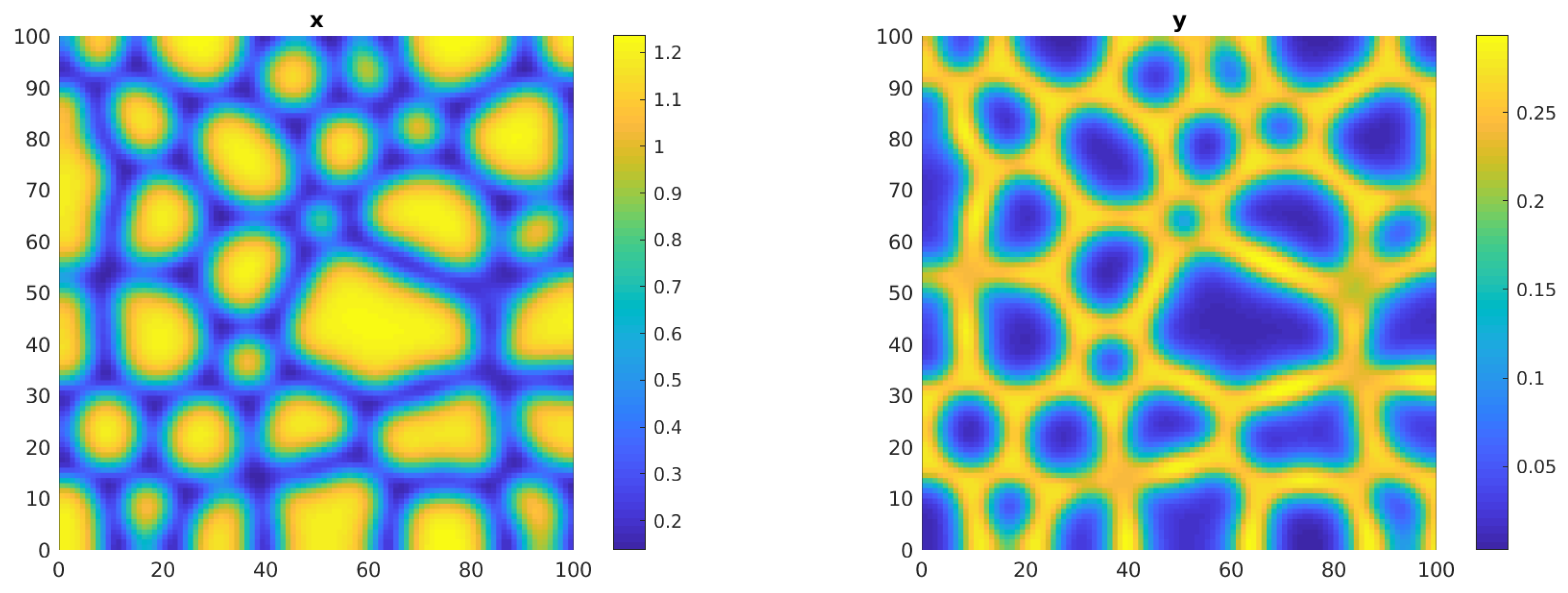
In the first Example we show both the x and y solution, to appreciate the correspondence of patterns in the two functions: due to the choice of positive cross-diffusion coefficients, we always observe that “hot”, or high density zones for one variable correspond to “cold” or low density zones for the other variable at the same location. Because this behavior is common to all the considered examples, in some of the other cases we decided to show the time evolution of just one of the solutions, to illustrate the different patterns without redundancies in the representation.

In all the examples we consider the two dimensional system on the square $[0,100]\times [0,100]$ with no-flux boundary conditions. We always assume as initial condition a small random perturbation of the internal equilibrium $E^{*}$. All the simulations adopt the usual five-point stencil finite difference scheme for the diffusion part, that is treated implicitly, while the nonlinear part is explicitly discretized. The resulting linear system is solved by GMres algorithm. The spatial mesh h is fixed in both directions as 0.5, while the time step is fixed as 0.005. The results have been verified with finer resolution in both space and time without significant differences.

Example 1.

In the parameter settings of Table 2, we first consider the effect of small diffusion rates: we fix ${\gamma }_{11}$ = 0.01, ${\gamma }_{22}$ = 0.1 and ${\gamma }_{12}$ = 0.01. Then it is ${\gamma }_{21}^{cr}$ = 0.01132 and the weakly nonlinear analysis leads to $b_1$, $b_2>$ 0. We set ${\gamma }_{21}$ = 0.015 so that both conditions for the stability of spots and stripes are satisfied and run the simulation on the square [0,100] × [0,100] until the solution stabilizes. Figure 7 shows the mixed spots/stripes pattern predicted by the theoretical analysis on both the x and y solutions. Here, and in all the following figures, high density zones are represented in yellow and low density ones in blue. The simulation time T is reported in the figure caption. In the same parameter setting, with a slight modification of a single diffusion coefficient (${\gamma }_{11}$ = 0.05) the critical value becomes ${\gamma }_{21}^{cr}$ = 0.02437 and again the conditions for the stability of both stripes and spots are met. Once chosen ${\gamma }_{21}$ = 0.032, the following Figure 8 shows how the spots pattern in the x solution evolves eventually into a mixed pattern.

Example 2.

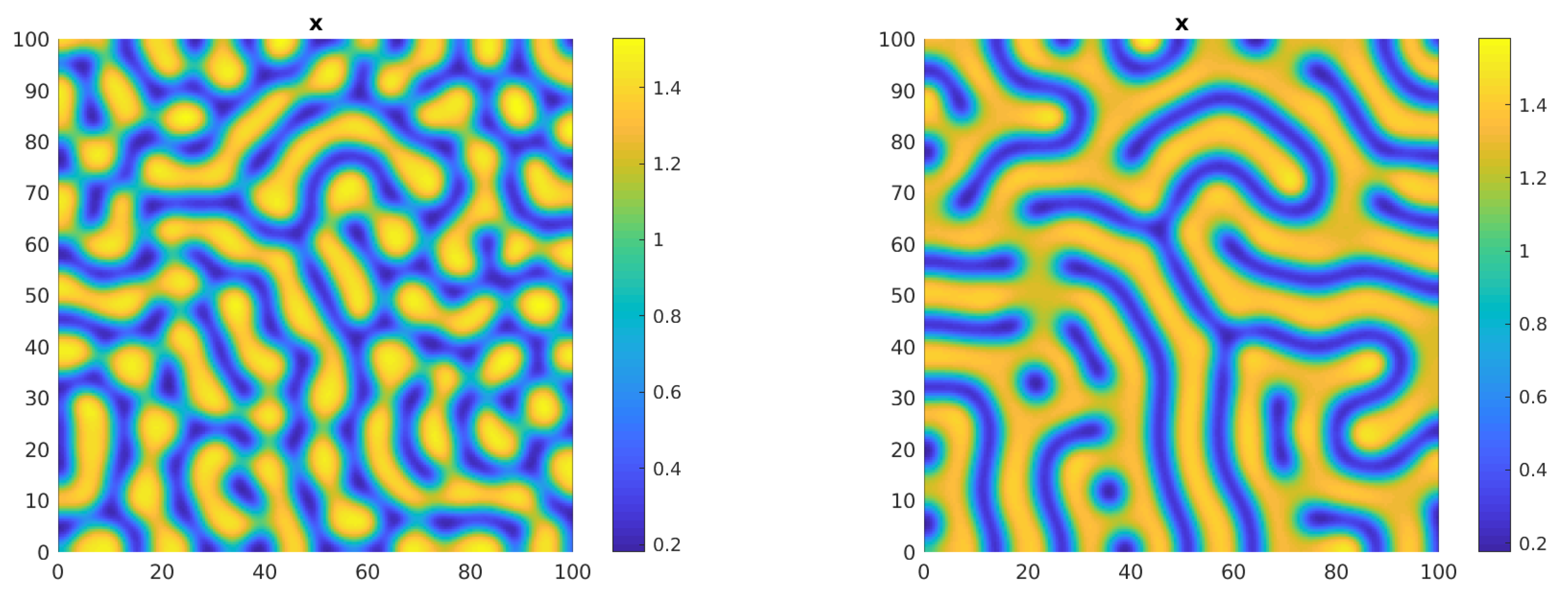
To investigate the effect of higher diffusion rates, we consider ${\gamma }_{11}$ = 1, ${\gamma }_{22}$ = 10 and ${\gamma }_{12}$ = 0.1. Then it is ${\gamma }_{21}^{cr}$ = 1.1628 and the weakly nonlinear analysis leads to $b_1$, $b_2>$ 0. We set ${\gamma }_{21}$ = 1.3 to meet the conditions for the stability of stripes and run the simulations, obtaining patterns that emerge as irregular spots and then stabilizes in the large stripes shown in Figure 9 for time T = 5000. It should be noted how the higher values of the diffusion result in larger patterns.

With a slightly different choice for the diffusion coefficients, ${\gamma }_{11}$ = 0.1, ${\gamma }_{22}$ = 10 and ${\gamma }_{12}$ = 0.01, it is ${\gamma }_{21}^{cr}$ = 0.446 and spots patterns are to be expected from the theory. The following Figure 10, referring to simulations carried out for ${\gamma }_{21}$ = 0.8 up to T = 3000, shows how the pattern stabilizes in large spots, with the usual correspondence between high density zones for one species and low density zones for the other. Let us also show in this parameter setting how different levels of fear $\eta$ affect both the equilibrium value of the predator population and the timing of pattern insurgence: Figure 11 shows simulation results for the predator population in the same setting of Figure 9 when patterns stabilize with different fear levels: in the left panel it is $\eta$ = 0.1 and T = 6000, while in the right panel it is $\eta$ = 1 and T = 4000. These plots should be compared with the bottom right panel of Figure 9. It could be clearly seen that higher fear levels result in lower values for $y^{*}$ and that a similar pattern structure is reached, even if in different simulation times. Moreover, further experiments (not shown here) with even higher values of $\eta$, have proven that excessively enlarging the range of unstable modes can lead to instability of these patterns.

Example 3.

In the two following examples we investigate different parameter settings, leading to different equilibrium points, as detailed in Table 2. By fixing ${\gamma }_{11}$ = 0.25, ${\gamma }_{22}$ = 0.5, ${\gamma }_{12}$ = 0.1, it is ${\gamma }_{21}^{cr}$ = 0.231115 and the weakly nonlinear analysis predicts that stable stripes can occur. We set ${\gamma }_{21}$ = 0.35 and run the simulation. Figure 12 shows the evolution of the x solution from a transient spot pattern (for T = 600) to the expected stable stripes pattern for T = 2000. It should be noted that, due to the chosen diffusions, in this setting the stripes pattern is narrow and differently oriented in different zones of the spatial domain.

Example 4.

In this parameter setting, the internal equilibrium is $E^{*}\approx (0.347,0.209)$; for the spatial system, once fixed ${\gamma }_{11}$ = 0.2, ${\gamma }_{22}$ = 1, ${\gamma }_{12}$ = 0.1, it is ${\gamma }_{21}^{cr}$ = 0.2781 and the weakly nonlinear analysis leads to $b_1$, $b_2>$ 0. We set ${\gamma }_{21}$ = 0.3, very close to the critical threshold so that only the stability conditions for spots are met and run the simulation until the solution stabilizes at about T = 6000. Figure 13 shows the spot patterns predicted by the theoretical analysis for both the x and y solutions.

However, when we choose a higher value for the bifurcation parameter ${\gamma }_{21}$ = 0.35, the spot patterns lose their stability and rapidly evolve into stripes, as the following Figure 14 shows.

5. Conclusions

The spatial distribution of ecological species in their habitat, along with the related governing mechanisms and the consequent scenarios, is a focus of special interest in population dynamics. While self-diffusion terms are used to model the random movement of prey and predator individuals, cross-diffusion terms are included in addition to population models to account for the influence of species interactions on the individuals’ movement. The fundamental mechanisms of these complex spatio-temporal dynamics can be appropriately investigated by means of spatial mathematical models. In this paper we have explored the Turing instability induced by cross-diffusion in a predator–prey system with fear and group defense. In fact, we have found that self-diffusion alone does not induce Turing instability; on the contrary, cross-diffusion is the essential factor causing the occurrence of the spatial patterns. Cross-diffusion-driven instability conditions have been obtained through the linear stability analysis. The cross-diffusion coefficient ${\gamma }_{21}$ has been considered to be the bifurcation parameter and the Turing threshold ${\gamma }_{21}={\gamma }_{21}^{cr}$ has been evaluated numerically and analytically. By performing a weakly nonlinear analysis, we have written the amplitude equations near the Turing bifurcation value and we have obtained the conditions for different shapes of pattern, such as hexagons (spots) and stripes to occur. Numerical simulations have confirmed these theoretical findings in different parameter settings. They have also qualitatively explored the relationship between the high/low value of the diffusion coefficients and the scale of the obtained patterns. Finally, the specific modelling choices resulted in a moderate effect of the fear level on the spatial instability of the internal equilibrium, simply affecting the timing of the insurgence of patterns, in comparison with other models considered in the literature [12,14], where the variation of the fear level induced dramatic changes in the pattern structure. This finding, mainly due to the adopted representation of the group defense, makes the proposed model more suitable to represent different scenarios where, as discussed, fear in prey principally affects predators’ evolution, by lowering their equilibrium value. The methods and findings in this study may provide challenges and ideas on the investigation of spatial pattern formation in other predator–prey systems and in many other fields of applied mathematics. Other aspects of the problem could be examined, such as the Turing–Hopf bifurcations and the consequent oscillating pattern, travelling waves, other response functionals and an eventual comparative study of the effects on the pattern formation scenario.

References

- Cresswell, W. Predation in bird populations. J. Ornithol. 2011, 152, 251–263. [Google Scholar] [CrossRef]
- Preisser, E.; Bolnic, D. The many faces of fear:comparing the pathways and impacts on non consumptive predator effects on prey populations. PLoS ONE 2008, 3, e2465. [Google Scholar] [CrossRef] [PubMed] [Green Version]
- Elliott, K.; Betini, G.; Norris, D. Experimental evidence for within- and cross-seasonal effects of fear on survival and reproduction. J. Anim. Ecol. 2016, 85, 507–515. [Google Scholar] [CrossRef] [PubMed] [Green Version]
- Zanette, L.Y.; White, A.F.; Allen, M.C.; Clinchy, M. Perceived predation risk reduces the number of offspring songbirds produce per year. Science 2011, 334, 1398–1401. [Google Scholar] [CrossRef]
- Hik, D. Does risk of predation influence population dynamics? Evidence from the cyclic declineof snowshoe hares. Wildl. Res. 1995, 22, 115–129. [Google Scholar] [CrossRef]
- Schaller, G.B. The Serengeti Lion: A Study of Predator-Prey Relations; University of Chicago Press: Chicago, IL, USA, 1972. [Google Scholar]
- Tener, J. Muskoxen; Queen’sPrinter: Ottawa, ON, Canada, 1965. [Google Scholar]
- Van Orsdol, K.G. Foraging Behaviour and Hunting Success of Lions in Queen Elizabeth National Park, Uganda. Afr. J. Ecol. 1984, 22, 79–99. [Google Scholar] [CrossRef]
- Ivlev, V. Experimental Ecology of the Feeding of Fishes; Yale University Press: New Haven, CT, USA, 1961. [Google Scholar]
- Sokol, W.; Howell, J.A. Kinetics of phenol oxidation by washed cells. Biotechnol. Bioeng. 1981, 23, 2039–2049. [Google Scholar] [CrossRef]
- Ajraldi, V.; Pittavino, M.; Venturino, E. Modeling herd behavior in population systems. Nonlinear Anal. Real World Appl. 2011, 12, 2319–2338. [Google Scholar] [CrossRef]
- Upadhyay, R.; Mishra, S. Population dynamic consequences of fearful prey in a spatiotemporal predator-prey system. Math. Biosci. Eng. 2018, 16, 338–372. [Google Scholar] [CrossRef]
- Wang, X.; Zanette, L.; Zou, X. Modelling the fear effect in predator–prey interactions. J. Math. Biol. 2016, 73, 1179–1204. [Google Scholar] [CrossRef]
- Mishra, S.; Upadhyay, R.K. Strategies for the existence of spatial patterns in predator–prey communities generated by cross-diffusion. Nonlinear Anal. Real World Appl. 2020, 51, 103018. [Google Scholar] [CrossRef]
- Banerjee, M.; Ghorai, S.; Mukherjee, N. Study of cross-diffusion induced Turing patterns in a ratio-dependent prey-predator model via amplitude equations. Appl. Math. Model. 2018, 55, 383–399. [Google Scholar] [CrossRef]
- Das, M.; Samanta, G.P. A prey-predator fractional order model with fear effect and group defense. Int. J. Dyn. Control 2020. [Google Scholar] [CrossRef]
- Luo, J.; Zhao, Y. Stability and Bifurcation Analysis in a Predator-Prey System with Constant Harvesting and Prey Group Defense. Int. J. Bifurc. Chaos 2017, 27, 1750179. [Google Scholar] [CrossRef]
- Sasmal, S.K.; Takeuchi, Y. Dynamics of a predator-prey system with fear and group defense. J. Math. Anal. Appl. 2020, 481, 123471. [Google Scholar] [CrossRef]
- Rionero, S. Stability of ternary reaction-diffusion dynamical systems. Atti della Accademia Nazionale dei Lincei Classe di Scienze Fisiche Matematiche e Naturali Rendiconti Lincei Matematica E Applicazioni 2011, 22, 245–268. [Google Scholar] [CrossRef]
- Torcicollo, I. On the dynamics of a non-linear Duopoly game model. Int. J. Non-Linear Mech. 2013, 57, 31–38. [Google Scholar] [CrossRef]
- Rionero, S.; Torcicollo, I. Stability of a Continuous Reaction-Diffusion Cournot-Kopel Duopoly Game Model. Acta Appl. Math. 2014, 132, 505–513. [Google Scholar] [CrossRef] [Green Version]
- Rionero, S.; Torcicollo, I. On the dynamics of a nonlinear reaction-diffusion duopoly model. Int. J. Non-Linear Mech. 2018, 99, 105–111. [Google Scholar] [CrossRef]
- Capone, F.; Carfora, M.F.; De Luca, R.; Torcicollo, I. Turing patterns in a reaction-diffusion system modeling hunting cooperation. Math. Comput. Simul. 2019, 165, 172–180. [Google Scholar] [CrossRef]
- De Angelis, F.; De Angelis, M. On solutions to a FitzHugh—Rinzel type model. arXiv 2020, arXiv:1908.00997. [Google Scholar] [CrossRef] [Green Version]
- Murray, J.D. Mathematical Biology I. An Introduction; Interdisciplinary Applied Mathematics; Springer: New York, NY, USA, 2002; Volume 17. [Google Scholar]
- Vanag, V.; Epstein, I. Cross-diffusion and pattern formation in reaction-diffusion systems. Phys. Chem. Chem. Phys. 2009, 11, 897–912. [Google Scholar] [CrossRef] [PubMed]
- Song, D.; Li, C.; Song, Y. Stability and cross-diffusion-driven instability in a diffusive predator–prey system with hunting cooperation functional response. Nonlinear Anal. Real World Appl. 2020, 54, 103106. [Google Scholar] [CrossRef]
- Guin, L.N.; Haque, M.; Mandal, P.K. The spatial patterns through diffusion-driven instability in a predator-prey model. Appl. Math. Model. 2012, 36, 1825–1841. [Google Scholar] [CrossRef]
- Guin, L.N. Existence of spatial patterns in a predator–prey model with self- and cross-diffusion. Appl. Math. Comput. 2014, 226, 320–335. [Google Scholar] [CrossRef]
- Gambino, G.; Lombardo, M.C.; Lupo, S.; Sammartino, M. Super-critical and sub-critical bifurcations in a reaction-diffusion Schnakenberg model with linear cross-diffusion. Ric. Mat. 2016, 65, 449–467. [Google Scholar] [CrossRef] [Green Version]
- Farkas, M. Two ways of modelling cross-diffusion. Nonlinear Anal. Theory Methods Appl. 1997, 30, 1225–1233. [Google Scholar] [CrossRef]
- Shigesada, N.; Kawasaki, K.; Teramoto, E. Spatial segregation of interacting species. J. Theor. Biol. 1979, 79, 83–99. [Google Scholar] [CrossRef]
- Chattopadhyay, J.; Tapaswi, P. Effect of cross-diffusion on pattern formation—A nonlinear analysis. Acta Appl. Math. 1997, 48, 1–12. [Google Scholar] [CrossRef]
- Madzavamuse, A.; Ndakwo, H.S.; Barreira, R. Cross-diffusion-driven instability for reaction-diffusion sydtems:analysis and simulations. J. Math. Biol. 2015, 70, 709–743. [Google Scholar] [CrossRef]
- Torcicollo, I. On the nonlinear stability of a continuous duopoly model with constant conjectural variation. Int. J. Non-Linear Mech. 2016, 81, 268–273. [Google Scholar] [CrossRef] [Green Version]
- Capone, F.; Carfora, M.F.; De Luca, R.; Torcicollo, I. On the dynamics of an intraguild predator–prey model. Math. Comput. Simul. 2018, 149, 17–31. [Google Scholar] [CrossRef]
- Merkin, D. Introduction to the Theory of Stability; Text in Applied Mathematic; Springer: New York, NY, USA, 1997; Volume 24. [Google Scholar]
Figure 1.
Stability regions for the equilibria (blue), (orange), (green) of model (1) in the plane; all the parameter values are chosen as in Table 1.
Figure 2.
Left panel: trajectories of the prey and predator populations from model (1) towards the internal equilibrium E*(0.1734, 0.0273). Right panel: the corresponding phase plane portrait. Parameter values: r = 0.18, = 2.5; all the other values as in Table 1.
Figure 3.
Trajectories of the prey and predator populations from model (1) towards the internal equilibrium E*(0.0591, 0.0113) (left panel) along with the corresponding phase plane portrait (right panel). Parameter values: r = 0.16, = 0.5; all the other values as in Table 1.
Figure 4.
In the left panel, plots of as a function of the wavenumber k for different values of the bifurcation parameter ; in the right panel, a detail of the same plots. Here again , , = 0.01, = 0.1, = 0.01 and other parameter values as in Table 1.
Figure 5.
In the left panel, plots of the real part of the eigenvalue defined in (13) as a function of the wavenumber k for different values of the bifurcation parameter ; in the right panel, a detail of the same plots. Here again , , = 0.01, = 0.1, = 0.01 and other parameter values as in Table 1.
Figure 6.
Plots of as a function of the wavenumber k for different values of the fear level ; in the left panel it is =0.02, in the right panel it is =0.08. Moreover, , , = 0.01, = 0.1, = 0.01 and other parameter values as in Table 1.
Figure 7.
Plots of the solutions of system (2)–(5) in the parameter setting of Example 1 for T = 1500. Here = 0.015. Left panel: x solution, right panel: y solution.
Figure 8.
Plots of the solution x of system (2)–(5) in the parameter setting of Example 1 for T = 1500 (left panel), T = 3000 (right panel). Here = 0.032.
Figure 9.
Plots of the solutions x and y of system (2)–(5) in the parameter setting of Example 2 for T = 2000 (first row) and T = 5000 (second row). Here it is = 1, = 10, = 0.1 and = 1.5.
Figure 10.
Plots of the solutions x and y of system (2)–(5) in the parameter setting of Example 2 for T = 1500 (first row) and T = 3000 (second row). Here = 0.1, = 10, = 0.01 and = 0.8.
Figure 11.
Plots of the solution y of system (2)–(5) in the same parameter setting of Example 2 apart from = 0.1, T = 6000 (left panel) and = 1, T = 4000 (right panel). Here = 1, = 10, = 0.1 and = 1.3. The corresponding equilibrium values for the ODE system (1) are (0.1734, 0.0305) and (0.1374, 0.0243), respectively.
Figure 12.
Plots of the solution x of system (2)–(5) in the parameter setting of Example 3 for T = 500, T = 1000. Here = 0.35.
Figure 13.
Plots of the solutions x (left panel) and y (right panel) of system (2)–(5) in the parameter setting of Example 4 for T = 6000. Here = 0.3.
Figure 14.
Plots of the solution x of system (2)–(5) in the parameter setting of Example 4 for T = 1000 and T = 2000. Patterns for the y solution (not shown) are complementary to these ones. Here = 0.35.