
Study of the Behavior of Cryptocurrencies in Turbulent Times Using Association Rules


1
Unidad Monterrey, Centro de Investigación en Matemáticas, A.C. Av. Alianza Centro 502, PIIT, Apodaca 66628, Mexico
2
Facultad de Ciencias, Universidad Central de Venezuela, Av. Los Ilustres, Esc. de Matemática Piso 3, Los Chaguaramos, Caracas 1020, Venezuela
3
Consejo Nacional de Ciencia y Tecnología, Av. Insurgentes Sur 1582, Col. Crédito Constructor, Ciudad de México 03940, Mexico
*
Author to whom correspondence should be addressed.
Mathematics 2021, 9(14), 1620; https://0-doi-org.brum.beds.ac.uk/10.3390/math9141620
Submission received: 9 June 2021
/
Revised: 24 June 2021
/
Accepted: 6 July 2021
/
Published: 9 July 2021
(This article belongs to the Special Issue Mathematics and Mathematical Physics Applied to Financial Markets)
Abstract
:We studied the effects of the recent financial turbulence of 2020 on the cryptocurrency market, taking into account both prices and volumes from December 2019 to July 2020. Time series were transformed into transaction matrices, and the Apriori algorithm was applied to find the association rules between different currencies, identifying whether the price or the volume of the currencies compose the rules. We divided the data set into two subsets and found that before the decline in cryptocurrency prices, the association rules were generally formed by these prices and that, then, the volumes of the transactions dominated to form the association rules.
1. Introduction
Over the last few years, one topic that has been growing in popularity and has attracted the interest of investors and funds that want to bet on it is cryptocurrencies. A cryptocurrency is nothing more than a digital unit of exchange of value used to send and receive payments through computers that are connected to each other. Also known as cryptocurrencies, these units are essentially software and work through peer-to-peer (P2P) networks on the Internet. In other words, cryptocurrencies comprise a new concept: they are a form of money that works privately between users who possess it and exchange it among themselves. Cryptocurrencies can be bought and exchanged for ”traditional” money and are quoted in markets on which their value is speculated, as is the case with common currencies. Today, more than 22,000 projects are operating within the industry. Such exchanges with low transaction rates and more than 5000 virtual currencies worldwide, combined with a daily trading volume of almost 174 billion dollars, make cryptocurrencies a very attractive investment instrument for the general population [1]. There are different platforms for the exchange of cryptocurrencies, some of the most used of which are CoinBase, Bittrex, Kucoin, among others, which are very effective and secure for users. On their corresponding websites, one can buy, sell, or exchange cryptocurrencies for other digital currencies or trust money (USD, EUR, etc.).
Moreover, association rules are similar to classification rules, and the objective is to find associations or correlations between elements or objects in transactional, relational databases or data warehouses. The classic association pattern mining problem was originally defined in the context of the mining of supermarket data containing sets of items purchased by customers and referred to as transactions. Much of the terminology for this type of problem was borrowed from the “shopping cart analogy”, e.g., the term “transactions” to describe the data sets and the term “item sets” to refer to the results. Generalizing or adopting a use-neutral approach to the application, i.e., an approach that is not related to the “shopping cart analogy”, a frequent pattern can be defined as the universe of all possible sets. The need for the identification of a simple way to understand the problem of association rules in data mining (called the support/confidence network) and the apparent applicability of these kinds of rules for many applications has led to a large number of research papers, the recommendations of which have been used in a wide variety of intelligent business applications to improve decision-making, such as shopping cart analysis [2], customer purchase intention [3], commercial sales analysis [4], custom risk management [5], and time series of stock prices [6]. Association rules have the potential to be very useful for data mining analysts (especially in relation to visualization) and as input for other applications and models. Many of the frequent item set mining and association rule algorithms are based on the Apriori algorithm or modifications of it. In [7,8,9,10], adaptations of the Apriori algorithm as a basic search strategy were presented, but the whole set of procedures and data structures was also adapted. We can highlight that the scheme of this important algorithm has been used not only in basic association rule mining but also in other fields of data mining, such as hierarchical association rules [11,12], association rule maintenance [13,14,15,16], sequential pattern mining [17,18], episode mining [19], and functional dependency discovery [20,21]. However, a practical drawback of mining and the efficient use of association rules is that the set of rules returned by the mining algorithm is often too large to be used directly.
Cryptocurrency trading and investing is more common these days than it was before the 2017 Bitcoin behavior; it represents a new way for many companies to diversify their payment methods and transactions. Furthermore, there are too many professional investors, family funds, and even some hedge funds that have confirmed they are investing in this market or at least in the futures market.
After the financial crisis of 2007–2011, institutions around the world became even more concerned about the development of risk control systems in the banking sector [22,23]. This is because the risk of contagion can have disastrous consequences for the economy. What happened at that time is an example of systemic risk. In finance, systemic risk can be interpreted as potentially catastrophic financial system instability caused by idiosyncratic events or conditions in financial intermediaries [24].
A first work that we conducted following the one discussed above can be read in [25]. In that paper, in the sense of studying systematic risk and contagion between currencies, we used transfer entropy when the cryptocurrency market is in a turbulent situation. Systematic risk is the overall, day-to-day, ongoing risk that can be caused by a combination of factors, such as the economy, interest rates, geopolitical issues, corporate health, and other factors, and also it should not be confused with market risk, which is well known to be present in all markets. In addition, there is literature discussing the spillover effect and systematic risk among cryptocurrency markets. For example [26] shows evidence that Bitcoin tends to be the recipient of the spillover effect, while Ethereum is probably the independent currency in cryptocurrency markets. Huynh et al. [27] found a risk contagion effect between cryptocurrencies when applying a copula approach, so they suggest performing portfolio diversification to avoid this phenomenon.
The contribution of this paper is to apply association rules for discovering the relationships between individuals or a group of currencies by proposing methodological tools based on the Apriori algorithm with the aim of helping detect and characterize systemic risk in cryptocurrency markets. Specifically, schemes are proposed to deal with large volumes of data and draw conclusions through visualization techniques that are indicative when making decisions in crisis scenarios, which can serve as early indications of volatility or turbulence in this market. We can note that there are previous works that use association rules to investigate the behavior of the stock market as well as for cryptocurrencies. Thus, for example, Hajizadeh et al. [28] use some techniques such as decision tree, neural network, association rules, factor analysis, etc. in stock markets. Liao and Chou [29] use association rules and clustering analysis, among other methodologies, to investigate co-movements in Taiwan and China stock markets for future investment portfolios. Han et al. [30] present a market analysis of blockchain-based cryptocurrencies from two perspectives. The first is about the characteristics to be considered in the cryptocurrency market and what can be found when analyzing cryptocurrencies. The second is about detecting abnormal behavior in the cryptocurrency market. Likewise, they show how to detect “pump and dump schemes” in the cryptocurrency market using an improved Apriori algorithm. In Liao et al. [31], they investigate the investment problems in the Taiwan stock market using a data mining approach, wherein a first stage they use association rules and the Apriori algorithm to extract knowledge and illustrate patterns and knowledge rules in order to propose the association of stock categories and possible investment collections in stock categories. Finally, we can mention the work of Ariya [32]; the objective of his study is to apply association rule mining for stock market forecasting. The author selects eight groups of stock to test with this method: financials, agribusiness, consumer products, services, real estate, and construction industry groups, resources, technology, and industry.
Hopefully, these results could be a very useful tool in order to help professionals who venture into investing in these kinds of risky financial instruments to have more quantitative tools to assess systemic risk in times of turbulence.
The remainder of this work is organized as follows. In Section 2, we briefly describe the association rules and the Apriori algorithm. In Section 3, we present a description of the data used and the results obtained from the application of the Apriori algorithm. In Section 4, we present our conclusions and recommendations.
2. Preliminaries
2.1. Association Rules
Association rules are an important class of regularities that exist in databases. They were first introduced in [33], and since then, the problem of associations in mining has received much attention. The classic application of such rules is shopping cart analysis, which analyzes how the items purchased by customers are related. An example of an association rule is as follows:
This rule says that 15% of customers buy cheese and milk together and that those who buy cheese also buy milk 75% of the time. The basic model of the association rules is as follows:
Let be a set of items. Let T be a set of transactions (the database), where each transaction t (a data point) is a set of items such that . An association rule is an implication of the form, , where , and . Rule holds in transaction set T with confidence if % of transactions in T that support X also support Y. The rule has support in T if % of the transactions in T contain . In the example above, the rule has a confidence of 75%, which means that 75% of the transactions in T that support cheese also support milk. The same rule has a support of 15%, i.e., 15% of the transactions in T contain cheese or milk ([33], p. 208).
Association rules are selected from the set of all possible rules using measures of significance and interest. Support, the main measure of significance, is defined as the fraction of transactions in the database that contain all the elements of a specific rule [34]. In other words,
where represents the number of transactions that contain all items in X and Y, and m is the number of transactions in the database [35,36].
The main objective of this algorithm is to determine which operations are performed together, efficiently associate which elements that have similar behaviors, and identify dependency criteria.
There are two properties of association rules that allow us to simplify the structure of the rules. The first property, called the support monotonicity property, tells us that when a set of elements, T, is contained in an operation, all its subsets will also be contained in that operation. Therefore, the support of any subset J of T will always be at least equal to that of T, Formally, we have the following [34]:
Property 1
(Support Monotonicity Property). The support of every subset J of T is at least equal to that of the support of item set T.
Proof.
Suppose the converse, that is, for some and suppose , then J contains elements of database I; but by hypothesis , so every element of J is in T, then is at least s, which contradicts the assumption. □
The monotonicity property of support implies that every subset of a frequent item set will also be frequent. This brings us to the second property, called the downward closure property. This property provides an important constraint on the inherent structure of frequent patterns, which is very convenient from an algorithmic point of view. Frequent pattern extraction algorithms take advantage of this constraint to trim the search process to achieve greater efficiency. In addition, the downward closure property can be used to create concise representations of frequent patterns, in which only the maximum frequent subsets are preserved [34]. A similar idea has been used in theory of siphon in theoretical computer science [37] where the authors define a minimal siphon in a Petri net. Formally, we write this property as follows:
Property 2
(Downward Closure Property). Every subset of a frequent item set is also frequent.
Proof.
Let . Then any set that contains all elements of I also contain all elements of J. Thus, the count of J must be at least as large as the count of I, and if the count of I is at least s, then the count of J is at least s. Since J may be contained in some sets that are missing one or more elements of , then the count of J is strictly larger than the count of I. □
Frequent item sets are used to generate association rules, using a measure known as confidence [34]. The confidence of a rule, , is defined as the conditional probability that an operation contains the set of elements, Y, given that it contains the set of elements, X. This probability is estimated by dividing the support of the element set by that of element set X.
The set of items, X, is referred to as the antecedent, and the set of items, Y, is referred to as the consequence of the rule.
As in the support case, we can use a minimum confidence threshold (minconf) to generate the most relevant association rules. Thus, using both the support and confidence criteria, Aggarwal defined the association rules as follows [34]:
Definition 1
(Association Rules). Let X and Y be two item sets. Then, rule is said to be an association rule at a minimum support of minsup and minimum confidence of minconf if it satisfies the following two criteria:
- The support of item set is at least minsup.
- The confidence of rule is at least minconf.
The first criterion of the above definition ensures that a sufficient number of transactions are relevant to the rule in question; therefore, it has the necessary critical mass to be considered relevant to the application in question. The second criterion ensures that the rule has sufficient strength in terms of conditional probabilities. Thus, both measures quantify different aspects of the association rule.
Given a set of I transactions (the database), the problem with association rules is the need to discover all association rules that have support greater than the minimum support (minsup) and confidence greater than the minimum confidence (minconf), both of which are user-defined quantities. With this in mind, the association rules algorithm is a two-step algorithm:
- Generate all large sets of elements satisfying minsup.
- Generate all association rules satisfying minconf using the large element sets.
The minsup is the key element that makes association rule mining practical and is used to prune the search space to limit the number of rules generated. However, the use of a single minsup implicitly assumes that all items in a database are of the same nature and/or have similar frequencies. However, in real-life applications, this is often not the case. In many applications, some elements appear infrequently in the data, while others appear many times. If the frequencies of the elements in the database vary greatly, then we encounter two problems:
- If the minsup is set too high, then rules involving rare or uncommon items in the data will not be found.
- To find rules involving both frequent and rare items, we have to set minsup to be too low. However, this can cause a combinatorial explosion, producing too many rules because those frequent elements will be associated with each other in every possible way, and many of these associations do not make sense.
A solution to this problem is to discover the frequent item sets, for this the first thing to do is to build a candidate set of item sets and then identify, within this candidate set, those item sets that meet the requirements to be a frequent item set. Generally, this is done iteratively for each frequent k-item set with increasing order of k, where a frequent k-item set is a frequent itemset with k items. There are several algorithms with different characteristics for that purpose, some of them are: AIS [33], SETM [38], Apriori [39], AprioriTID [39], DIC [8], FP-Growth [40], Max-Miner [41], and Eclat [42].
2.2. Apriori Algorithm
In general, it is not difficult to extract rules from the databases; the problem lies in the fact that doing so is very expensive computationally, so much so that it would be impossible to generate them for a database with many products without more detail. Imagine that we have a database with only 10 products, let us name it {A,B,C,D,F,G,H,I,J}. Then, to extract the rules, we must make combinations of these 10 products, so, we have 1024 possible rules (these are the possible combinations between 10 products of various sizes); however, if we have 20 products, then we have 1,048,576 possible combinations. The above situations provide evidence of the problem of using algorithms with exponential complexity.
The following image (Figure 1) shows in detail what is described above for five products: {A,B,C,D,E}.
The Apriori algorithm uses the downward closure property to solve this problem by pruning the candidate search space. This property imposes a clear structure on the set of frequent patterns. In particular, information about the infrequency of the item sets can be used to carefully generate the super set candidates. Therefore, if an item set is infrequent, then the support of its superset candidates is not counted since doing so is meaningless. The following image (Figure 2) shows a visual example of this situation: The first row shows the five items {A,B,C,D,E} and the second row shows all sets of combinations of two items. Suppose that the first set {A,B} is infrequent, then by the downward closing property, all sets of three items in the third row containing A and B will be infrequent. In Figure 2, these are the shaded {A,B,C}, {A,B,D}, and {A,B,E}. The same will be true for four-candidates sets containing A and B; in this case, the sets {A,B,C,D}, {A,B,C,E}, and {A,B,D,C} and finally the set containing {A,B,C,D,E} will also be infrequent. In Figure 2, these infrequent item sets have been framed in the red circle.
The Apriori algorithm starts by generating the shortest k-candidates, in the above example 2-candidates, and counting their supports and then uses the sets of frequent k-elements to generate the length candidates ) (3-candidates of the above example) with the downward closing property. The generation of candidates and the counting of pattern supports with increasing length are interspersed in the Apriori algorithm [34].
Let denote the set of k-frequent elements and denote the set of k-candidate elements. The basis for the approximation consists of iteratively generating -candidates, , from the sets of k-frequent elements in found by the algorithm. For these -candidates, the frequencies are counted with respect to the transaction database. When generating the -candidates, the search space can be reduced by checking whether all k-sets of are included in . If a pair of element sets, X and Y, in have elements in common, then a union between them using the common elements will create a candidate set of element size . Additionally, to avoid redundancy in the generation of the candidates, the convection of imposing a lexicographic order on the items is used. The use of the downward closure property in conjunction with the above convection ensures that there is no redundancy between the candidates, for example, the candidates {A,C,D}, and {A,D,C} constitute the same set so only {A,C,D} appears and also ensure that no truly frequent item sets are lost in the set of candidates. The following two algorithms (Algorithms 1 and 2), show the Apriori algorithm and the function to generate the candidates respectively:
| Algorithm 1 Apriori algorithm |
|
From the above algorithms, we can highlight that the most delicate step is the support computation for all candidates returned by APRIORI-GEN: in particular, the instruction
for a given transaction t. Let be the number of candidates in and the length of t. Assume that is stored in a suitable data structure such as a TRIE (see [43])
- If then generate all subsets of t of size k and add to those that belong to .
- If then scan all candidates in and add to those that are subsets of t.
In any case, the support computation for all candidates can be accomplished in . Consider a data set T of N transactions over a set I of d items and a support threshold minsup. Define as sum of transactions lengths (input size); as sum of lengths of frequent item sets (output size), and as length of the longest frequent item set. The next theorem gives us the complexity of the Apriori algorithm
Theorem 1.
The Apriori algorithm for mining frequent item sets runs in time polynomial in and .
Proof.
Let us determine the contribution of the main steps of the algorithm to the complexity.
- Computation of and : time . Since , the time is .
- APRIORI-GEN(), for :
- ‒
- Candidate generation: time , where denotes the number of frequent item sets of size .
- ‒
- Candidate pruning: time , assuming stored in a TRIE.
- Overall, all executions of APRIORI-GEN require time , hence, time .
- Support counting for , for : time , where denotes the number of candidates of size k. Since , we have that, overall, all support countings require time , hence, time .
□
| Algorithm 2 APRIORI-GEN(F) |
|
3. Results and Discussion
We focused on 131 cryptocurrencies, which were obtained from CoinMarketCap.com (accessed on 8 July 2020) [1], using the CoinMarketCap API, SQL and different Python libraries. Our study covered the period from 1 December 2019 to 5 July 2020, with a sampling frequency of one hour. To apply the Apriori algorithm to the data and see the differences in behavior before and after the stock market crash in March 2020, we worked with three data sets. The first data set (dataset 1) was the complete data file and consisted of 5232 observations, the second data set (dataset 2) spanned from 1 December 2019, at 00:00, to 15 March 2020, at 23:00, and consisted of 2544 observations, and the third data set (dataset 3) spanned from 16 March 2020, at 00:00, to 5 July 2020, at 23:00, and consisted of 2688 observations. We worked with price and volume; thus, to identify in the rules of association whether price or volume is being referred to, we added the suffix “_P” for price and the suffix “_V” for volume to the end of each name. We used the “arules” and “arulesViz” packages in R to study the association rules and the Apriori algorithm [44,45].
To shape this analysis, we had to make some modifications to the database obtained since the association rule algorithms were not designed to study numerical data; however, we created a deterministic function to correctly associate the behavior of cryptocurrencies. The database of the price and volume returns of the 131 cryptocurrencies was transformed into a matrix of “zeros” and “ones” through an indicator function, given in the following way:
The intention of changing our numerical data to factors of the type “zeros and ones” was to be able to identify when the value of a cryptocurrency went up or down. Recall that the Apriori algorithm works with items, so it creates a rule if the item is present, but in our case all the rows of the database contain all the items, that is, the daily closing prices. Therefore, to solve this fact and have a transaction database similar to what is used for the Apriori algorithm, we create an indicator-matrix through the function given by (3). For example, if the price of Bitcoin went up, then the return would be positive, and we would place a 1 in the auxiliary matrix. Conversely, if the price went down, then the return would be negative, and we would place a 0 in the auxiliary matrix. We did the same with all the cryptocurrencies so that the Apriori algorithm could establish the association rules between them. For example, suppose that Bitcoin and Ethereum prices go up on d day and that same day Binance USD price goes down, then in the auxiliary matrix, for Bitcoin and Ethereum will appear a 1 and for Binance USD will appear a 0, so that the Apriori algorithm will create a rule with Bitcoin and Ethereum but not with Binance USD. Huang et al. use a similar procedure in [6] to prepare the data and transform it into a transaction database.
We work with the log returns of price and volume for each cryptocurrency. In Table 1, we show a summary of the mean values of some statistics for the association rules: support, confidence, lift, count, coverage, and the chi-squared statistic to test for independence between the LHS and RHS (The left-hand side (LHS) is the antecedent, and the right-hand side (RHS) is the consequence of the rule) of the rule [36]. The complete subsets are Set1, Set2 and Set3; the subsets without redundant rules are Set1a, Set2a and Set3a (Rule is redundant if ); and the subsets with support greater than and confidence greater than are Subset1, Subset2 and Subset3. For the latter three sets, the subsets obtained are “Subset 1”, with support greater than the 99th quantile and confidence greater than the 95th quantile, obtaining 100 rules; “Subset 2”, with support greater than the 99th quantile and confidence greater than the 90th quantile, reducing to 116 rules; and “Subset 3”, with support and confidence greater than the 99th quantile, reducing the number of rules from 14,512,698 to 495. There are several algorithms for finding the “best”, “optimal”, or “most interesting” rule(s) in a database. These different algorithms use a variety of metrics such as confidence, support, gain, Chi-square value, Gini, entropy gain, Laplace, lift, and conviction. Bayardo and Agrawal [46] show that the best rule according to any of the above metrics should reside on a support/confidence frontier, so for that reason, the rules with the highest support and confidence were taken for this study.
In Table 2, the first 10 rules of Subset 1 are shown for dataset 1, ordered by confidence. We can see, for example, that the first rule tells us that positive volume returns on Bitcoin, Ethereum, EOS, and Binance USD lead to a positive volume return on Tether with 97.3% confidence and that the positive volume return on these 5 cryptocurrencies together occurs in 25.6% of the transactions. The chi-square statistic for this rule is 1794.4, which indicates that the LHS and RHS are not independent.
In Subset 1, as seen in Table 1, 100 association rules are formed by 30 different cryptocurrencies as antecedents (LHS) and four cryptocurrencies as consequences (RHS). Among the cryptocurrencies on the LHS, we can highlight “Ethereum” (price) forming 56 of the 100 rules, “Bitcoin Cash” (price) forming 51 rules and “EOS” (price) forming 31 rules. The currencies on the RHS are “Bitcoin” (price), with 80 rules; “Ethereum” (price), with 14 rules; “Tether” (volume), with 4 rules; and “Binance USD” (price), with 2 rules. In Figure 3, part (a), we can observe the 100 association rules of Subset 1 grouped into 10 groups (Figure 3, Figure 4, Figure 5, Figure 6, Figure 7 and Figure 8 were made with R package arulesViz [47].) On the x-axis, the size of the circle denotes the support, and the color denotes the same lift in each group. From left to right, we can see a first group with four rules and, as a consequence, the volume return of “Tether” with a mean support of 0.266 and lift greater than 1.983. In the second group, 2 rules appear with the consequence of price return of “Binance USD”; the rules that conform to this group are rules 1 and 3, which have a mean support of 0.314 and 0.287 and lift of 1.911 and 1.935, respectively. Groups 4 and 6 have as a consequence (RHS) the price return of “Ethereum” with a mean support 0.254 and lift of 1.862. In these two groups, there are 14 rules, and finally, the remaining 80 rules are grouped into groups 3, 5, 7, 8, 8, 9, and 10 with a consequence of price return of “Bitcoin”. In part (b) of Figure 3, we can observe a support and confidence dispersion matrix for these 100 rules, where the color indicates the order of the rules (LHS + RHS) (The order of an association rule is the number of items (coins) that form it on the LHS and RHS. In our case, on the RHS, there is only one item for all the rules and different numbers of items on the LHS). For order 4 (LHS = 3 + RHS = 1), we have two rules with confidence values between 0.9580 and 0.9587 and support values between 0.297 and 0.314. For order 5 (LHS = 4 + RHS = 1), we have 53 rules with confidence values between 0.957 and 0.973 and support values between 0.250 and 0.286. For order 6 (LHS = 5 + RHS = 1), we have 45 rules with confidence values between 0.956 and 0.966 and support values between 0.250 and 0.262.
In Figure 4, we can see a matrix with the association rules for Subset 1, in which we can observe on the x-axis from left to right, the antecedents (LHS), and on the y-axis, the consequences (RHS). From the bottom, the first value corresponds to the rules with the consequence of the price return of “Binance USD”. In this case, rules 1 and 3 have as a consequence that currency has confidence values of 0.958 and 0.970 for each rule and lift of 1.910 and 1.934, respectively. The second value corresponds to the rules with the consequence of the price return of “Bitcoin”; these 80 rules have confidence values between 0.957 and 0.970 and lift between 1.848 and 1.874. The third value corresponds to the 14 rules that have the consequence of the price return of “Ethereum”, with confidence values between 0.956 and 0.962 and lift values between 1.858 and 1.869. Finally, the last value corresponds to the rules with a consequence of the volume return of “Tether”, with confidence values between 0.958 and 0.973 and lift between 1.983 and 2.012.
Subset 2, as we indicated above, spanned from 1 December 2019, to 15 March 2020, with 2544 association rules. In this subset, as seen in Table 1, we obtained 116 association rules formed by 29 cryptocurrencies as antecedents (LHS) and five cryptocurrencies as consequences (RHS). Among the cryptocurrencies on the LHS, we can highlight “EOS” (price return) forming 45 of the 116 rules, “Bitcoin” (price return) forming 43 of the rules, and “Bitcoin Cash” (price return) forming 37 of the rules. The cryptocurrencies on the RHS are “Ethereum” (price return) in 57 rules, “Bitcoin” price return in 40 rules and volume return in five rules, “Tether” (volume return) in 11 rules, and “Binance USD” (price return) in 3 rules.
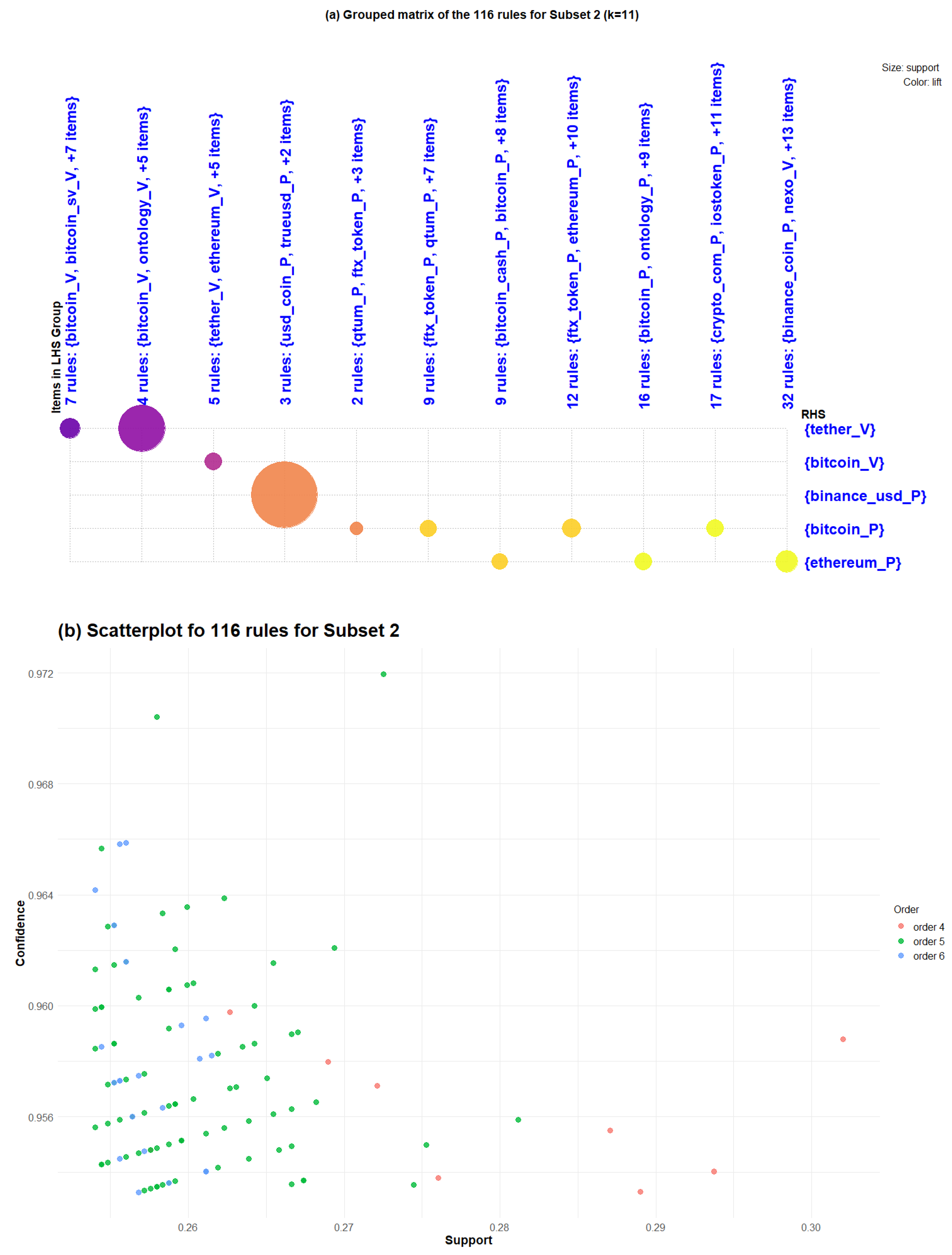
In Figure 5, part (a), we can observe the 116 association rules of Subset 2 grouped into 11 groups. From left to right, we can see a first group with seven rules that have a consequence of the “Tether” volume return with medium and high lift support. In the second group, there are another four rules with consequences: the volume return of “Tether” with high support and high lift. Group 3 has five rules, the consequence of which is the volume return of “Bitcoin” with medium support (0.2586) and medium lift (1.928). Group 4 has a consequence of the price return of “Binance USD” and consists of three rules, with a support of 0.2894 and lift of 1.900. Groups 5, 7, and 9 have a consequence (RHS) of the return of “Bitcoin” prices with low support and low lift; in these three groups, there are 40 rules. Finally, groups 6, 8, 10, and 11 contain the remaining 57 rules with a consequence of the return of “Ethereum” prices, with low support and low lift. In part (b) of the same Figure 5, we can observe a support and confidence dispersion matrix for these 116 rules, where the color indicates the order of the rules (LHS + RHS). For this case, we have rules of orders 4, 5, and 6. The 11 rules of order 4 (LHS = 3 + RHS = 1) have confidence values between 0.953 and 0.960 and support values between 0.256 and 0.302. The 83 rules of order 5 (LHS = 4 + RHS = 1) have confidence values between 0.953 and 0.972 and support values between 0.254; 0.281. The 22 rules of order 6 (LHS = 5 + RHS = 1) have confidence values between 0.953 and 0.966 and support values between 0.254 and 0.262.
In Figure 6, we can see a matrix with the association rules for Subset 2; on the x-axis, the antecedents (LHS) are shown, and on the y-axis, the consequences (RHS) are shown. The first value corresponds to the three rules a consequence of the price return of “Binance USD”, with lift between 1.855 and 1.920 and confidence between 0.954 and 0.971. The second value corresponds to the 40 rules that have a consequence of the price return of “Bitcoin”, with lift between 1.864 and 1.898 and confidence between 0.953 and 0.970. The third value, , corresponds to the five rules that have a consequence of the volume return of “Bitcoin”, with lift between 1.919 and 1.935 and confidence between 0.955 and 0.962. The fourth value corresponds to the rules with a consequence of the price return of “Ethereum”. These 57 rules have lift between 1.859 and 1.883 and confidence between 0.953 and 0.965. Finally, the fifth value corresponds to the 11 rules with a consequence of the volume return of “Tether”, with lift between 1.933 and 1.954 and confidence between 0.953 and 0.963.
Subset 3 starts on 16 March 2020 and ends on 5 July 2020, with 2688 association rules. In the case of Table 1, the “Subset 3” consists of 495 association rules formed by 31 cryptocurrencies as antecedents (LHS) and four cryptocurrencies as consequences (RHS). Among the cryptocurrencies on the LHS, we can highlight that the price return of “Bitcoin” forms 460 rules, the price return of “Binance USD” forms 333 rules, the price return of “Bitcoin Cash” forms 174 rules, and the price return of “Ethereum” forms 171 rules. The cryptocurrencies considered consequential (RHS) are “FTX Token” (price return), forming 473 of the 495 rules; “Bitcoin” (price return), forming 19 rules; “Tether” (volume return), forming 2 rules; and “Binance USD” (price return), forming 1 rule.
In Figure 7, part (a), we can observe the 495 association rules of Subset 3 grouped into 20 groups. From left to right, we can see a first group with two rules that have a consequence of the volume return of `Tether’, with a mean support of 0.252 and lift of 2.064. The second group has only one rule with a consequence of the price return of “Binance USD”, with a mean support of 0.251 and lift of 1.966. Groups 3 to 19 have a consequence (RHS) of the price return of “FTX Token”, with support between 0.249 and 0.311 and lift between 1.864 and 1.886; in these 17 groups, there are 473 rules. Finally, group 20 contains the remaining 19 rules with a consequence of the price return of “Bitcoin”, with a mean support of 0.255 and a mean lift of 1.858. In part (b) of the same Figure 7, we can observe the support and confidence dispersion matrix for these 495 rules. For this case, we have rules of orders 5, 6, and 7. The 111 rules of order 5 (LHS = 4 + RHS = 1) have confidence values between 0.971 and 0.983 and support values between 0.249 and 0.312. The 346 rules of order 6 (LHS = 5 + RHS = 1) have confidence values between 0.971 and 0.982 and support values between 0.249 and 0.284. The 38 rules of order 7 (LHS = 6 + RHS = 1) have confidence values between 0.972 and 0.982 and support values between 0.249 and 0.262.
In Figure 8, we can see a matrix with the association rules for Subset 3. The x-axis shows the antecedents (LHS), and the y-axis shows the consequences (RHS). From the bottom, we have the price return of “Binance USD”, as a consequence of one rule, with a confidence value of 0.976 and a lift value of 1.966. Second, we have 19 rules corresponding to the rules with a consequence of the price return of “Bitcoin”. These rules have confidence values between 0.971 and 0.976 and lift values between 1.854 and 1.864. Third, we have 473 rules with a consequence of the price return of “FTX Token”, with confidence values between 0.971 and 0.982 and lift values between 1.864 and 1.886. Looking at Figure 4, we can see that there is a change in RHS for the association rules, for the full period one of the currencies in RHS is the Ethereum price return, while for the period after 11 March 2020, it changes to the FTX Token price return. The same is observed when comparing Figure 6 and Figure 8. Finally, there are two rules with a consequence of the volume return of “Tether”; the rules that have this consequence are rules 1 and 2, with confidence values of 0.983 and 0.977 and lift values of 2.071 and 2.059, respectively.
We can see that behavior differs in Subsets 2 and 3 before and after the beginning of the COVID-19 outbreak on March 11, 2020, the day the World Health Organization (WHO) characterized and declared COVID-19 as a pandemic [48].
In Figure 9, we can observe a directed graph of the 100 association rules of “Subset 1”. We can observe the main network with 94 rules. We can also see, in the center, the price returns of “Ethereum” and “Bitcoin”. These currencies are the main consequences (RHS) of the association rules, appearing in those 94 rules. Similarly, we can observe two separate groups with few rules that are not part of the network, for example, we have a group with rules 1 and 3 that is not connected to the main network. The other group (sub network) that is not connected with the main network is that formed by rules 2, 4, 5, and 6, the items (LHS and RHS) of which are the volume returns of “EOS”, “Tether”, “Ethereum”, “Bitcoin”, “Litecoin”, and “Bitcoin Cash”. From the above findings, we can deduce that the behavior of the crypto-asset market during the period studied was, in general, influenced by the price of the strongest cryptocurrencies. In Figure 10, the flow or direction from the antecedents (LHS) to the consequences (RHS) for the 100 association rules of “Subset 1” shown in Figure 9 can be visualized. On the far left side are 28 coins out of the 30 that make up the antecedents of the association rules. In the center of the Sankey diagram, we can observe the Ethereum price return, which is an antecedent of 56 of the rules and a consequence of another 14 rules. On the far right side, we can see, at the top, the price return of Bitcoin, which appears as an antecedent in 14 rules and as a consequence in 80 rules. Additionally, we can observe Tether (return volume) and Binance USD (return price), which are the two remaining currencies that make up the consequences of these 100 association rules.
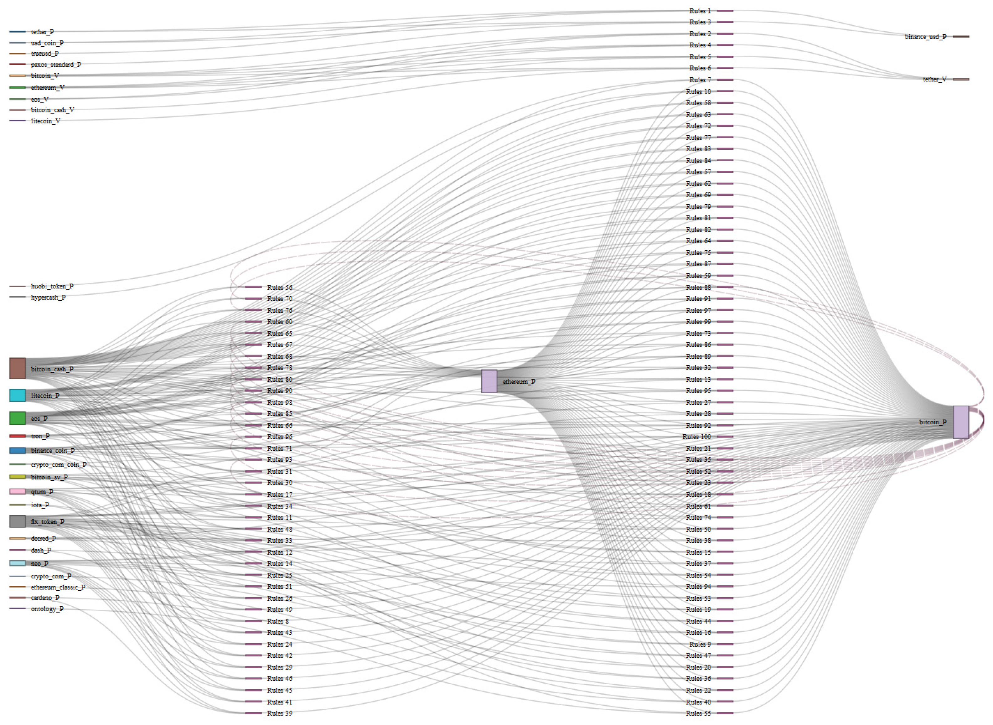
Figure 11 shows the graph of the 116 rules of “Subset 2”. We can see a main network formed by 97 rules with the price returns of “Ethereum”, “Bitcoin”, and “EOS” in the center of the graph. The first two cryptocurrencies account for 97 of the rules as a consequence (RHS), and the third one appears as an antecedent for 45 rules. As in the previous case, we can observe two subnetworks that are not part of the main network, formed by 19 rules between both subnetworks. Among these, we see the volume returns of 10 different coins on both the LHS and RHS, so we can conclude that in this period before the beginning of the pandemic dominated the market, the prices of these cryptocurrencies were in the top 10 of all cryptocurrencies. In Figure 12, as in Figure 10, we can visualize the flow of the 116 association rules for “Subset 2”. The 25 coins on the far left side only form the antecedents (LHS) of the rules, while the coins in the center and on the far right side form both the antecedents (LHS) and the consequences (RHS) of different association rules.
In Figure 13, we can observe in (a) the directed graph of the 495 rules of “Subset 3”, which shows the network formed by 492 rules. In the center (b), we can observe the price returns of “FTX Token” and “Bitcoin” as a consequence of the 492 rules. We can also observe three rules that are not part of the network. In (c), we can see a sub network with two rules, the items of which are the volume returns of “EOS”, “Bitcoin”, “Ethereum”, “Binance USD”, “Bitcoin Cash”, and “Tether”. In (d), we can see a sub network with one rule, the items of which are the price returns of “Tether”, “USD Coin”, “Unus Sed Leo”, and “Binance USD”. We can discard both sub networks because they are not part of the main network. In this case, we see a change in market behavior after 15 March 2020, the main currency of which is “FTX Token”.
In Figure 14, we can observe the behavior of the main currency as a consequence for each subset studied. In (a), the price return of Bitcoin (“Subset 1”) is shown, where we observe the sharp price drop around 15 March 2020, when COVID-19 was declared a pandemic; the same is observed in (b) for Ethereum price returns (“Subset 2”). In contrast, in (c), we can observe the behavior of the price returns of FTX Token (“Subset 3”). We observe a large variation (peak) in mid-February 2020, but around 15 March 2020, the variation in price returns is not as marked as in the other two cases.
4. Conclusions
From the results and analysis in the previous section, we can conclude that the overall behavior of the partnership rules from December 2019 to July 2020 was dominated by cryptocurrency prices, as reflected in all subsets. For example, in “Subset 1”, 96% was formed by price returns and 4% by volume returns. In “Subset 2”, covering the period from December 2019 to 15 March 2020, 84.48% of the best rules (in terms of confidence) was formed by cryptocurrency price, 13.79% by volume, and 1.72% by the combination of price and volume. Conversely, from 16 March 2020, to July 2020 (“Subset 3”), the association rules were almost entirely (99.59%) composed only of price returns and a mere 0.41% of volume returns.
As we have found in this study, the cryptocurrencies with the highest market capitalization in terms of price and volume are those that actually can determine the main market movements, as well as the rules that we have found both in support and in confidence. For example, as we saw in the previous section, there was a change in market behavior after 15 March 2020, whose main cryptocurrency changed from “Bitcoin” and “Ethereum” to “FTX Token”, which may be one of the reasons why investors bet on this cryptocurrency after the turbulence in the economy due to COVID-19. On the other hand, the cryptocurrencies with the highest market capitalization in terms of price and volume may play the role of market benchmark, having good support in the identified rules. In this way, we can conclude that in times of great market volatility, as we experienced last year with COVID-19, with the crashing of the airline, hotel, and cruise industries, these kinds of assets have emerged as an alternative to safeguard capital. This is similar to the case of gold, which has been used as a form of safe haven or store of value since the beginning of the economy, with such use peaking during times of crisis, as has happened to many cryptocurrencies in recent months. One of the best known strategies to mitigate market risk is the diversification of capital, and because many brokers and brokerage houses worldwide have adopted the option of offering contracts for difference (CFDs) for these cryptocurrencies on their platforms, they have been a good option in these last very difficult months for the market. This last point was not experienced in the global financial crisis of 2008 since Bitcoin, in particular, was created in 2009.
As future work, it is proposed to work with time windows in the time series of cryptocurrency records in order to try to get the possible anomalies or risks more efficiently, and it is also proposed to combine digital assets with classical assets so that they can be found if there is an association between these assets and how they affect the stock market one to another, especially with what has to do with systemic risks. Other works propose using the FP-Growth and Eclat algorithms to find the frequent items; these algorithms improve performance and are more computationally efficient. However, its current implementation only allows working with relatively small databases so it remains an open problem to developed for large databases. Another problem that can be addressed is to use a variant of the Apriori algorithm, making use of some measure of interest to prune candidate sets in databases containing numerical attributes.
Author Contributions
Conceptualization: J.B.H.C., A.G.-M. and M.A.P.V.; methodology: J.B.H.C., A.G.-M. and M.A.P.V.; formal analysis: J.B.H.C. and A.G.-M.; investigation: J.B.H.C. and A.G.-M.; resources: A.G.-M.; data curation: J.B.H.C. and A.G.-M.; writing—original draft preparation: J.B.H.C. and A.G.-M.; writing—review and editing: J.B.H.C., A.G.-M., and M.A.P.V.; project administration: A.G.-M.; funding acquisition: A.G.-M. All authors have read and agreed to the published version of the manuscript.
Funding
This research was funded by the government of Mexico through CONACYT, FOSEC SEP-INVESTIGACION BASICA, grant number A1-S-43514.
Institutional Review Board Statement
Not applicable.
Informed Consent Statement
Not applicable.
Data Availability Statement
Not applicable.
Acknowledgments
We wish to thank the anonymous reviewers who undoubtedly helped to enrich different aspects of this work.
Conflicts of Interest
The authors declare no conflict of interest. The funders had no role in the design of the study; in the collection, analyses, or interpretation of data; in the writing of the manuscript; or in the decision to publish the results.
References
- CoinMarketCap. Available online: https://coinmarketcap.com/ (accessed on 8 July 2020).
- Regina Langer, A.O.; Conrad, S. TARtool: A Temporal Dataset Generator for Market Basket Analysis. In Proceedings of the 4th International Conference on Advance Data Minig and Applications (ADMA), Chengdu, China, 8–10 October 2008; pp. 400–410. [Google Scholar]
- Kim, J.W.; Han, S.Y.; Kim, D.S. Association rules application to identify customer purchase intention in a real-time marketing communication tool. In Proceedings of the Fourth International Conference on Ubiquitous and Future Networks (ICUFN), Phuket, Thailand, 4–6 July 2012; pp. 88–90. [Google Scholar]
- Han, B.; Li, Y. Research and Application of Association Rules Methods in Data Mining for Commercial Sales Analysis. In Proceedings of the International Conference on Networking and Digital Society, Guiyang, China, 30–11 May 2009; pp. 183–185. [Google Scholar]
- Wang, Y.; Song, Y. Classification Model Based on Association Rules in Customs Risk Management Application. In Proceedings of the International Conference on Intelligent System Design and Engineering Application, Changsha, China, 13–14 October 2010; pp. 436–439. [Google Scholar]
- Huang, C.; Chen, Y.; Chen, A. An Association Mining Methods for Time Series and Its Application in the Stock Price of TFT-LCD. In Proceedings of the 4th Industrial Conference on Data Minig (ICDM), Leipzig, Germany, 4–7 July 2004; pp. 117–126. [Google Scholar]
- Park, J.S.; Chen, M.S.; Yu, P.S. An Effective Hash-Based Algorithm for Mining Association Rules. ACM Sigmod Rec. 1995, 24, 175–186. [Google Scholar] [CrossRef]
- Brin, S.; Motwani, R.; Ullmam, J.D.; Tsur, S. Dynamic itemset counting and implication rules for market basket data. In Proceedings of the ACM SIGMOD International Conference on Management of Data, Tucson, AZ, USA, 11–15 May 1997; pp. 255–264. [Google Scholar]
- Savasere, A.; Omiecinski, E.; Navathe, S.B. An Efficient Algorithm for Mining Association Rules in Large Databases. In Proceedings of the 21th International Conference on Very Large Data Bases, Zurich, Switzerland, 11–15 September 1995; pp. 432–444. [Google Scholar]
- Toivonen, H. Sampling Large Databases for Association Rules. In Proceedings of the 22th International Conference on Very Large Data Bases, Mumbai, India, 3–6 September 1996; pp. 134–145. [Google Scholar]
- Srikant, R.; Agrawal, R. Mining Generalized Association Rules. In Proceedings of the 21th International Conference on Very Large Data Bases, Zurich, Switzerland, 11–15 September 1995; pp. 407–419. [Google Scholar]
- Han, J.; Fu, Y. Discovery of Multiple-Level Association Rules from Large Databases. In Proceedings of the 21th International Conference on Very Large Data Bases, Zurich, Switzerland, 11–15 September 1995; pp. 420–431. [Google Scholar]
- Cheung, D.W.; Han, J.; Ng, V.T.; Wong, C.Y. Maintenance of discovered association rules in large databases: An incremental updating technique. In Proceedings of the Twelfth International Conference on Data Engineering, New Orleans, LA, USA, 26 February–1 March 1996; pp. 106–114. [Google Scholar]
- Cheung, D.W.; Lee, S.D.; Kao, B. A General Incremental Technique for Maintaining Discovered Association Rules. In Proceedings of the Fifth International Conference on Database Systems for Advanced Applications (DASFAA), Melbourne, Australia, 1–4 April 1997; pp. 185–194. [Google Scholar]
- Thomas, S.; Bodagala, S.; Alsabti, K.; Ranka, S. An Efficient Algorithm for the Incremental Updation of Association Rules in Large Databases. In Proceedings of the Third International Conference on Knowledge Discovery and Data Mining (KDD-97), Newport Beach, CA, USA, 14–17 August 1997; pp. 263–266. [Google Scholar]
- Ayan, N.F.; Tansel, A.U.; Arkun, E. An Efficient Algorithm to Update Large Itemsets with Early Pruning. In Proceedings of the Fifth ACM SIGKDD International Conference on Knowledge Discovery and Data Mining, San Diego, CA, USA, 15–18 August 1999; pp. 287–291. [Google Scholar]
- Agrawal, R.; Srikant, R. Mining sequential patterns. In Proceedings of the Eleventh International Conference on Data Engineering, Taipei, Taiwan, 6–10 March 1995; pp. 3–14. [Google Scholar]
- Srikant, R.; Agrawal, R. Mining Sequential Patterns: Generalizations and Performance Improvements. In Proceedings of the 5th International Conference on Extending Database Technology: Advances in Database Technology, Avignon, France, 25–29 March 1996; pp. 3–17. [Google Scholar]
- Mannila, H.; Toivonen, H.; Verkamo, A.I. Discovering Frequent Episodes in Sequences Extended Abstract. In Proceedings of the First International Conference on Knowledge Discovery and Data Mining, Montreal, QC, Canada, 20–21 August 1995; pp. 210–215. [Google Scholar]
- Huhtala, Y.; Kärkkäinen, J.; Porkka, P.; Toivonen, H. Tane: An Efficient Algorithm for Discovering Functional and Approximate Dependencies. Comput. J. 1999, 42, 100–111. [Google Scholar] [CrossRef] [Green Version]
- Huhtala, Y.; Kärkkäinen, J.; Porkka, P.; Toivonen, H. Efficient discovery of functional and approximate dependencies using partitions. In Proceedings of the 14th International Conference on Data Engineering, Orlando, FL, USA, 23–27 February 1998; pp. 392–401. [Google Scholar]
- Board of Governors of the Federal Reserve System. Lessons from the Failure of Lehman Brothers. Available online: https://www.federalreserve.gov/newsevents/testimony/bernanke20100420a.htm (accessed on 23 June 2021).
- Federal Reserve History. The Great Recession. Available online: https://www.federalreservehistory.org/essays/great-recession-of-200709 (accessed on 23 June 2021).
- Schwarcz, S.L. Systemic Risk. Duke Law School Legal Studies Paper No. 163. Georget. Law J. 2008, 97. Available online: https://ssrn.com/abstract=1008326 (accessed on 23 June 2021).
- García-Medina, A.; Hernández C, J.B. Network Analysis of Multivariate Transfer Entropy of Cryptocurrencies in Times of Turbulence. Entropy 2020, 22, 760. [Google Scholar] [CrossRef]
- Huynh, T.L.D. Spillover risks on cryptocurrency markets: A look from VAR-SVAR granger causality and student’st copulas. J. Risk Financ. Manag. 2019, 12, 52. [Google Scholar] [CrossRef] [Green Version]
- Huynh, T.L.D.; Nguyen, S.P.; Duong, D. Contagion risk measured by return among cryptocurrencies. In International Econometric Conference of Vietnam; Springer: Berlin/Heidelberg, Germany, 2018; pp. 987–998. [Google Scholar]
- Hajizadeh, E.; Ardakani, H.D.; Shahrabi, J. Application of data mining techniques in stock markets: A survey. J. Econ. Int. Financ. 2010, 2, 109–118. [Google Scholar]
- Liao, S.-H.; Chou, S.-Y. Data mining investigation of co-movements on the Taiwan and China stock markets for future investment portfolio. Expert Syst. Appl. 2013, 40, 1542–1554. [Google Scholar] [CrossRef]
- Han, Q.; Wu, J.; Chen, W.; Xu, Y.; Zheng, Z. Chapter 6: Market Analysis of Blockchain-Based Cryptocurrencies. In Blockchain Intelligence Methods, Applications and Challenges; Springer: Singapore, 2021; pp. 135–158. [Google Scholar]
- Liao, S.-H.; Ho, H.-H.; Lin, H.-W. Mining stock category association and cluster on Taiwan stock market. Expert Syst. Appl. 2008, 35, 19–29. [Google Scholar] [CrossRef]
- Ariya, A. Stock Forecasting by Association Rule Mining. In Proceedings of the 21st Asia-Pacific Conference on Global Business, Economics, Finance & Social Sciences (AP18Taiwan Conference), Taipei, Taiwan, 21–22 December 2018. [Google Scholar]
- Agrawal, R.; Imielinski, T.; Swami, A. Mining Association Rules between Sets of Items in Large Databases. In Proceedings of the ACM SIGMOD International Conference on Management of Data, Washington, DC, USA, 25–28 May 1993; pp. 207–216. [Google Scholar]
- Aggarwal, C.C. Data Mining: The Textbook, 1st ed.; Springer: New York, NY, USA, 2015. [Google Scholar]
- Hahsler, M.; Hornik, K. New Probabilistic Interest Measures for Association Rules. Intell. Data Anal. 2007, 11, 437–455. [Google Scholar] [CrossRef] [Green Version]
- Liu, B.; Hsu, W.; Ma, Y. Mining Association Rules with Multiple Minimum Support. In Proceedings of the ACM SIGKDD International Conference on Knowledge Discovery & Data Mining, San Diego, CA, USA, 15–18 August 1999; pp. 337–341. [Google Scholar]
- Shang, Y. Consensus formation in networks with neighbor-dependent synergy and observer effect. Commun. Nonlinear Sci. Numer. Simul. 2021, 95, 105632. [Google Scholar] [CrossRef]
- Houtsma, M.; Swami, A. Set-Oriented Mining for Association Rules; IBM Research Report RJ9567; IBM Almaden Research Center: San Jose, CA, USA, October 1993. [Google Scholar]
- Agrawal, R.; Srikant, R. Fast Algorithms for Mining Association Rules. In Proceedings of the 20th International Conference on Very Large Data Bases (VLDB’94), Santiago de Chile, Chile, 12–15 September 1994; pp. 487–499. [Google Scholar]
- Han, J.; Pei, J.; Yin, Y. Mining Frequent Patterns without Candidate Generation. In Proceedings of the 2000 ACM SIGMOD International Conference on Management of Data, Dallas, TX, USA, 15–18 May 2000; pp. 1–12. [Google Scholar]
- Bayardo, R.J., Jr. Efficiently mining long patterns from databases. In Proceedings of the ACM SIGMOD International Conference on Management of Data, Seattle, WA, USA, 2–4 June 1998; pp. 85–93. [Google Scholar]
- Zaki, M.J.; Parthasarathy, S.; Ogihara, M.; Li, W. New algorithms for fast discovery of association rules. In Proceedings of the Third International Conference on Knowledge Discovery and Data Mining (KDD’97), New Port Beach, CA, USA, 14–17 August 1997; pp. 283–286. [Google Scholar]
- Sedgewick, R.; Wayne, K. Algorithms, 4th ed.; Addison-Wesley Professional: Reading, MA, USA, 2011; Chapter 5. [Google Scholar]
- Hahsler, M.; Buchta, C.; Gruen, B.; Hornik, K.; Johnson, I.; Borgett, C. arules: Mining Association Rules and Frequent Itemsets; R Package Documentation. Available online: https://cran.r-project.org/web/packages/arules/index.html (accessed on 17 December 2020).
- Hahsler, M.; Tyler, G.; Chelluboina, S. arulesViz: Visualizing Association Rules and Frequent Itemsets; R Package Documentation. Available online: https://cran.r-project.org/web/packages/arulesViz/index.html (accessed on 17 December 2020).
- Bayardo, R.J.; Agrawal, R. Mining the Most Interesting Rules. In Proceedings of the Fifth ACM SIGKDD International Conference on Knowledge Discovery and Data Mining, San Diego, CA, USA, 15–18 August 1999; pp. 145–154. [Google Scholar]
- Hahsler, M. arulesViz: Interactive Visualization of Association Rules with R. R J. 2017, 9, 163–175. [Google Scholar] [CrossRef]
- WHO Director-General’s Opening Remarks at the Media Briefing on COVID-19—11 March 2020. Available online: www.who.int/dg/speeches/detail/who-director-general-s-opening-remarks-at-the-media-briefing-on-covid-19—11-march-2020 (accessed on 12 March 2020).
Figure 1.
Combinations of five products for the purpose of generating association rules.

Figure 2.
Combinations of five products for the purpose of generating association rules using the downward closing property to prune the candidates.
Figure 2.
Combinations of five products for the purpose of generating association rules using the downward closing property to prune the candidates.

Figure 3.
(a) Group matrix-based plot on 100 rules of Subset 1 with k = 10 groups, (b) Scatter plot of the rules for Subset 1 colored by order (LHS + RHS).
Figure 3.
(a) Group matrix-based plot on 100 rules of Subset 1 with k = 10 groups, (b) Scatter plot of the rules for Subset 1 colored by order (LHS + RHS).

Figure 4.
Matrix-based plot for Subset 1.

Figure 5.
(a) Group matrix-based plot for 116 rules of Subset 2 with k = 11 groups, (b) Scatter plot of the rules for Subset 2 colored by order (LHS + RHS).
Figure 5.
(a) Group matrix-based plot for 116 rules of Subset 2 with k = 11 groups, (b) Scatter plot of the rules for Subset 2 colored by order (LHS + RHS).

Figure 6.
Matrix-based plot for Subset 2.

Figure 7.
(a) Group matrix-based plot for 495 rules of Subset 3 with k = 20 groups, (b) Scatter plot of the rules for Subset 3 colored by order (LHS + RHS).
Figure 7.
(a) Group matrix-based plot for 495 rules of Subset 3 with k = 20 groups, (b) Scatter plot of the rules for Subset 3 colored by order (LHS + RHS).

Figure 8.
Matrix-based plot for Subset 3.

Figure 9.
Directed graph of the 100 rules for Subset 1.

Figure 10.
Sankey diagram that shows the direction from the antecedents (LHS) to the consequences (RHS) for the 100 rules of Subset 1.
Figure 10.
Sankey diagram that shows the direction from the antecedents (LHS) to the consequences (RHS) for the 100 rules of Subset 1.

Figure 11.
Directed graph of the 116 rules for Subset 2.

Figure 12.
Sankey diagram that shows the direction from the antecedent (LHS) to the consequence (RHS) for the 116 rules of Subset 2.
Figure 12.
Sankey diagram that shows the direction from the antecedent (LHS) to the consequence (RHS) for the 116 rules of Subset 2.

Figure 13.
(a) Directed graph of the 495 rules for Subset 3, (b) Center of the graph that shows the mains items as consequences: FTX Token and Bitcoin, (c) Sub network with rules 1 and 2, and (d) Sub network with one rule (rule 112).
Figure 13.
(a) Directed graph of the 495 rules for Subset 3, (b) Center of the graph that shows the mains items as consequences: FTX Token and Bitcoin, (c) Sub network with rules 1 and 2, and (d) Sub network with one rule (rule 112).

Figure 14.
Time series of price returns of the main cryptocurrency as a consequence (RHS) for each subset: (a) Bitcoin for Subset 1, (b) Ethereum for Subset 2, and (c) FTX Token for Subset 3.
Figure 14.
Time series of price returns of the main cryptocurrency as a consequence (RHS) for each subset: (a) Bitcoin for Subset 1, (b) Ethereum for Subset 2, and (c) FTX Token for Subset 3.


Table 1.
Summary of measures’ rules for all subsets of each dataset.
| Subset | No. of Rules | Support | Confidence | Lift | Count | Coverage | Chi. Sq. |
|---|---|---|---|---|---|---|---|
| Set 1 | 1,742,215 | 0.2107 | 0.9258 | 1.811 | 1102.0 | 0.2277 | 1062.0 |
| Set 1a | 1,733,852 | 0.2108 | 0.9258 | 1.811 | 1103.0 | 0.2278 | 1062.0 |
| Subset 1 | 100 | 0.2574 | 0.9607 | 1.864 | 1347.0 | 0.2680 | 1522.0 |
| Set 2 | 618,143 | 0.2113 | 0.9271 | 1.825 | 537.4 | 0.2281 | 528.1 |
| Set 2a | 610,688 | 0.2114 | 0.9270 | 1.825 | 537.6 | 0.2281 | 528.3 |
| Subset 2 | 116 | 0.2612 | 0.9576 | 1.880 | 664.1 | 0.2727 | 766.9 |
| Set 3 | 15,957,556 | 0.2102 | 0.9312 | 1.811 | 564.9 | 0.2259 | 545.7 |
| Set 3a | 14,512,698 | 0.2105 | 0.9303 | 1.809 | 565.7 | 0.2264 | 545.4 |
| Subset 3 | 495 | 0.2589 | 0.9749 | 1.872 | 695.5 | 0.2655 | 802.7 |
Table 2.
Top 10 association rules for Subset 1 of price and volume returns ordered by confidence.
| LHS | RHS | Support | Confidence | Lift |
|---|---|---|---|---|
| bitcoin_V, ethereum_V, eos_V, binance_usd_V | tether_V | 0.256 | 0.973 | 2.013 |
| bitcoin_cash_P, neo_P, ftx_token_P, crypto_com_P | bitcoin_P | 0.256 | 0.970 | 1.874 |
| tether_P, usd_coin_P, paxos_standard_P, trueusd_P | binance_usd_P | 0.287 | 0.970 | 1.935 |
| ethereum_P, bitcoin_sv_P, ftx_token_P, crypto_com_P | bitcoin_P | 0.258 | 0.969 | 1.872 |
| ethereum_P, bitcoin_cash_P, ftx_token_P, crypto_com_P | bitcoin_P | 0.270 | 0.968 | 1.871 |
| bitcoin_V, ethereum_V, litecoin_V, eos_V | tether_V | 0.252 | 0.968 | 2.003 |
| bitcoin_V, ethereum_V, bitcoin_cash_V, eos_V | tether_V | 0.258 | 0.968 | 2.002 |
| bitcoin_cash_P, qtum_P, ftx_token_P, crypto_com_P | bitcoin_P | 0.252 | 0.968 | 1.869 |
| ethereum_P, bitcoin_cash_P, neo_P, qtum_P, ftx_token_P | bitcoin_P | 0.252 | 0.966 | 1.867 |
| ethereum_P, bitcoin_cash_P, tron_P, qtum_P, ftx_token_P | bitcoin_P | 0.255 | 0.965 | 1.864 |
Publisher’s Note: MDPI stays neutral with regard to jurisdictional claims in published maps and institutional affiliations. |
© 2021 by the authors. Licensee MDPI, Basel, Switzerland. This article is an open access article distributed under the terms and conditions of the Creative Commons Attribution (CC BY) license (https://creativecommons.org/licenses/by/4.0/).
Share and Cite
MDPI and ACS Style
Hernández C., J.B.; García-Medina, A.; Porro V., M.A. Study of the Behavior of Cryptocurrencies in Turbulent Times Using Association Rules. Mathematics 2021, 9, 1620. https://0-doi-org.brum.beds.ac.uk/10.3390/math9141620
AMA Style
Hernández C. JB, García-Medina A, Porro V. MA. Study of the Behavior of Cryptocurrencies in Turbulent Times Using Association Rules. Mathematics. 2021; 9(14):1620. https://0-doi-org.brum.beds.ac.uk/10.3390/math9141620
Chicago/Turabian StyleHernández C., José Benito, Andrés García-Medina, and Miguel Andrés Porro V. 2021. "Study of the Behavior of Cryptocurrencies in Turbulent Times Using Association Rules" Mathematics 9, no. 14: 1620. https://0-doi-org.brum.beds.ac.uk/10.3390/math9141620
Note that from the first issue of 2016, this journal uses article numbers instead of page numbers. See further details here.