
Investigating Pure Bundling in Japan’s Electricity Procurement Auctions

School of International Liberal Studies, Waseda University, Tokyo 169-8050, Japan
Mathematics 2021, 9(14), 1622; https://0-doi-org.brum.beds.ac.uk/10.3390/math9141622
Submission received: 7 June 2021
/
Accepted: 7 July 2021
/
Published: 9 July 2021
(This article belongs to the Special Issue Economic Modelling: Theory, Methods and Applications)
Abstract
:This study investigates the effect of bundling contracts on electricity procurement auctions in Tokyo. We conduct structural estimations that include elements of asymmetry between the incumbent and the new entrant firms and that endogenize the participation of bidders, and investigate the effect of bundling on the costs of firms, competition between the incumbent and the new firms, and auction outcomes. The results first confirm that bundling contracts raises the cost of firms, increases the asymmetry between incumbent and new firms and helps exclude new firms from auctions. We find the negative effect increasing the costs of firms is somewhat mitigated by a larger scale of bundling, but that the negative effect on participation is scarcely offset by scale. The payment of the auctioneer may decline if bundling results in a large-sized auction, but the profit of the winner is always found to be lower in bundled auctions, presumably because firms bid more aggressively owing to the smaller dispersion of the opponents’ cost distributions.
1. Introduction
This study investigates the effect of bundling on electricity procurement auctions by public agencies in Tokyo, Japan. In Japan’s retail electricity market, ten electric power companies (EPCos) once supplied electricity as local monopolists to mutually exclusive territories at regulated rates. However, with deregulation starting in 2000, new companies appeared and began to supply electricity at deregulated rates. This led the public agencies to begin auctions to procure electricity for public places. After several years’ experience with these auctions, we more often observe the auctioneer behavior of bundling several contracts together and auctioning these bundles of contracts rather than auctioning each contract separately. In this paper, we investigate the effect of this bundling on the costs of supply for electricity companies, the extent of competition between incumbent and new entrant firms, and auction outcomes.
In the literature, the bundling practice we see is known as pure bundling. When an auctioneer decides to auction several contracts together, bidders must submit their bids for the bundle. Therefore, the system differs from recently well-discussed combinatorial auctions where bidders can choose between submitting bids for a bundle and stand-alone bids for the individual contracts in a bundle. The rationales for pure bundling are in the multiproduct monopolist literature, and include (i) complementarity between the different objects, (ii) production synergies such as economies of scale and scope, and (iii) the extraction of consumer surplus by a seller (see Varian [1]). Bakos and Brynjolfsson [2] nicely illustrate the third effect by showing that when consumers’ valuations for multiple products are not very positively correlated, bundling many products incurring almost zero marginal cost (in Bakos and Brynjolfsson, they are information goods) raises the seller’s revenue. This is because the law of large numbers makes the consumer valuations for the bundle converge to the one value. When valuation converges, the seller can then set a price equal to the consumer valuation and therefore extract all consumer surplus.
However, bundling practice could deteriorate auction outcomes. For example, Chernomaz and Levin [3] point out the problem of asymmetry arising between bidders from bundling. This is when not all bidders can purchase a bundle of products because of some limitations, such as capacity, financial, or geographic constraints. The auctions then become asymmetric in the sense of Maskin and Riley [4], and this may result in allocative inefficiency. Similarly, Olivares et al. [5] argue that given that previous experience matters for winning auctions, if bundling excludes some bidders because of some form of constraint, then inactive firms would have a disadvantage in future auctions and competition would be lessen.
More recently, Yano [6,7] introduces the concept of market quality to evaluate better the performance of a market. This encompasses a new measure called “competitive fairness” combined with the standard efficiency criterion. The degree of competitive fairness is measured by the “competitive fairness loss”, just as efficiency is measured by deadweight loss. Roughly speaking, the competitive fairness loss equals the foregone arbitrage opportunities given an ill-designed institutional environment. If the market excludes some particular players by bundling, it may create a competitive fairness loss and worsen the level of market quality.
We conduct a structural analysis to investigate the effect of bundling on auction outcomes. The structural model includes participation strategies of bidders and hence enables us to investigate the effect of bundling on bidders’ participation in auctions as well as the costs of those firms supplying electricity. On the one hand, we expect positive effects for bundling because it enables electricity distribution to realize economies of scale and density. On the other hand, there is also the possibility of negative effects such as the exclusion of small bidders. Specifically, we focus our analysis on the auctioneer practice of bundling multiple contracts for distant places. Therefore, if a bidder wins this auction, it needs to supply electricity to multiple distant places and this may raise the costs of bidders and discourage them from taking part in the auctions. As this effect may differ by the bidder’s type (incumbent or new entrant), it may widen the asymmetry between incumbent and new entrants, as pointed out in Chernomaz and Levin [3] and Olivares et al. [5]. The net effect of bundling will then depend on which effect (positive or negative) dominates the outcomes.
The structural estimation enables us to examine counterfactual situations. To examine the net effect of bundling, we can select an actual bundled auction and compare its outcome with the counterfactual situation if the auctioning of the bundled contracts were instead conducted separately. Following this counterfactual analysis, we investigate several hypothetical bundled auctions to see when the positive effect dominates the negative effect.
Our estimations confirm both the positive and negative effect of bundling on the costs of firms. We find that if an auction is for bundled multiple contracts, the costs of firms are higher while the distribution of cost is narrower. This effect is larger for an incumbent firm and thus increases the asymmetry between the incumbent and new entrants. We also find that if an auction is for bundled contracts, new entrants are less likely to participate in the auction whereas the incumbent firm always participates in the auction. We refer to these negative effects as bundling effects. However, we also confirm scale effects from bundling in that the costs of firms are lower for larger contracts, and new entrants are more likely to participate in larger auctions. The counterfactual analysis confirms that these scale effects dominate bundling effects in firm costs, but the latter dominates in firm participation. More importantly, we reveal that despite the lower cost of firms, firm profit is lower in bundled auctions. This is likely because of the narrower distribution of opponent costs such that firms bid more aggressively. As a result, the auctioneer’s payment falls. This scenario is similar to that in Bakos and Brynjolfsson [2] as described earlier. Our hypothetical bundling exercise, along with the counterfactual analysis, shows that the scale effect scarcely dominates the bundling effect in participation. Therefore, bundling several contracts reduces the participation of new entrants in auctions, and increases the winning rate of the incumbent firm. Although we do not consider the long-term dynamic effect in this analysis, it suggests that increasing the incidence of bundled auctions may reduce the competitiveness of new entrants, as argued by Olivares et al. [5]. Similarly, foregone trade between auctioneers and new firms excluded from markets by bundling is exactly the competitive fairness loss in the sense of Yano [7] and therefore, the market quality may have been deteriorated.
In the related literature, Palfrey [8] is a pioneer in the investigation of bundling in an auction setting. He considers a seller’s decision on bundling and finds that if the number of bidders is small, sellers have a greater incentive to bundle several objects. He also shows that when there are more than two buyers, the buyer with the higher valuation prefers bundling because it narrows down the distribution of valuations, as in the multiproduct monopolist literature, and buyers with higher valuations are more likely to win under bundling. Elsewhere, Armstrong [9] investigates the optimal auction for a multiproduct monopolist in a setting where the monopolist can sell multiple products separately as well as in a bundle and concludes that the optimal degree of bundling in an auction again depends on the number of bidders.
As for the empirical literature, Cantillon and Pesendorfer [10] investigate the identification problem in a first-price multiunit auction, motivated by the practice of combinatorial auctions to distribute bus routes in London. In those auctions, bidders were permitted to bid on combinations of routes as well as on individual routes. Kim et al. [11] also examine the combinatorial auctions in Chilean school meal auctions and develop estimation methods that overcome the computational difficulties arising from the substantial number of observed bids arising from the large number of combinations. This literature on combinatorial auctions particularly identifies the so-called threshold problem where bidders for stand-alone objects may lose against those for a bundle of objects, even when the former holds higher values for the objects. This is because stand-alone bidders have an incentive to free ride the other stand-alone bidders, and may bid less aggressively. Given that the threshold problem serves to reduce the efficiency of auctions, the challenge is to compare the degree of synergies and threshold problems in combinatorial auctions.
The most related literature is Suzuki [12], who also investigates the effect of bundling on electricity procurement auctions in Japan. Using reduced form analyses, she finds bundling reduces bid price and encourages participation of strong bidders. The counterfactual analyses are, however, not conducted since she uses the reduced form analyses. Suzuki [13] examines the asymmetric behavior between incumbents and new entrants in the same market, and finds that the direction and extent of asymmetry depend on the experience of the latter.
This paper is organized as follows. Section 2 discusses the electricity industry in Japan and the conduct of procurement auctions in the market, including the observed bundling practices. Section 3 presents our structural model and the estimation and identification strategies. Section 4 explains the data and the estimation results and Section 5 conducts the counterfactual analyses. Section 6 provides some concluding remarks.
2. Electricity Market and Auction
2.1. Deregulation of the Market
This section briefly describes deregulation in Japan’s retail electricity market (Please refer to Suzuki [13] for the detailed structure of Japan’s electricity market). In the Japanese retail electricity market, ten electric power companies (EPCos) once supplied electricity as local monopolists. The EPCos operated as vertically integrated utilities including all of generation, transmission and distribution, and retail operations. These were also private companies, each of which supplied customers with electric power on a retail basis in a mutually exclusive service area: Hokkaido, Tohoku, Tokyo, Chubu, Hokuriku, Kansai, Chugoku, Shikoku, Kyushu, and Okinawa. In March 2000, the retail supply market was deregulated for customers, with electric power supplied at 20 kilovolts (kV) or above with a contracted supply of 2000 kilowatts (kW) or higher, with the rates for these eligible customers determined through negotiations between the customer and the suppliers. The power producers and suppliers (PPSs) became new entrants in the retail market following this partial deregulation. Most PPSs at the time were owned by large parent companies, including trading, gas, and telecommunication firms or manufacturers with self-generating facilities, but some PPSs were themselves self-generators (For instance, Ennet, the largest of the PPSs, is owned by NTT (a telecom), Tokyo Gas, and Osaka Gas; Diamond Power is owned by Mitsubishi Corporation (a trading company); and Summit Energy is owned by Sumitomo Corporation (a trading company)). The PPSs used the transmission networks of the EPCos to engage in retail sales, while the PPSs that were not self-generators purchased electricity from outside sources, including their parent companies and the Japan Electric Power Exchange (JEPX), the latter being established in 2005 alongside this wave of restructuring (The JEPX was the only wholesale exchange market consisting of spot and forward markets and was expected to perform many important roles. For example, through the JEPX, electricity can be supplied from the cheapest generators to meet demand that changes every few seconds. Thus, the industry can always maintain the most efficient portfolio of power sources given the price adjustment in the JEPX. It was also expected that any congestion in transmission lines could be mitigated through this price adjustment. However, this is a voluntary exchange market without a mandatory pool and extremely thin market during the period of partial deregulation. In 2009, the total traded volume was 3,545,122 megawatt hours (mWh), which is less than 1% of wholesale demand). The deregulation target was later expanded to users with power and voltage requirements greater than 500 kW and 6000 V in 2004, and again to 50 kW in 2005, and then fully deregulated in . The vertical sections of the EPCos are now separated and there were about 700 retail suppliers registered in 2020 (This is simply the number of registered firms, and not all of them are actually operating).
We draw upon the auctions held between April 2004 and March 2008, and therefore the period of partial deregulation. During this period, and despite further attempts at deregulation, the EPCos remained the dominant firms in the electricity industry.
2.2. Electric Power Procurement Auction and Bundling Practice
At the beginning of deregulation, the focus for competition between the EPCos and PPSs was large commercial customers, particularly the government and other public facilities. Given this wave of deregulation, the government and public agencies started to employ first-price sealed-bid auctions to procure electric power for public facilities, including waterworks, roadway facilities, schools, hospitals, and markets. Our analysis draws upon these auctions held between April 2004 and March 2008 (The Japanese fiscal year begins in April. Hereafter, we use “year” to indicate the fiscal year unless otherwise noted). Some 2334 contracts and 17 million mWh were auctioned during this period. Public agencies usually conduct an auction for an electricity contract for each public facility they hold. Therefore, one agency may conduct multiple auctions. The typical electricity contract is a one-year contract from April to March, as Japan’s fiscal year is from April to March. Most public agencies conduct auctions between December and March in the previous fiscal year to the fiscal year when the contract is actually enforced.
The auction-letting process is as follows. Each public agency advertises auctions on its webpage, in its official gazette, or in newspapers. The auctioneers provide detailed information including the contract period, the required maximum (peak) power (kW), the (expected) amount of electricity they use during the contract period (kWh), the detailed plan for usage including peak, daytime, nighttime, and summer demands, the place of delivery, the qualifications needed for participating in the tendering process, and the time limit for tenders. The electricity companies, as bidders, calculate and submit the total charge, including the fixed and variable rates, for the amount of electricity they would supply for the whole contract period on the description written by the auctioneer. Only the total charge matters to decide the winner.
The tendering process differs depending on the auctioneer. For example, some public agencies have established an electric tendering system, while for many auctioneers, bidders must physically assemble at the one place to submit their bids. The firm submitting the lowest bid wins the auction if the bid is lower than the reserve price. Although a reserve price exists, it is usually not announced (even after the bids have been opened). If the lowest bid is higher than the reserve price, then the contract is not offered. In this case, the public agency either conducts a second auction or enters into bargaining with one of the bidders. The second auction may be conducted immediately after the bids are opened, or a few weeks after the original auction (We exclude these second auctions from our analysis because the information bidders have available in these may differ from that for ordinary auctions).
For the EPCos, these contracts auctioned off by public agencies were not major activities, accounting for less than 1% of their total supply to deregulated customers. By contrast, public agencies were relatively more important customers for the PPSs, with the amount supplied through these auctions accounting for 14.9%, 10.0%, 10.3%, and 7.0% of their total supply in 2004, 2005, 2006, and 2007, respectively.
As discussed, after several years of auction experience, we have increasingly observed the practice of auctioneers bundling several contracts to be auctioned. For example, the Osaka Legal Affairs Bureau used to offer contracts for its agency office buildings separately in 2006. However, in 2007, it bundled 12 contracts for individual office buildings together, and conducted a single auction for the bundled contracts. Similarly, the Tokyo Regional Taxation Bureau started to bundle contracts for its 76 tax offices together in 2005. In our data set for the Kanto area, there were 34 auctions observed in which several contracts were bundled. For example, the Tokyo Legal Affairs Bureau bundled the electricity contracts for 18 local offices, while Yokohama City bundled contracts for nine public high schools together. These auctions bundle the electricity contracts for distinct and distanced locations. By contrast, some auctions bundle several contracts for the same location. For example, Kanagawa, Ibaraki, and Chiba prefectures bundled their contracts for different office buildings within the same site, while Ibaraki Prefecture bundled a contract for a public hospital and its related facilities on the same site. Although both types of the above examples similarly bundled several contracts, they could affect the electricity companies differently. Supplying electricity to different and distanced locations might not be the same as supplying electricity to different buildings on the same site. In the former case, the coordination for the transmission network might be more bothersome, especially for PPSs. Furthermore, as in Bakos and Brynjolfsson [2], bundling could reduce the dispersion of the distribution of costs if the cost distributions of individual contracts are not too positively correlated. This effect would be larger when individual contracts are for different and distanced places. Therefore, we treat the two types of bundling differently. More specifically, we focus on the first type of bundling where auctioneers bundle several contracts for different and distanced places in our analysis.
3. Model and Estimation Strategy
We employ a structural approach that incorporates firms’ bidding and participation decisions to analyze auction outcomes, particularly the effect of selling several contracts together. We use the recovered structural elements for conducting the analysis of alternative situations with and without bundling. Bundling may affect auction outcomes by changing the costs of firms and by changing the number of participants because it changes the auction characteristics. However, we can only investigate the latter effect when modeling participation endogenously. Following earlier works such as Athey et al. [14], we incorporate the participation decision of firms in our model. More specifically, we model a potential bidder’s decision as a two-stage process such as existing studies on auction participation (Samuelson [15], McAfee and McMillan [16], Levin and Smith [17]). In the first stage, each potential bidder decides whether to participate in the auction. If the bidder decides to participate, it will incur a fixed cost of participation. In the second stage, firms that choose to participate submit their bids. In the following subsections, we explain our model and estimation strategy for each stage. We start with the second-stage bidding model followed by the first-stage participation model.
3.1. Bidding Stage
3.1.1. Bidding Model
In the second stage of bidding, we consider an asymmetric auction model with private and independent costs. Cost independence is a reasonable approximation because the relevant cost of fulfilling an electricity contract is the opportunity cost of selling the electricity elsewhere, and firms have different opportunity costs resulting from their various principal activities. If the JEPX functioned very well as a wholesale exchange market, there would be a substantial common value component in these auctions because the JEPX would arbitrage away the cost heterogeneity and firms would form estimates of what would be the JEPX price during the contract period. However, the JEPX was still a very thin market during our sample period and therefore we believe that firms’ opportunity costs consisted of substantial private components. Asymmetry is assumed to exist between the incumbent firm and PPSs as, during this sample period, the incumbent firm was vertically integrated and had production sections, whereas most of the PPSs purchased electricity from outside sources. Even for PPSs that had production sections, cost disadvantages still existed because these PPSs had only thermal power stations that incurred higher costs than nuclear power plants to generate electricity. Furthermore, the transmission network was operated by the incumbent. Therefore, the PPSs had to pay transmission fees to incumbents to use their transmission networks to supply electricity to consumers. For this reason, PPSs in general faced higher costs to supply electricity. Conversely, during this period, the market was only partially deregulated and there was still a large segment of consumers buying their electricity exclusively from the incumbent at the regulated rate. This opportunity of the incumbent to sell electricity through the regulated rate could imply that the opportunity cost of the incumbent was high. Although the extent of the above effects is unknown, we can naturally imagine that the incumbent and the PPSs had different cost environments.
The next assumption we make is that firms know the number of participants in an auction when they make a bid decision. In most auctions in the sample, firms needed to assemble at a specified place to make a tender. In such a case, bidders can observe their rivals at the bidding place, supporting our assumption. Even if this is not the case, it is highly probable that bidders obtain information on who is going to be bidding in an auction, because the number of potential bidders in this industry is very small.
The observed auctions have secret reserve prices: that is, the reserve prices are never announced. In fact, most reserve prices are not announced even after the bids have been opened. However, public documents show that the reserve price in electricity procurement auctions is generally the publicly listed rate offered by the incumbent. Therefore, we assume that both the incumbents and entrants estimate the reserve price precisely, even though the price is not announced. We further assume that the reserve price is not binding, because PPSs do not enter the industry unless they can offer electricity cheaper than the listed rates of their local incumbent in the first instance.
Given the above assumptions, we consider a model of procurement auction in which n risk-neutral firms compete for a contract to supply electricity throughout the contract period. All auctions are first-price sealed-bid auctions. Before bidding begins, each firm i forms an estimate of its cost to complete the task. The cost estimate is firm i’s private information; firm i knows its own cost estimate but does not know the cost estimates of the other firms. The cost estimate of firm i is a random variable with a realization denoted as and is drawn independently across all firms. We consider two types of firms: type 1 for the incumbent and type 0 for the PPSs. Let and denote the costs of the incumbent and PPSs drawn respectively from distributions and , defined on the common support [c The distribution functions are assumed known by all firms. Both distributions are continuous, with densities and Maskin and Riley [18] show the existence of Bayesian equilibrium in asymmetric auctions with a common support as in the above situation. The equilibrium bidding strategy for firm i is a function of a cost estimate that links the profit-maximizing bid amount, given . Maskin and Riley show that the bid function for firm i is increasing and differentiable, and that an inverse exists and is also differentiable.
Now let be the Bayesian equilibrium bidding strategy of firm and let be the inverse of this bidding function. This equilibrium strategy can be obtained by solving the firms’ maximization problem. If firm i submits a bid given that it is lower than the reserve price, it will win the contract when for all That is, each firm i chooses its bid to maximize expected profit:
where n is the number of firms that take part in the auction, and can be or depending on whether firm j is the incumbent or a PPS. As we can see, firm i’s expected profit is a markup times the probability that firm i is the lowest bidder.
Now let be the number of the participating incumbent, and be the number of PPS participants, where . We assume that there is one and only one incumbent participant in any auction, (and ) for all auctions, because the same incumbent participates in all auctions in our dataset. We limit the analysis below for the case because a firm may bid differently when it is the only bidder in an auction. Differentiating (1) with respect to gives the following two first-order conditions depending on whether firm i is the incumbent or a PPS.
with boundary conditions (Maskin and Riley [4])
The Equations (2,3) are differential equations of the inverse bid functions of type 1 and 0 firms.
3.1.2. Identification and the Estimation Method for the Bidding Model
We estimate our bidding model conditional on the first-stage participation, following the approach in Guerre et al. [19]. Our purpose here is to infer the unobserved cost distributions from the observed data such as firms’ bids and the number of participants. Flambard and Perrigne [20] modified Guerre et al.’s [19] approach to asymmetric bidders, and show that the independent private value (IPV) model is nonparametrically identified. We follow the same approach but estimate the bid distributions parametrically, because our sample is not large enough for nonparametric estimation. As the model is identified nonparametrically, it is also identified parametrically.
Guerre et al. [19] and Flambard and Perrigne [20] show that the cost distribution is identified from observed bids and the number of participants in the following way. Let and be the distribution of bids of the incumbent and a PPS, respectively, with the density function and . Because the observed bids are the equilibrium bids, we have, for every and (Subscript i is dropped for simplicity hereafter unless specifically required). Similarly, for Equations (2) and (3) can then be rewritten as:
That is, knowledge of determines the costs and for any equilibrium bids and . Their identification strategy is, thus, to first estimate bid distributions from all observed bids, and obtain and for given observed bids and through the above equations, and then estimate the cost distribution using and of all observed auctions.
Given that the cost distributions differ depending on the auction characteristics, the bid distributions also differ depending on them. In estimating the bid distributions, we should therefore control for auction heterogeneity. Let us consider L auctions indexed by Let be a vector of variables characterizing auction We assume that all the information characterizing the auctioned object is available, and that any unobserved heterogeneity arises only from the differences in the bidders’ private costs, which are unobserved random terms in the model (It would be also desirable to consider the existence of unobserved factors. For instance, Li, Perrigne and Vuong [21], Krasnokutskaya and Seim [22], and Athey, et al. [14] consider unobserved components and allow for the affiliation of project costs. However, because of data limitations, it is difficult to apply their methods in the current study. Therefore, although we realize that an unobserved component may exist, we assume it is negligible in these auctions). The model is conditional on the vector and the number of bidders The bid distributions of auction l become the conditional distributions We parameterize the bid distributions and assume they follow Weibull distributions as below.
where and are the scale and shape parameters of the Weibull distribution, respectively. Athey et al. [14] also use the assumption of a Weibull distribution for estimating the bid distribution in US timber auctions. We assume that the scale parameter depends on the auction characteristics the number of bidders and a dummy variable that takes a value of 1 if firm i is the incumbent firm and 0 otherwise. The auction characteristics include the vector that characterizes the bundling status in auction l. Here, we separate from to emphasize the bundling status, as the effect of bundling is our primary interest. and differ only through the dummy variable in the scale parameter (In this specification, the effect of bundling is assumed to be same on and We also estimated another specification including the intersection term between bundling and the incumbent dummies to see if the bundling effect was asymmetric between and However, our estimate for this intersection term was zero, and therefore we excluded it from the specification. Note, however, that even when the bundling effect is the same for and it does not have to be same for the cost distributions of the incumbent and the PPSs. In fact, and as shown later, our estimation results imply that bundling affects the costs of the incumbent and the PPSs differently). The shape parameter depends on bundling status only. We assume both the scale and shape parameters to linearly depend on these variables. We estimate the parameters using maximum likelihood estimation.
3.2. Participation Stage
The Model of Participation and Estimation Strategy
In this subsection, we model the participation of potential bidders in the auctions. The literature analyzing endogenous participation differs in the timing of participation and the realization of the private cost (Li and Zheng [21]). A typical model assumes that potential bidders learn their costs before they decide whether to participate in auctions, whereas another model assumes that potential bidders do not draw their private costs until after they decide to participate. Studies such as that of Samuelson [15] exemplify the former, whereas Levin and Smith [17] and Athey et al. [14] represent the latter. In the former, the participation cost is effectively the bid-preparation cost, whereas in the latter it includes both the bid-preparation cost and the cost of investigating the contract conditions and estimating the costs. We follow Athey et al. [14] and assumes that bidders only learn the private costs after they decide to participate. In the case of electricity procurement auctions, however, unlike construction auctions often investigated in the extant literature, there is little difficulty learning the private cost firms incur when supplying electricity. Therefore, although we assume that the private cost is drawn after the entry, the participation cost is unlikely to be the cost of investigating the contract conditions and estimating the costs. For the PPSs, the participation cost should be interpreted more similarly to the threshold profit at which the firms are indifferent between participating in auctions or using the resource for some outside opportunity.
Following Athey et al. [14], we assume that bidders follow type-symmetric entry strategies where each type participates in an auction with some probability p that differs between the incumbent and the PPSs. More specifically, in our electricity procurement auctions, we have eight PPS bidders in total participating in the observed auctions in our data. These PPS firms do not always take part in auctions whereas the incumbent firm participates in all auctions in our sample. We assume the PPSs follow the mixed strategy and participate in an auction with some common probability p such that Athey et al. [14] also model participation in timber auctions in the US with mixed strategies (In the timber auctions, there are two types of bidders, namely mills and loggers, where the mills are strong bidders and always participate in auctions). As in Athey, our participation model focuses on that of PPS firms, and the incumbent firm is assumed to participate in an auction with probability We also assume that the firms know the number of potential bidders, which is assumed fixed and does not vary with the auction characteristics.
Given that the PPS bidders follow the mixed strategy, the participation cost must equal the ex ante expected profit of the PPS bidders. The participation cost is represented by the opportunity cost of PPS firms when they do not enter the auction. PPS firms have limited resources and hence, whether or not they use these limited resources for the auction or for some outside opportunity should matter. Regarding the outside opportunity, at least PPS firms can always sell electricity to the JEPX market. If the expected profit from an auction is lower than that from selling in the JEPX, they should not participate in the auction. Therefore, the ex ante expected profit could be considered to be the threshold profit at which PPS firms are indifferent between participating in auctions or selling the same amount of electricity to an outside opportunity. Our purpose here is to estimate the common probability p of the PPSs’ mixed strategy, and to calculate for this threshold profit of PPS bidders.
Let be the equilibrium profit PPS i expects from participating in auction l. This ex ante expected profit is a function of auction characteristics and the number of potential bidders. Then
where N is the number of potential bidders, is the set of actual bidders participating in auction is the expected profit of PPS i conditional on the auction and bundling characteristics, and the number of participants and
is the probability that n bidders enter given that i enters (. is the participation cost or the threshold profit in auction In equilibrium, the incumbent firm participates with probability one (that is, whereas the PPS randomizes its entry with common probability Therefore, the probability that n bidders participate given i enters is calculated as
where is the number of potential PPS bidders and is the number of PPS bidders deciding to participate, respectively, and .
Following Athey et al. [14], we parameterize the randomizing probability as
where we estimate the parameter vector by maximum likelihood to obtain the common probability of PPSs mixed strategy using the observed participation of the PPS bidders. The probability distribution of the number of participants again follows a binomial distribution:
where here is the observed number of participants in auction
4. Estimation Results
In this section, we estimate the two-stage model of the previous section. We describe our dataset in the following subsection, and then demonstrate the estimation results of the two stages.
4.1. Electricity Procurement Auction Data in the Kanto Area
All electric power procurement auctions conducted throughout Japan between 2004 and 2007 are identified by Electric Daily News, a newspaper specializing in electricity markets. The dataset contains information on each auction, including the date when bids are submitted and opened, the auctioneer, the amount of electricity for procurement (kWh), the contract period, the place of delivery, the required maximum power (kW), the year-load factor, and other descriptive auction information including whether there is a restriction on emissions (The Environmental Conscious Contract Law has been enforced in Japan since November 2007. This law clarifies the public sector’s responsibility to take into account not only economic concerns but also the reduction of greenhouse gas emissions when they sign a contract. Specifically, contracts concerning the purchase of electricity and official vehicles, as well as service contracts such as those with energy service companies and architects, are subject to the law. In light of this law, the auctioneers, which are mainly public agencies, have begun to set numerical targets, such as the maximum emission coefficient, as a qualification for participation in auctions). The auctioneers in these auctions are also the public agencies such as prefectures and cities. The places of delivery are then public facilities such as public schools and hospitals. The year-load factor is calculated as the amount of electricity for procurement (kWh) per year divided by the required capacity. The required capacity is calculated as the required maximum power (kW) The low load factor induces inefficiency because firms need to hold capacity for peak usage, which goes unused most of the time.
The dataset also contains information on the auction outcomes, including the winner, the winning bid, and the identification or number of the other bidders. Although the dataset contains a rich number of observations, its main drawback is that it does not include the bid amounts of losing bidders and that the identification of losing bidders is not revealed for some auctions. Therefore, we sent letters to each auctioneer in the Kanto area asking for this additional information according to the official information disclosure system. We received responses for about 186 auctions. We exclude auctions with only one bidder because in such a case, the bidder’s strategy differs from our model. Therefore, our dataset only contains auctions where there are more than two participants. We were then able to identify 546 bid amounts for 190 auctions in the Kanto area after excluding bids in auctions with only one bidder.
The summary statistics of our data after excluding missing values is shown in Table 1. The variables unit bid and unit winning bid are bid and winning bid divided by the amount of electricity required (kWh), respectively. Naturally, the mean of unit winning bid is lower than that of unit bid. We can also see that the unit bid of the incumbent is on average higher than that of the PPSs. The average number of participants was around three, indicating there is sufficient competition as we are focusing only on auctions where there is more than one bidder. The variables peak power and loadfactor are the required maximum power and year-load factor, respectively. A low load factor might be costly for electricity companies because they need to hold capacity that is unused most of the time. On the other hand, a high load factor can be a burden for the PPSs because fuel power plants are usually used for peak usage. As we focus on auctions where there was PPS participation, the average load factor in the sample is quite low at 0.113. The variable incumbent win has a value of one if the incumbent won the auction. We can see that only about 26% of auctions were won by the incumbent former monopolist where there was PPS participation. The variable bundling is a dummy variable that takes a value of one if the auctioneer procures electricity for multiple places through multiple contracts in the auction. We focus on the bundling practice that buys electricity for different locations where each location is reasonably distant from the other locations. There are some auctions where the auctioneers purchase electricity through multiple contracts, but each location is not distanced, such as those for different buildings in the same location. We exclude the latter from our definition of bundling. We can see that only 4% of auctions (nine auctions) appear as bundled auctions in our sample. However, as shown later, bundling practice under our definition affects auction outcomes and bidder costs significantly, even with such a limited number of examples.
4.2. Estimation Results of Bidding Model
Table 2 provides the estimation results for the bidding stage. We estimate the bid distribution function (8) using maximum likelihood estimation. In function in the bid distribution function (8), we include the load factor of the contract, the square of the load factor, the inverse of the load factor, the logarithm of peak power () and its square, and a year dummy as vector. We also include the bundle dummy and the intersection term of the bundle dummy and the logarithm of peak power as vector in function. We include the same vector in k function in the bid distribution function (8). The coefficient of the number of bidders is negative and statistically significant in Table 2. Considering the effect of the scale parameter on the Weibull distribution, it shows the higher the number of bidders, the lower bidders’ bids, which is consistent with theory. For the range of our observations, the effect of the logarithm of peak power on the scale parameter is negative and that of the load factor is positive. This indicates that bids tend to be higher for smaller peak power and for a higher load factor. The effect of bundling on the parameter is negative for contracts with small peak power and positive for contracts with larger peak power. In fact, the effect of bundling on the parameter is positive, and thus increases the bids of the bidders for more than half of all observed auctions.
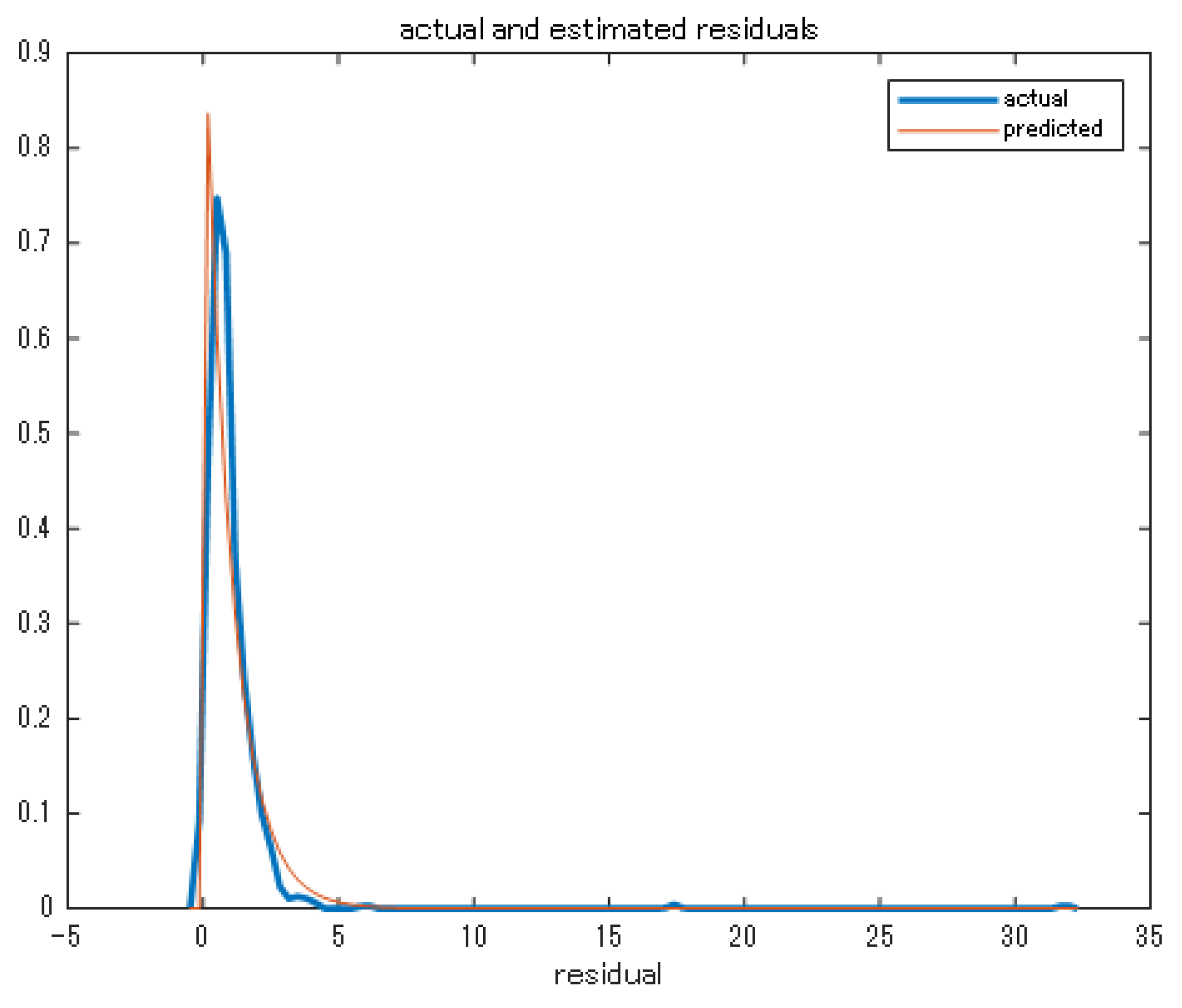
Figure 1 plots the distribution of the normalized sealed-bid residuals in our sample (defined as along with the distribution predicted by our fitted model. As shown, the assumption of a Weibull distribution provides a reasonable fit to the observed distribution of bids.
Next, we calculate the pseudo costs and of each auction described in Equations (6) and (7) using the estimated bid distributions to recover the cost distributions. We first calculate the pseudo costs and for each observed auction. The average values of the obtained and across the observed bids are and , respectively (We exclude auctions with negative pseudo costs from these calculations. We calculate negative pseudo cost for auctions with very high peak power, and thus it seems that our model does not fit auctions with very high peak power). The reason for the average pseudo cost of the incumbent being higher than that of the PPSs for observed auctions may be because the incumbent has systematically higher costs, or the PPSs tend to enter less costly auctions. To obtain the cost distributions, we simulate 5000 bids for the two types of bidders for a given auction characteristic using the estimated bid distributions. We obtain the implied pseudo costs and for each simulated bid, and plot them to obtain the cost distributions. Figure 2 plots the density functions of the costs of the incumbent and PPS firms for an auction with the median covariates (the peak power is 1287 kW, the load factor is and the year is , without and with bundling. The top figure is for the ordinary auction while the bottom one is for the bundled auction. The mean values of the cost distributions for the incumbent are and , without and with bundling, respectively. Those for the PPS are and respectively. The standard deviations of the cost distributions for the incumbent are and , without and with bundling, respectively. Those for the PPS are and respectively. Therefore, the PPS firms tend to have lower costs with greater dispersion than does the incumbent. Furthermore, bundled contracts are relatively more costly and costs are narrowly distributed for both types. Such an effect is somewhat larger for the incumbent, and we can then well appreciate that bundling seems to increase the asymmetry between the incumbent and the PPSs.
We should note that here we compare the artificially created auctions of the same scale with and without bundling, i.e., the total size of the bundled contracts is identical to the counterpart auction without bundling. The current analysis then shows that if a firm wins an auction that bundles several contracts, cost is higher and the cost distribution narrower. The cost may be higher because the firm needs to supply electricity for distinct locations, but the cost distribution may be narrower because the uncertainty of each contract may cancel each other out with multiple contracts. We refer to this as “the bundling effect”. In practice, however, bundling several contracts naturally makes the auction size larger, and there will be a scale effect in addition to the bundling effect. Such a case is of more interest and investigated later.
4.3. Estimation Results of Participation Model
Next, we estimate the participation of PPS firms. We assume that the parameter of the exponential function in Equation (11) depends on the load factor, the logarithm of peak power, the bundle dummy, and the year dummy. The number of PPS firms we observe in our data is 8. However, three of these participate in auctions only a few times. Therefore, we assume these firms are fringe bidders and that the main PPS firms do not consider the participation of these three firms when they make their own participation decision. Therefore, we set and to be the number of main PPS firms participating in an auction (therefore, n is the number of main PPS firms plus one). Table 3 shows the result of the maximum likelihood estimation of Equation (12). We can see that the higher the load factor, the lower the participation rate of PPS firms. We can also see that the higher the peak power, the more likely PPS firms will enter an auction. The coefficient on the bundle dummy is negative. This means, given the same size and load factor of an auction, if the auction bundles several contracts for various locations, PPS firms are less likely to take part in the auction. The estimated participation rate of PPS firms in an auction with the median covariates is for ordinal auctions and for bundled auctions.
To compute the ex ante expected profit of the function (9), we first need to obtain the expected profit given the number of participants or . To compute this, we repeatedly simulate the outcomes of auctions with the given covariates for a given number of participants. In a given simulation, we draw a bid for each bidder from the estimated bid distributions and obtain the corresponding pseudo costs for each bidder. We can then identify the auction winner and the realized bidder profits. We simulate 5000 auctions for each number of participants (from 2 to 6) to compute the expected profit given the number of participants for each bidder (hereafter we refer to this as the ex post profit). Then, following the function (9), we calculate the ex ante expected profit of a PPS firm from participating in the auction, given the auction and bundling characteristics, using the predicted probability for each number of participants. The ex ante expected profit of a PPS firm for an auction with median covariates is yen/kWh. If it is a bundled auction, the ex ante expected profit of a PPS firm is yen/kWh. Although the ex post expected profit is higher in the ordinary auction for any given number of participants, the differences in ex ante expected profit between the ordinary and the bundled auctions are not very great. This is because we expect the number of participants to be lower in the bundled auction and the ex post expected profit will be higher for a lower number of participants. These calculated ex ante profits are a sort of threshold profit for PPS firms in that they represent the profit to which PPS firms are indifferent between entering and not entering the auction.
5. Counterfactual Analyses
5.1. Unbundling the Actual Auction
In the previous sections, we have seen that given the same covariates, bundling raises the cost of bidders and reduces the participation rate of PPSs. A more practical question is, however, what would happen if we bundled several contracts and auction them together rather than auction these contracts separately. To answer this question, we need to consider the scale effect from bundling because bundling several contracts naturally increases the size of the contract (compared with independent contracts if sold separately). This increase in size will induce the greater participation of PPSs and reduce the costs of bidders. Therefore, the scale effect may offset the bundling effect and we need to investigate which effect potentially dominates.
To see the net effect of bundling, we investigate the auction in 2006 that procured electricity from 17 different places with 17 contracts altogether. The auctioneer is the Legal Affairs Bureau, with 17 contracts to procure electricity for 17 different branch offices auctioned together. We identify the size of each of the 17 contracts in the bundled auction. The size varies from 56 to 286 kW and the total size of the bundled auction is 1830 kW as shown in the second column in Table 4. We investigate what would have been the auction outcomes if these 17 contracts had been auctioned separately in individual auctions. We simulate auctions for the sizes of the 17 individual contracts to obtain the counterfactual expected payments of auctioneers, the costs of firms, the profits of winners, and the number of participants and compare these outcomes with the actual outcome when 17 contracts are bundled and auctioned together.
For each of the 17 contracts, we repeatedly simulate the outcomes of auctions for a given number of auction participants from 2 to In a given simulation, we draw a bid of each bidder from the estimated bid distributions in the previous section and obtain the corresponding cost values for each bidder. Then we can identify the auction winner and the realized bidder profits. We simulate 5000 auctions for each number of bidders to compute the ex post (of entry) expected profit of the winner, the payment of the auctioneer (the winning bid), and the cost of each type of firm. We then calculate the ex ante expected values of these auction outcomes using the probability of the number of participants. The probability of the number of participants is predicted by the estimation outcome of the probability rate (11) for each, given auction covariates of the 17 contracts. Because the PPS uses the mixed strategy with a probability less than one, the probability of no PPS entering an auction is not zero. When no PPS enters, the incumbent is the only bidder. We assume that in such a case the incumbent would bid exactly equal to the reserve price. As we do not observe the reserve price, we estimate it by regressing the incumbent’s bids on the logarithm of peak power, the load factor, and the bundle and year dummies using the data for auctions where the incumbent is the sole bidder, and obtaining the fitted values for each of the 17 contracts. We use these values as the expected payment of the auctioneer or the winning bid when the incumbent is the sole bidder. The expected number of participants is also calculated by the predicted probability rate (11) and shown in column 3. We also check whether the participant with the lowest cost (among the actual participants) wins an auction and calculate the expected value of this efficiency rate in column 8.
Table 4 provides the expected outcomes of the counterfactual 17 individual auctions from the simulation. Row 18 shows the weighted average of the outcomes of the 17 auctions. We also simulate the bundled auction to compare the expected values of the individual and bundled auctions in addition to comparing the expected value of the individual auctions and the actual (observed) value of the bundled auction. The expected outcome of the bundled auction is shown in row 19. The last row shows the actual observed outcome of the bundled auction. By comparing the weighted average of the 17 individual auctions and the bundled auction, we confirm that bundling reduces competition by slightly decreasing the number of PPS participants. The expected number of individual auctions is 2.346 while that of the bundled auction is 2.265, whereas the actual observed number of participants in the bundled auction is 2. However, the PPS that entered this auction was actually a fringe bidder that we did not take into account in the model. Therefore, the actual number of main PPSs that participated in this auction was zero.
We can also see that by bundling, the costs of both types of firms decrease. The expected costs of the incumbent are 15.114 yen/kWh for individual auctions and 14.905 yen/kWh for the bundled auction. Similarly, the expected costs for the PPSs are 14.366 yen/kWh for individual auctions and 13.990 yen/kWh for the bundled auction. However, this fall in costs does not seem to benefit firms, as we can see that the expected profit of the winner is much lower in the bundled auction. There are two possible reasons for the lower profit in the bundled auction. One is the greater asymmetry between the incumbent and the PPSs in the bundled auction. If asymmetry increases, weaker bidders bid more aggressively and are likely to win in auctions, leading to lower profits for the winners. However, as we can see in the last column in Table 4, the firms with the lowest costs almost always win both individual and bundled auctions in our case. Therefore, the increased asymmetry is unlikely to be the reason for the lower profit in the bundled auction. The second possible reason is the narrower distribution of costs in the bundled auction. According to theory, when the dispersion of the distribution of the costs of the other bidders becomes narrower, bidders tend to bid more aggressively. Although we did not present this in the table, the standard deviation of costs is much smaller in the bundled auctions. Therefore, it is likely that the expected profit of the winner is lower in the bundled auction because the opponent’s costs in these auctions are more predictable.
Given the lower costs and more aggressive strategies, the expected payment of the auctioneer is smaller in the bundled auction. The auctioneer seems to have conserved payment in these by bundling the 17 contracts together in an auction. The actual payment was 15.860 yen/kWh, which is close to the expected payment of 15.329 yen/kWh.
In any case, we see that the bundling effect dominates the scale effect in terms of participation, but the latter dominates the former in terms of the cost of firms. Although this case represented quite large bundling in that it bundles 17 small contracts together making for a medium-sized contract, it seems difficult to offset the bundling effect in participation entirely by the scale effect. However, bundling benefited the auctioneer in terms of payment at the expense of firms that needed to play more aggressive strategies.
5.2. Hypothetical Bundling
In the previous exercise, we saw that the bundling effect dominates the scale effect in terms of participation. However, in the expected term, the auctioneer has saved more payments than if it had auctioned the 17 contracts separately. In this subsection, we simulate hypothetical bundling to investigate when the scale effect dominates the bundling effect in terms of both the participation and costs of firms. Here we investigate two specific cases to see whether the scale effect dominates the bundling effect. In the first case, we select an auction in 2005 with a median-sized contract. Its peak power is 1287 kW and the load factor is 0.169. We then split the contract into three (that is, 429 kW each) without changing covariates other than the peak power, and compare the auction outcome of procuring electricity through three individual small contracts with the outcome of the original auction. In the second case, we select an auction in 2004 in the upper quantile of size. Its peak power is 2500 kW and the load factor is 0.168. We then split the contract into ten smaller contracts (that is, the peak power of each smaller individual contract is 250 kW) without changing the other covariates and compare the auction outcome with the outcome of the original auction. Like the previous subsection, we simulate 5000 auctions for a given number of participants to obtain the ex post expected auction outcomes and calculate ex ante expected outcomes, for both individual and bundled auctions for each case.
Table 5 and Table 6 provide the outcomes of each exercise. In the first case shown in Table 5, the expected unit cost for the individual small auction is 12.205 yen/kWh for the incumbent and 11.433 yen/kWh for a PPS. The expected cost for the bundled larger auction is 12.590 yen/kWh for the incumbent and 11.735 yen/kWh for a PPS. Therefore, under this hypothetical circumstance, we can see that the bundling effect dominates in terms of the firms’ costs. These costs slightly increase with bundling for both types of firms. The probability of a PPS bidder’s mixed strategy is 0.323 in the individual auction and 0.212 in the bundled auction. As a result, the expected number of firms in the individual auction is 2.615 and higher than 2.062 in the bundled auction. Therefore, we can say that the bundling effect also dominates in terms of the PPS participation strategy. At the same time, the auctioneer’s expected payments increase through bundling from 12.922 yen/kWh to 13.345 yen/kWh and the expected profit of the winner decreases from 2.489 yen/kWh to 1.641 yen/kWh. In this simulation, bundling does not benefit either the bidders or the auctioneer. The reason for the lower profit may be, as described above, the lower dispersion of the distribution of opponent costs in the bundled auctions. Despite the decreased margin, the auctioneer’s payment increases in the bundled auction mainly due to the increased costs.
In the second case in Table 6, the expected unit costs in an individual auction are 12.538 yen/kWh and 11.928 yen/kWh for the incumbent and a PPS, respectively. Those in the bundled auction are 12.312 yen/kWh and 11.522 yen/kWh for the incumbent and a PPS, respectively. Therefore, we can see that the scale effect dominates the bundling effect for both the incumbent and a PPS. The probability rate of the PPSs’ mixed strategy in an individual auction is 0.351 and 0.305 in the bundled auction. As a result, the expected number of participants is 2.756 in an individual auction and higher than the 2.525 for the bundled auction. Although we expect the number of participants to be lower in the bundled auction, the expected profit of the winner is lower in the same auction mainly due to the narrower cost distributions (and as a result more aggressive bidding). The expected auctioneer’s payment is also lower in the bundled auction. This is likely a reflection of the lower costs and more aggressive bidding of firms. This exercise turns out to provide a very similar result as the case in Section 5.1. in that the scale effect lowers the costs of firms, but scarcely dominates the impact of the bundling effect on participation of PPSs.
From these two exercises, we confirm that auctioneers benefit from bundling if it involves bundling many small contracts into a decently generous size due to the scale effect. In any case, bundling tends to reduce the number of PPSs participating despite the larger size, and so the probability of the incumbent winning is higher. Even in a case where the auctioneer’s payment is reduced through bundling, a benefit for the auctioneer arises partially at the cost of the bidders reducing the profit.
6. Conclusions
Electricity procurement auctions by public agencies in Tokyo began with the wave of deregulation in the retail electricity market in 2000. After several years of these auctions taking place, we observe the increasingly frequent practice of some public agencies bundling several contracts together in the one auction when purchasing electricity. We model these procurement auctions by including elements of asymmetry between the incumbent (the former monopolist) and the PPSs (new entrant firms) and endogenous participation to investigate the effects of bundling on the costs of firms, competition between the incumbent and the PPSs, and auction outcomes.
We find that bundling several contracts increases firm costs and reduces the dispersion of the distribution of costs. Bundling also tends to exclude PPSs, likely because of the difficulty arising in distributing electricity to distinct places. We find the negative effect increasing the costs of firms is somewhat mitigated by a larger scale of bundling, but that the negative effect on participation is scarcely offset by scale, and the number of participants is consistently lower in bundled auctions across all scenarios of our counterfactual situations. Because of the exclusion of the PPSs, the probability of an incumbent winning is higher in bundled auctions. The payment of the auctioneer may decline if bundling results in a large sized auction, but the profit of the winner is always lower in bundled auctions, presumably because firms bid more aggressively owing to the smaller dispersion of the opponents’ cost distributions.
Our current static analyses show that unless bundling results in decently larger size of auction, it harms the market by both increasing the payment of auctioneers and reducing the profit of the auction winner. It also distorts competition by excluding PPSs from the market. Furthermore, in a more dynamic context, the increasing practice of bundling contracts in auctions may harm the competitiveness of the PPSs by reducing their experience of auctions, as suggested in Olivares et al. [5] and this may eventually worsen the auction outcomes even more. The current and future lost trade between the auctioneer and PPSs given lost competitiveness should then be counted toward the competitive fairness loss à la Yano [7] and can threaten market quality. To see this effect more accurately, however, we would need to formulate a dynamic model for auctions in our next research step.
Funding
This research was funded by the Grant-in-Aid for Scientific Research (KAKENHI #15H03346).
Institutional Review Board Statement
Not applicable.
Informed Consent Statement
Not applicable.
Data Availability Statement
The data presented in this study are available on request from the corresponding author.
Acknowledgments
I would like to thank the editor, Makoto Yano and the three anonymous referees. I am also thankful Makoto Hanazono, Jun Nakabayashi, Takeshi Nishimura, Ryuji Sano and the participants at Workshop on Procurement, Auctions, and Mechanism Design in 2019 for their useful comments.
Conflicts of Interest
The author declares no conflict of interest.
Abbreviations
The following abbreviations are used in this manuscript:
| EPCo | Electric power company |
| IPV | Independent private value |
| JPEX | Japan electric power exchange |
| PPS | Power producer and supplier |
References
- Varian, H.R. Intermediate Microeconomics: A Modern Approach, 6th ed.; W W Norton & Co Inc.: New York, NY, USA, 2003; pp. 449–451. [Google Scholar]
- Bakos, Y.; Brynjolfsson, E. Bundling information goods: Pricing, profits, and efficiency. Manag. Sci. 1999, 45, 1613–1630. [Google Scholar] [CrossRef] [Green Version]
- Chernomaz, K.; Levin, D. Efficiency and synergy in a multi-unit auction with and without package bidding: An experimental study. Games Econ. Behav. 2012, 76, 611–635. [Google Scholar] [CrossRef]
- Maskin, E.; Riley, J. Asymmetric auctions. Rev. Econ. Stud. 2000, 67, 413–438. [Google Scholar] [CrossRef]
- Olivares, M.; Weintraub, G.Y.; Epstein, R.; Yung, D. Combinatorial auctions for procurement: An empirical study of the Chilean school meals auctions. Manag. Sci. 2012, 58, 1458–1481. [Google Scholar] [CrossRef] [Green Version]
- Yano, M. The foundation of market quality economics. Jpn. Econ. Rev. 2009, 60, 1–32. [Google Scholar] [CrossRef] [Green Version]
- Yano, M. Market Quality Theory and the Coase Theorem in the Presence of Transaction Costs; RIETI Discussion Paper Series 19-E-037; RIETI: Tokyo, Japan, 2019. [Google Scholar]
- Palfrey, T. Bundling decisions by a multiproduct monopolist with incomplete information. Econometrica 1983, 51, 463–483. [Google Scholar] [CrossRef]
- Armstrong, M. Multi-object auctions. Rev. Econ. Stud. 2000, 67, 455–481. [Google Scholar] [CrossRef]
- Cantillon, E.; Pesendorfer, M. Combination Bidding in Multi-Unit Auctions; CEPR Discussion Paper 6083; CEPR: London, UK, 2007. [Google Scholar]
- Kim, S.W.; Olivares, M.; Weintraub, G.Y. Measuring the performance of large-scale combinatorial auctions: A structural estimation approach. Manag. Sci. 2014, 60, 1180–1201. [Google Scholar] [CrossRef]
- Suzuki, A. The effect of bundling several contracts on electricity procurement auctions. Waseda Glob. Forum 2018, 14, 23–39. [Google Scholar]
- Suzuki, A. An Empirical Analysis of Entrant and Incumbent Bidding in Electric Power Procurement Auctions. Waseda Glob. Forum 2010, 7, 385–404. [Google Scholar]
- Athey, S.; Levin, J.; Seira, E. Comparing open and sealed bid auctions: Evidence from timber auctions. Q. J. Econ. 2011, 126, 207–257. [Google Scholar] [CrossRef]
- Samuelson, W.F. Competitive bidding with entry costs. Econ. Lett. 1985, 17, 53–57. [Google Scholar] [CrossRef]
- McAfee, R.P.; McMillan, J. Auctions and bidding. J. Econ. Lit. 1987, 25, 699–738. [Google Scholar]
- Levin, D.; Smith, J.L. Equilibrium in auctions with entry. Am. Econ. Rev. 1994, 84, 585–599. [Google Scholar]
- Maskin, E.; Riley, J. Existence of equilibrium in sealed high bid auctions. Rev. Econ. Stud. 2000, 67, 439–454. [Google Scholar] [CrossRef]
- Guerre, E.; Perrigne, I.; Vuong, Q. Optimal nonparametric estimation of first price auctions. Econometrica 2000, 68, 525–574. [Google Scholar] [CrossRef]
- Flambard, V.; Perrigne, I. Asymmetry in procurement auctions: Evidence from snow removal contracts. Econ. J. 2006, 116, 1014–1036. [Google Scholar] [CrossRef]
- Li, T.; Zheng, X. Entry and competition effects in first price auctions: Theory and evidence from procurement auctions. Rev. Econ. Stud. 2009, 76, 1397–1429. [Google Scholar] [CrossRef] [Green Version]
- Krasnokutskaya, E.; Seim, K. Bid preference programs and participation in highway procurement auctions. Am. Rev. 2011, 101, 2653–2686. [Google Scholar] [CrossRef] [Green Version]
Figure 1.
Actual and estimated distribution of residuals.

Figure 2.
Cost densities of incumbent and PPS firms.


Table 1.
Summary statistics.
| Variable | # | Mean | Std. Dev. | Min | Max |
|---|---|---|---|---|---|
| Unit bid | 546 | 18.438 | 14.972 | 9.890 | 188.410 |
| Unit bid (incumbent) | 189 | 19.771 | 20.319 | 10.05 | 188.41 |
| Unit bid (PPS) | 357 | 17.732 | 11.121 | 9.89 | 102.49 |
| Unit winning bid | 176 | 16.774 | 9.922 | 9.890 | 89.090 |
| # of participants | 190 | 3.326 | 1.199 | 2.000 | 7.000 |
| Peak power (kW) | 190 | 2073.016 | 2057.27 | 17 | 11,000 |
| Loadfactor | 190 | 0.113 | 0.059 | 0.002 | 0.263 |
| Incumbent win | 190 | 0.258 | 03439 | 0 | 1 |
| Bundling | 190 | 0.042 | 0.201 | 0 | 1 |
Table 2.
Estimation result of bid distribution.
| Coefficient | s.e. | |
|---|---|---|
| function | ||
| Constant | −171.289 | 12.1731 |
| # of bidders | −0.110 | 0.059 |
| Load factor | −10.398 | 20.952 |
| Load factor^2 | 13.595 | 69.391 |
| 1/load factor | 0.477 | 0.060 |
| ln(kw) | −1.325 | 0.730 |
| ln(kw)^2 | 0.044 | 0.048 |
| Bundle dummy | −4.443 | 2.204 |
| Bundle*ln(kw) | 0.629 | 0.310 |
| Incumbent dummy | 0.234 | 0.094 |
| Year dummy | yes | |
| function | ||
| Constant | 9.902 | 1.315 |
| Bundle dummy | 75.776 | 26.784 |
| Bundle*ln(kw) | −9.008 | 2.938 |
Table 3.
Estimation result of PPS participation.
| Coefficient | s.e. | |
|---|---|---|
| constant | 4371.104 | 1315.754 |
| load factor | −5.569 | 1.422 |
| ln(kw) | 0.272 | 0.094 |
| Bundle dummy | −0.857 | 0.416 |
| Year dummy | Yes | |
Table 4.
The effect of unbundling the actual auction.
| Contract ID | kW | Ex # of | Ex Cost of | Ex Cost of | Ex Payment of | Ex Profit of | Ex Efficiency |
|---|---|---|---|---|---|---|---|
| Participants | Incumbent | PPS | Auctioneer’s | Winner | |||
| 1 | 128 | 2.364 | 15.130 | 14.267 | 16.128 | 2.959 | 0.989 |
| 2 | 92 | 2.268 | 15.155 | 14.488 | 16.391 | 3.054 | 0.991 |
| 3 | 130 | 2.369 | 15.021 | 14.286 | 16.093 | 3.010 | 0.991 |
| 4 | 61 | 2.155 | 15.481 | 14.782 | 16.747 | 2.988 | 0.990 |
| 5 | 109 | 2.317 | 15.198 | 14.382 | 16.253 | 2.993 | 0.992 |
| 6 | 77 | 2.218 | 15.268 | 14.610 | 16.535 | 3.044 | 0.991 |
| 7 | 83 | 2.239 | 15.160 | 14.559 | 16.475 | 3.029 | 0.992 |
| 8 | 117 | 2.337 | 15.151 | 14.325 | 16.201 | 2.955 | 0.989 |
| 9 | 286 | 2.616 | 14.664 | 13.984 | 15.500 | 2.828 | 0.990 |
| 10 | 109 | 2.317 | 15.156 | 14.443 | 16.262 | 2.961 | 0.991 |
| 11 | 125 | 2.357 | 15.053 | 14.325 | 16.141 | 3.000 | 0.991 |
| 12 | 63 | 2.163 | 15.421 | 14.655 | 16.698 | 3.054 | 0.990 |
| 13 | 70 | 2.192 | 15.445 | 14.613 | 16.609 | 3.029 | 0.991 |
| 14 | 56 | 2.132 | 15.496 | 14.728 | 16.791 | 3.060 | 0.991 |
| 15 | 169 | 2.448 | 14.934 | 14.202 | 15.908 | 2.920 | 0.990 |
| 16 | 76 | 2.214 | 15.359 | 14.545 | 16.546 | 3.060 | 0.992 |
| 17 | 57 | 2.137 | 15.568 | 14.707 | 16.782 | 3.0303 | 0.990 |
| Weighted average | 2.346 | 15.114 | 14.366 | 16.192 | 2.971 | 0.991 | |
| Bundled | 1830 | 2.265 | 14.905 | 13.990 | 15.329 | 1.661 | 0.982 |
| Observed | 1830 | 2 | 15.860 |
Table 5.
Expected values for independent vs. bundled auctions (case 1).
| Cost | Cost | # of | Payment | Prob of | Profit of | Efficiency | |
|---|---|---|---|---|---|---|---|
| (Incumbent) | (PPS) | Participants | Incumbent Win | Winner | |||
| Independent | 12.205 | 11.433 | 2.615 | 12.922 | 0.421 | 2.489 | 0.987 |
| Bundled | 12.590 | 11.735 | 2.062 | 13.345 | 0.532 | 1.641 | 0.969 |
Table 6.
Expected values for independent vs. bundled auctions (case 2).
| Cost | Cost | # of | Payment | Prob of | Profit of | Efficiency | |
|---|---|---|---|---|---|---|---|
| (Incumbent) | (PPS) | Participants | Incumbent Win | Winner | |||
| Independent | 12.538 | 11.928 | 2.756 | 13.202 | 0.402 | 2.4736 | 0.988 |
| Bundled | 12.312 | 11.522 | 2.525 | 12.750 | 0.426 | 1.6865 | 0.977 |
Publisher’s Note: MDPI stays neutral with regard to jurisdictional claims in published maps and institutional affiliations. |
© 2021 by the author. Licensee MDPI, Basel, Switzerland. This article is an open access article distributed under the terms and conditions of the Creative Commons Attribution (CC BY) license (https://creativecommons.org/licenses/by/4.0/).
Share and Cite
MDPI and ACS Style
Suzuki, A. Investigating Pure Bundling in Japan’s Electricity Procurement Auctions. Mathematics 2021, 9, 1622. https://0-doi-org.brum.beds.ac.uk/10.3390/math9141622
AMA Style
Suzuki A. Investigating Pure Bundling in Japan’s Electricity Procurement Auctions. Mathematics. 2021; 9(14):1622. https://0-doi-org.brum.beds.ac.uk/10.3390/math9141622
Chicago/Turabian StyleSuzuki, Ayako. 2021. "Investigating Pure Bundling in Japan’s Electricity Procurement Auctions" Mathematics 9, no. 14: 1622. https://0-doi-org.brum.beds.ac.uk/10.3390/math9141622
Note that from the first issue of 2016, this journal uses article numbers instead of page numbers. See further details here.