An Enhanced Evolutionary Software Defect Prediction Method Using Island Moth Flame Optimization

Abstract

Software defect prediction (SDP) is crucial in the early stages of defect-free software development before testing operations take place. Effective SDP can help test managers locate defects and defect-prone software modules. This facilitates the allocation of limited software quality assurance resources optimally and economically. Feature selection (FS) is a complicated problem with a polynomial time complexity. For a dataset with N features, the complete search space has $2^N$ feature subsets, which means that the algorithm needs an exponential running time to traverse all these feature subsets. Swarm intelligence algorithms have shown impressive performance in mitigating the FS problem and reducing the running time. The moth flame optimization (MFO) algorithm is a well-known swarm intelligence algorithm that has been used widely and proven its capability in solving various optimization problems. An efficient binary variant of MFO (BMFO) is proposed in this paper by using the island BMFO (IsBMFO) model. IsBMFO divides the solutions in the population into a set of sub-populations named islands. Each island is treated independently using a variant of BMFO. To increase the diversification capability of the algorithm, a migration step is performed after a specific number of iterations to exchange the solutions between islands. Twenty-one public software datasets are used for evaluating the proposed method. The results of the experiments show that FS using IsBMFO improves the classification results. IsBMFO followed by support vector machine (SVM) classification is the best model for the SDP problem over other compared models, with an average G-mean of 78%.

1. Introduction

The software industry has recently undergone further development in various aspects related to the software development life-cycle (SDLC). An important aspect to achieve during SDLC is reliability and error-free code. Software defect describes the error status that occurs at the program or system level which leads to erroneous results and unexpected actions and allows the system to behave in an unintended way [1]. There are several reasons behind software defects [2] such as incomplete or ambiguous requirements due to miscommunication and misinterpretation during requirements elicitation, errors in assumptions and preliminary specifications, lack of knowledge in the domain, developers with insufficient practical experience and technical skills, poor programming logic, and so forth. Software defects have many negative consequences for the quality of the software and the overall effectiveness of the system in terms of time, budget, risks, and resources [3]. For example, errors in the design stage may require a high cost of maintenance and restructuring. Poor quality software production will not satisfy customer requirements and will ultimately affect the company’s reputation [4].

Defect prediction plays an important role in identifying error-prone modules and controlling the percentage of defects in the software, which improves the quality of the software. This will improve the testing process as it will focus on parts that are more likely to work incorrectly [5]. On the other hand, the distribution of errors in the code determines the refactoring candidates, which enhances the quality and the efficiency of the software product [6,7]. There are three categories of software defect prediction (SDP): prediction of the number of defects, prediction of the severity of defects, and prediction of whether the software module is defective or not. Among them, the last category is the most frequently used, where the SDP is formulated as a binary classification problem that deals with two classes called defect and non-defect [8].

In the literature, many machine learning algorithms have been proposed to predict software defects either through supervised or unsupervised learning [9,10,11,12,13,14]. Supervised learning is the most common machine learning method used to create SDP models, where the applied learning strategy is based on inferring a pattern from a set of instances (training data set). This pattern can then be applied to invisible instances (testing data set) to predict their class labels. Examples of supervised data mining methods used to reliably solve the software defects problem include decision trees (DT), artificial neural network (ANN), naïve Bayesian (NB), support vector machine (SVM), and random forest (RF) [15].

Feature selection (FS) is a data mining step to select the most informative features in the dataset. Its main target is to obtain a feature subset with a minimum length that, at the same time, achieves the maximum classification performance [16]. The FS process consists of search and evaluation sub-processes. The evaluation sub-process utilizes the dataset characteristics (e.g., filters) or classifier (e.g., wrappers) to evaluate a feature subset [17]. For applying the search in the FS process, many methods can be performed. Traditionally, brute force methods have been applied, but they are time-consuming. These are complete search methods because they generate the entire feature space and traverse all the feature subsets. Meta-heuristic methods such as swarm intelligence [18] algorithms generate random solutions and achieve promising results within less time [19]. Swarm intelligence methods have been used widely for enhancing the FS process, such as face recognition [20], machine scheduling [21], medical diagnosis [17,22], multi-objective power scheduling [23] and software defect prediction [24].

The moth flame optimization (MFO) algorithm is a swarm intelligence algorithm that is commonly used in many applications [25,26,27]. MFO generates a swarm of solutions to explore the search space. Furthermore, it adopts a spiral method to update the positions of moths and change their positions. The gradual degradation of the number of solutions improves the exploration/exploitation trade-offs. This supports the adaptive convergence behavior of the algorithm. However, MFO inherits the drawbacks of swarm intelligence algorithms, such as stagnation in local minima and premature convergence. To address these shortcomings, the improvement of the MFO algorithm has been proposed [28,29,30,31].

The island-based model has been integrated with many swarm intelligence algorithms. In this model, the members of the population are distributed among a set of sub-populations where they are managed separately using local rules. In a migration step, migrants interact with each other. Usually, this is done by exchanging the highly fit solutions between islands. This step increases the diversity among solutions and enhances the convergence trends. Three main factors affect the performance of the migration: the rate, the frequency, and the topology of migration. The rate of migration determines the number of exchanged solutions between islands. The frequency of migration indicates the number of invocations for the migration process. Lastly, the topology of migration defines the way the solutions are exchanged between islands. In the literature, there are many studies that integrate the island models with metaheuristic algorithms [32,33,34,35].

This paper proposes the island model to enhance the binary MFO (BMFO) algorithm. The new variant named IsBMFO is used to enhance the FS process and the prediction of software defects. The main objectives are enhancing the diversity of the solutions, alleviating the local minima problem, and enhancing convergence trends. The islands are generated from dividing the population into a group of islands. Each island consists of a group of solutions. Solutions are enhanced locally in each island, and then they are exchanged using a migration mechanism that adopts a random-ring topology. This topology exchanges the solution with the worst fitness in the destination island with the solution with the best fitness from the source island.

The remaining parts of this paper are arranged into sections as follows: Section 2 discusses related studies in the literature. Section 3 provides background about the applied classifiers, the MFO algorithm, and the island model. Section 4 describes the IsBMFO. Section 5 describes the experiments and the related discussions. Finally, Section 6 draws the conclusions of the paper and suggests some possible future works.

2. Related Works

Recently, the SDP problem has become a noteworthy research topic that has increasingly attracted the interest of researchers. Several methods from statistics, information theory, and machine learning fields have been used to predict defected models and reduce the cost of software production and maintenance [36,37].

In [38], the authors aimed to find the count of defects when the software process is not properly executed. For the classification of defects, the authors employed different DT algorithms such as C4.5 and ID3. Pattern mining methods were used to evaluate the defect patterns.

Can et al. [39] proposed a prediction model for software defects using particle swarm optimization (PSO) and SVM called the P-SVM. Specifically, the PSO was used for the optimization of parameters of the SVM. After identifying the optimal parameters of the SVM, it was used to predict the defects in the software. The experiments were performed over the JM1 dataset. P-SVM was compared with the SVM model, back propagation neural network (BPNN) model, and optimized SVM using the genetic algorithm (SVM-GA) model. The results proved the superiority of the P-SVM model.

Shuai et al. [40] proposed a cost-sensitive SVM (CSSVM) model which is based on dynamic SVM using the concept of cost-sensitivity. The model was optimized using the GA algorithm. The fitness function used the geometric accuracy metric. The results of the experiments showed that the GA-CSSVM achieved a higher area under the curve (AUC) value, indicating better prediction accuracy.

Agrawal and Tumar [41] proposed an FS approach based on a linear twin SVM (LTSVM) classifier to predict the defective software modules. They worked on determining the most important metrics set. The reduced metrics set, obtained after the FS process, was used to enhance the predictive power of their approach. The experiments on four PROMISE datasets showed the effectiveness of the LSTVM model.

In [42], the authors studied the software defect prediction using different methods such as DT, decision tables, RF, NN, NB, artificial immune recognition system, CLONALG, and Immunos. They used four software datasets from NASA. Principal component analysis (PCA) and correlation-based FS methods were applied for evaluation. The experiments proved that RF is the best predictor for large datasets while NP is the best predictor for small datasets. Moreover, the experiments showed that the Immunos-99 algorithm performed well when the FS method was applied, while the AIRSParallel algorithm performed better without applying FS methods.

Singh and Chung [15] applied common machine learning algorithms including artificial NN, PSO, DT, NB, and linear classifier. The authors used the KEEL tool and k-fold cross-validation method. The results on seven open-source NASA datasets proved the superiority of the linear classifier in terms of accuracy.

Recently, in [43], the authors used the oversampling technique SMOTE along with FS using PSO on object-oriented metrics. The obtained features were then utilized to train the datasets on SVM to predict defects. The experiments showed that SVM performed better when the dataset was balanced with SMOTE and PSO was used for selecting the feature set.

In [44], the authors studied the effect of 46 FS methods based on NB and DT classifiers over software defect datasets. The results proved that there is no model that can be considered the best FS method. This is because their performances depend on the applied classifiers, used evaluation metrics, and datasets.

Overall, in the literature, many studies used classification algorithms for classifying software defects datasets such as NB, KNN, C4.5, and SVM. Some of these studies proposed GA and PSO algorithms for optimizing the SVM. However, the number of works that addressed the problem of FS in the domain of software defect prediction is still few. This work focuses on identifying the features subset that is considered the optimal one for improving the efficiency of classifiers. Based on the no free lunch (NFL) theorem, no optimization algorithm is considered the best solution to solve every optimization problem. Hence, there is always room to develop, propose, and enhance optimization algorithms to tackle different optimization problems. MFO has remarkable proprieties among swarm intelligence algorithms. Therefore, in this study, we further enhance its performance to optimize FS and produce better results for software defect prediction.

3. Background

3.1. Classification Algorithms

3.1.1. K-Nearest Neighbor Classifier (k-NN)

This is a type of classification algorithm that belongs to a larger category of pattern recognition algorithms known as instance-based or lazy learning algorithms. Instead of conducting the generalization in an explicit training phase, they rely on computing the distance (similarities) between the unlabeled new query instance and its nearest k neighbors from the labeled training instances stored in memory. The basic idea for k-NN is that the nearby points in space are likely to have a similar class concept. In classification problems, the input to the k-NN is the k closest examples among the training examples, and the output is the labels of these examples. Assigning labels depends on the majority of votes obtained from the k closest neighbors for the required example. The comparison and the calculation of the closeness between points are done based on a predefined distance metric such as the Euclidean distance.

3.1.2. Support Vector Machines (SVM)

SVM is a supervised robust learning model that is based on a statistical learning framework. Given a set of training examples, the SVM maps these examples to one or the other category. This means that SVM is a binary classifier that applies an improbable linear method. The SVM tries to put the training examples in points in space in such a way to maximize the gap between the two categories. In addition, SVM can perform a non-linear classification using the kernel trick.

3.1.3. Naive Bayes Classifier (NB)

NB is a classification algorithm that applies the Bayes’ theorem, and it is considered a probabilistic classifier. NB assumes strong independence between features. NB gives the probability of membership of an example to each class. NB is among the simplest of Bayesian network models that can achieve higher classification results.

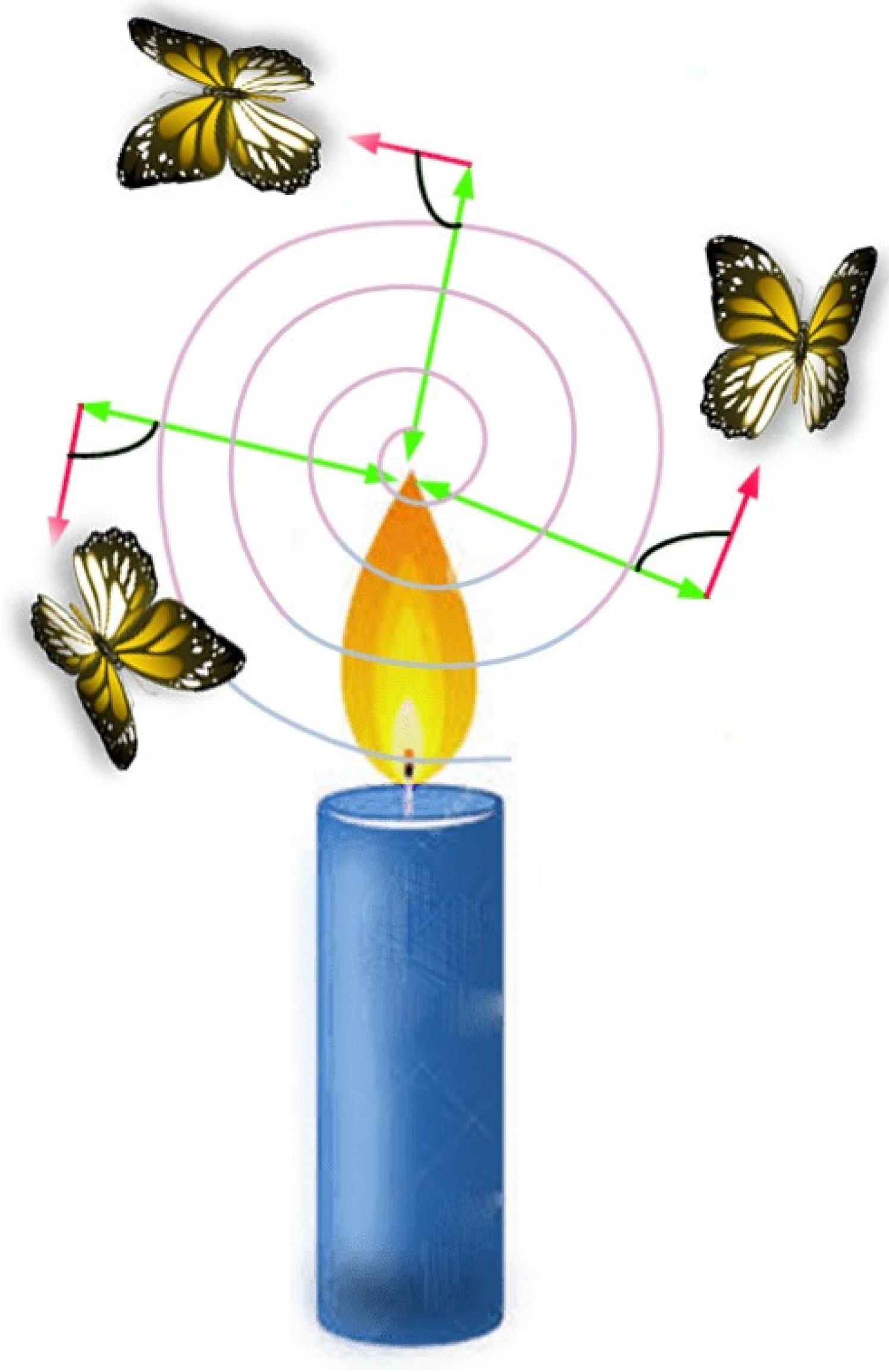
3.2. Overview of Moth Flame Optimization Algorithm

The moth flame optimization algorithm (MFO) is a widely applied swarm intelligence algorithm [45] with remarkable results. The inspiration of MFO is from an insect called a moth. Moths move straight in nature by following a natural mechanism called transverse orientation. This mechanism enables moths to go far distances straight by keeping the same angle with a distant source of light such as the moon. However, the transverse orientation does not work correctly when the source light is near the moths. Consequently, moths are forced to enter a spiral path and move around the light. Figure 1 shows the movement of moths around a candle by following a spiral path.

The MFO identifies a set of solutions (population) where the solutions are called moths. The moths represent the possible solutions to the optimization problem. A specified fitness function is used to determine the fitness of each moth. Another component of the MFO is the flame. Both a moth and a flame are solutions; they differ in their update strategy. Moths are the identified solutions that are candidates to be the best solutions, but flames are the best achieved solutions. Each flame is replaced whenever a better solution is found so that the best solutions are never missed.

The spiral movement of moths around the flames is formulated in Equation (1), which describes the movement of moths in a spiral path around a candle where $M{o}_i$ is the ith moth, $F{l}_j$ is the jth flame, and $Sp$ is the function of spiral path.

Equation (2) shows the logarithmic function used to formulate the spiral movement of moths, where $D{s}_i$ is the distance between the ith moth and the jth flame as shown in Equation (3), b is a constant value that determines the shape of the logarithmic spiral, and t is a random number in [−1, 1]. The parameter $t=-1$ represents the closest position of a moth to a flame, where $t=1$ represents the farthest position between a moth and a flame. To increase exploitation, the t parameter is selected in the range [r, 1], where r is decreased linearly across iterations from −1 to −2.

$$Moi=Sp(M{o}_i,F{l}_j)$$

(1)

$$Sp(M{o}_i,F{l}_j)=D{s}_i\times e^{bt}\times cos(2\Pi )+Flj$$

(2)

$$D{s}_i=|M{o}_i-F{l}_j|$$

(3)

Equation (4) shows the gradual decrease of the number of flames across the iterations, where $Ct$ is the current number of iterations, $Mfl$ is the maximum number of flames, and $Mt$ is the maximum number of iterations.

$$FlameNumber=round(Mfl-Ct\times (Mfl-1)/Mt)$$

(4)

3.3. Binary Moth Flame Optimization for Feature Selection

MFO was designed to solve continuous optimization problems. FS is a discrete problem in which the search space consists of two values, “0” or “1”. For this reason, MFO needs some modification to be able to optimize in a binary feature space. In [46], the authors used the transfer functions to produce a binary optimizer from the original continuous version of the optimizer. A mapping procedure is used to convert the continuous update process into a binary process. Thus, the elements of the updated solutions are either “0” or “1”.

In the proposed models, the sigmoid transfer function is used to produce a BMFO from the original MFO. The sigmoid function defines a probability for each element of the solution within a range [0, 1]. It was used in [47] to produce a binary variant of PSO. The velocity (step) is analogous to the first term of Equation (2) in the MFO algorithm. This term is redefined in Equation (5) as the probability for changing the position of moths. Each moth updates its position in the binary search space using Equation (7) based on the probability generated from Equation (6). Algorithm 1 shows the BMFO algorithm.

$$\Delta Mo=D{s}_i\times e^{bt}\times cos(2\Pi )$$

(5)

$$Trf(\Delta M{o}_t)=1/(1+e^{\Delta M{o}_t})$$

(6)

$$M{o}_i^d(t+1)=\left\{\begin{array}{cc}0,\hfill & \mathrm{if}rand<Trf(\Delta M{o}_{t+1})\hfill \\ 1,\hfill & \mathrm{if}rand⩾Trf(\Delta M{o}_{t+1})\hfill \end{array}\right.$$

(7)

Algorithm 1 The pseudo-code of BMFO.

Input: $Mt$, n (# moths), d (# dimensions) Output: near optimal moth Initialization process for the moths  while  $Ct\le Mt$  do   modify the number of flames using Equation (4)   FMo = Fitness(Mo);   if $Ct$ == 1 then    $Fl$ = $sort\left(Mo\right)$;    $FFl$ = $sort\left(FMo\right)$;   else    $Fl$ = $sort(M{o}_{Ct-1},M{o}_{Ct})$;    $FFl$ = $sort(FM{o}_{Ct-1},FM{o}_{Ct})$;   end if   for i = 1 : n do    for j = 1 : d do     Modify r and t;     Compute $Ds$ by Equation (3) based on the corresponding moth;     Modify the step vector of a moth $\Delta Mo$ using Equation (5).     Compute the probabilities by Equation (6).     Modify the position of a moth by Equation (7)    end for   end for   $Ct$ = $Ct$ + 1;  end while

The fitness function is formulated in Equation (8), where $Err$ is the error rate, $\left|Sf\right|$ is the number of selected features in the reduced data set, $\left|Cf\right|$ is the number of features in the original data set, and $\alpha \in [0,1]$, $\beta =(1-\alpha )$ are two parameters that indicate the significance of classification and the number of selected features according to [19].

$$Fitness=\alpha \times Err+\beta \times \frac{\left|Sf\right|}{\left|\mathsf{Cf}\right|}$$

(8)

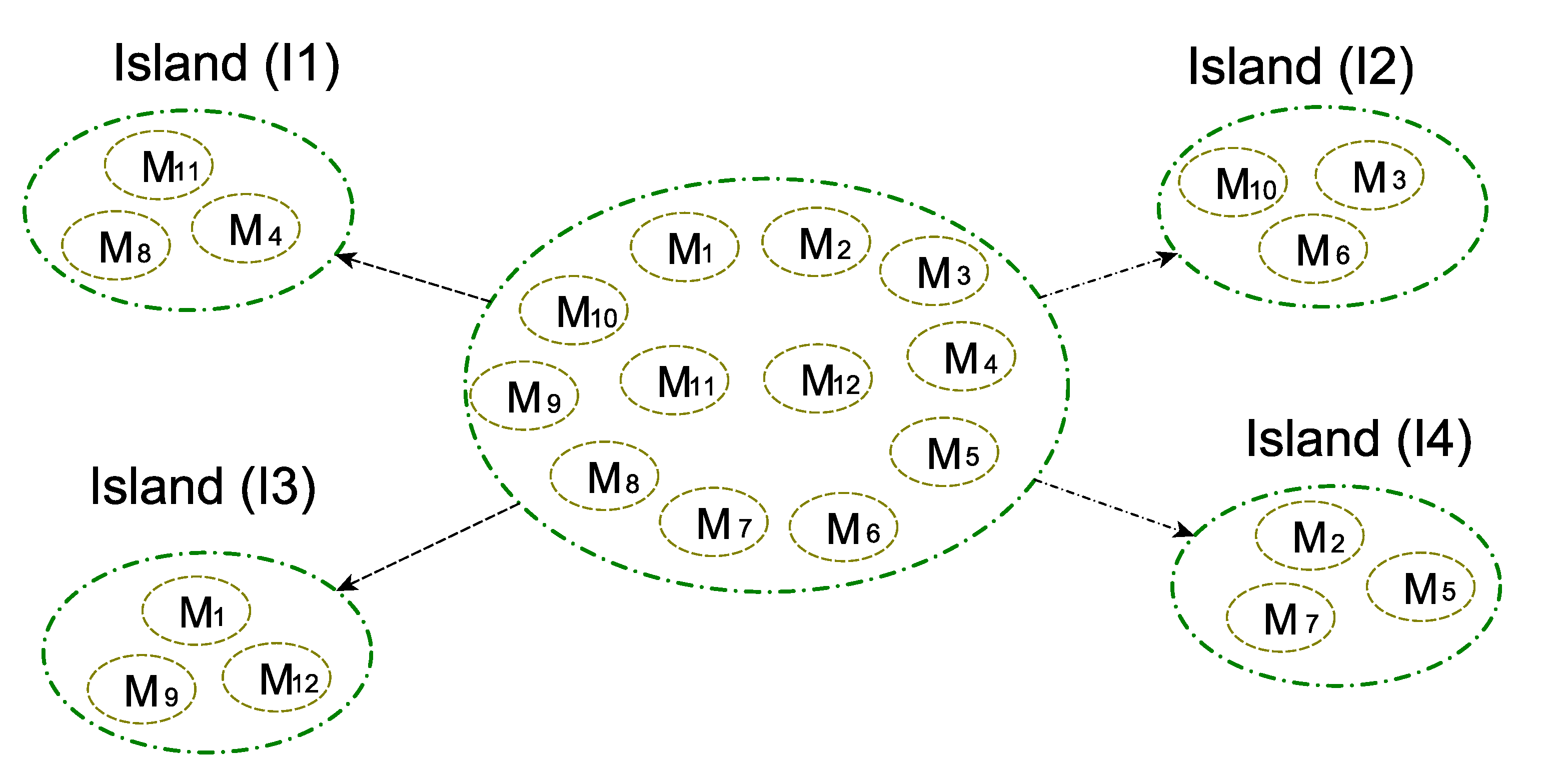
3.4. Fundamentals to Island-Based Model

The island model is an efficient method for structuring the population and increasing its heterogeneity [33,34]. This is applied by dividing the population into smaller sub-populations called (islands). The evolutionary algorithm is applied on each island either in a synchronous or asynchronous way. A migration process is applied after a period to allow solutions from different islands to exchange their positions. The exchange of solutions between islands improves exploration/exploitation trade-offs. This happens because the low-quality solutions with low-fitness values can approach the region where the global optima locate. Another advantage of the island model is that it enables the parallel implementation of the evolutionary algorithm on each island. This can minimize the computation time of complex optimization problems.

The island model has been applied with several evolutionary computation algorithms. The main purpose is to increase the population diversity and search the search space effectively. Examples of island-based models include the island differential evolution [48], island flower pollination algorithm [33], island ant colony [49], island bat algorithm [32], and island harmony search [34].

Several factors affect the island model such as the number of islands or the number of times the solutions are exchanged between islands. For integrating the island model with evolutionary algorithms, the partitioning and migration operators are used. Partitioning accounts for the number of islands ($I{s}_n$) and the size of the island ($I{s}_s$). In migration, the $M{r}_m\times I{s}_s$ moths are to be swapped between islands after a predetermined number of iterations $I{t}_m$, where $M{r}_m$ is the migration rate and $I{s}_s$ is the island size.

The migration process can be performed in a synchronous or asynchronous way. In the synchronous way, the solutions are swapped between islands simultaneously. The asynchronous way enables solutions to change their islands to other ones after a specific time. Therefore, the migration times are different between islands. An important factor in migration is the topology. There are two migration typologies: either static or dynamic. The static typologies determine the paths between islands, so they are not changeable. The dynamic typologies determine the paths between islands during the execution time. The effectiveness of the island model is also affected by the migration process. This indicates which solutions will be selected to migrate between islands. A common migration policy is known as best–worst. It selects the best solution (with the highest fitness value) from the source island to be swapped with the worst solution (with the lowest fitness value) from the destination island [48]. Another known policy for applying migration is random-random. It selects a random solution from the source island to be swapped with a random solution from the destination island [50].

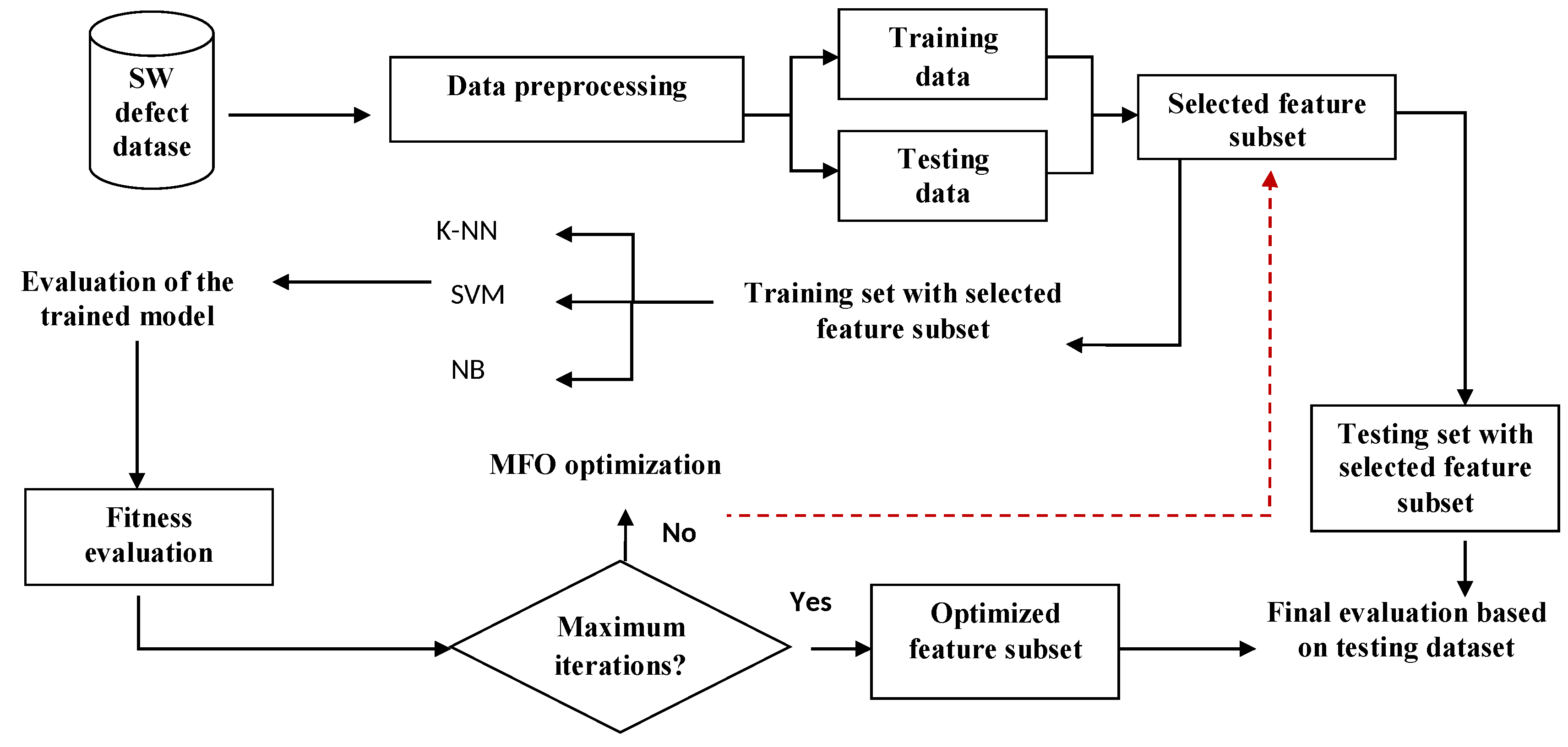
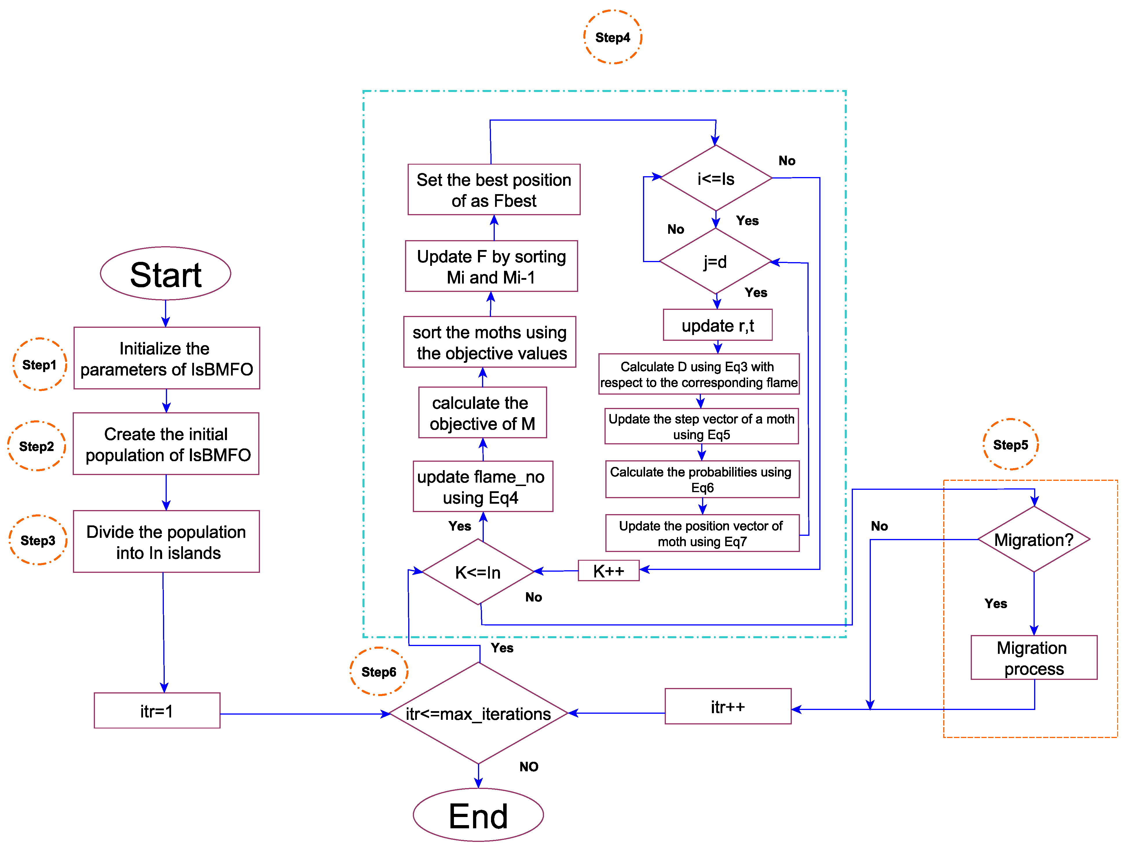
4. Island-Based MFO (IsMFO) Algorithm

This section proposes the island MFO algorithm. Figure 2 shows the overall methodology followed in this work. Initially, the population of moths is split into a set $I{s}_n$ islands of moths. Each island is of size $I{s}_s$ moths. The MFO runs independently and asynchronously on each island. The number of times the algorithm runs depends on the migration frequency $F{r}_m$. The moths are exchanged based on random-ring migration topology, and the number of moths to be exchanged depends on the migration rate $M{r}_m$. The migration policy used is the best–worst. This technique is applied more than one time until reaching the maximum iteration.

The IsBMFO flowchart is shown in Figure 3, and the pseudo-code is shown in Algorithm 2.

Algorithm 2: The IsBMFO pseudo-code.

————Identification of the IsBMFO parameters——————— Set the IsBMFO parameters $Mt$, n, d, $I{s}_n$, $I{s}_s$, $M{r}_m$, $F{r}_m$ ————Initialize the IsBMFO positions——————— Initialize the positions of moths 0: ———Split IsBMFO into a group of islands————————  Flag(y) = False, $\forall y=(1,2....n)$  for K = 1 : $I{s}_n$ do   for i = 1 : $I{s}_s$ do    select y, where y ∈ (1, 2, …, n)    while Flage( y) is true do     select y, where y ∈ 1, 2, …, $S_n$    end while    Add $x_y$ to island $I{s}_k$   end for  end for  while  $Ct\le Mt$  do   ——–Improvement step————————   for i = 1 : $I{s}_n$ do    Update flame no using Equation (4)    FMo = Fitness(Mo);    if $Ct$ == 1 then     $Fl$ = $sort\left(Mo\right)$;     $FFl$ = $sort\left(FMo\right)$;    else     $Fl$ = $sort(M{o}_{Ct-1},M{o}_{Ct})$;     $FFl$ = $sort(FM{o}_{Ct-1},FM{o}_{Ct})$;    end if    for i = 1 : Is do     for j = 1 : d do      Modify r and t;      Compute $Ds$ by Equation (3) based on the corresponding moth;      Modify the step vector of a moth $\Delta Mo$ by Equation (5).      Compute the probabilities by Equation (6).      Modify the position of a moth by Equation (7)     end for    end for   end for   ————— Migration of moths————   if t mod $F{r}_m$ = 0 then    for $y=1$, …, $I{s}_n$do     $k=1$     while$k\le M{r}_m\times Is$do      $xWorst(k,y+1)=xBest(k,y)$     end while    end for   end if   $Ct$ = $Ct$ + 1  end while

The IsBMFO steps are explained next:

Step 1: This is the initialization step for the BMFO parameters. These include the # dimensions (d), # moths (n), and the # iterations (#$Mt$). The fitness function $f\left(Mo\right)$ and the representation of a moth Mo = ($m{o}_1$, $m{o}_2$, …, $m{o}_d$ ) are also defined. The island model parameters should be identified as follows:

• Island number ($I{s}_n$): this determines the number of sub-populations that is less than or equal to n.
• The size of island ($I{s}_s$): the population size for each island can be computed using the formula $I{s}_s=n/I{s}_n$ since all islands are homogeneous.
• The frequency of migration ($F{r}_m$): this indicates the required iterations number to call the migration function.
• The rate of migration ($M{r}_m$): this indicates the number of moths swapped between islands based on $I{s}_s$, where $M{r}_m\times I{s}_s\le I{s}_s$.

Step 2: Identifies the solutions in the population of IsBMFO. In this step, IsBMFO follows the same process as in the MFO. The random moths are $Mo$ = ($m{o}_1,m{o}_2,...,m{o}_n$), and the fitness function (i.e., $f\left(mo\right)$) for each moth ($m{o}_j$, where $j\in (1,2,...,n))$ is computed.

Step 3: Split the IsBMFO population into a set of islands $I{s}_n$ of size $I{s}_s$ for each one as shown in Figure 4. The island vector is Is = ($I{s}_1$, $I{s}_2$, …, $I{s}_n$), where each variable $I{s}_j\in (1,2,...,I{s}_n)$. As an example, assume $I{s}_n$ = 4 and $I{s}_s$ = 3 are the division of IsBMFO population of size n = 12. Assume that $Is=$ (3, 4, 2, 1, 4, 2, 4, 1, 3, 2, 1, 3), then island $I{s}_1$ = ($M_4$, $M_8$, $M_{11}$), island $I{s}_2$ = ($M_3$, $M_6$, $M_{10}$), island $I{s}_3$ = ($M_1$, $M_9$, $M_{12}$), and island $I{s}_4$ = ($M_2$, $M_5$, $M_7$). Remember that each moth is assigned randomly to an island.

Step 4: The step of improvement includes updating the flames number, calculating the objective values of moths, and sorting of moths based on their fitness values. In this stage, the moth is updated based on the computed distance between a moth and the flame corresponding to it.

Step 5: Migration process of IsBMFO. The main target of the migration process is to exchange the moths between islands. After a predefined iteration number specified by ($F{r}_m$), the migration process is applied as shown in Algorithm 2. A specific number of moths are exchanged on each island based on the migration rate $M{r}_m$, where $M{r}_m\times I{s}_s\le I{s}_s$. The migration uses the best–worst policy and a random ring topology. The best–worst policy selects the best $M{r}_m\times I{s}_s$ moths from an island to replace the worst $M{r}_m\times I{s}_s$ moths on a neighboring island. In random-ring topology, the islands are rearranged in a random way to compose a ring $(I{s}_j,I{s}_{j+1},...,I{s}_k,I{s}_j)$ in which the island neighbor to $I{s}_j$ is island $I{s}_{j+1}$, and the island neighbor to $I{s}_{j+1}$ is island $I{s}_{j+2}$, etc.

5. Experimental Results

5.1. Model Evaluation Metrics

The basic evaluation metric that is used to evaluate the proposed software defect prediction algorithm is the confusion matrix.

Table 1. Confusion Matrix.

	Actual Labels
Predicted labels		Defect	Non-Defect
	Defect	TruePos	FalsePos
	Non-defect	FalseNeg	TrueNeg

shows the confusion matrix.

From the confusion metric, other evaluation metrics can be deduced, such as:

• Recall: The ratio of correctly classified defected instances, as in Equation (9):

  $$Recall=\frac{TruePos}{TruePos+FalseNeg}$$

  (9)
• Precision: The ratio of the correctly classified defected instances among the retrieved instances. It can be calculated by Equation (10):

  $$Precision=\frac{TruePos}{TruePos+FalsePos}$$

  (10)
• G-mean: The recall of each class, as in Equation (11):

  $$G-mean=\sqrt{\frac{TruePos}{TruePos+FalseNeg}\times \frac{TrueNeg}{FalsePos+TrueNeg}}$$

  (11)

5.2. Datasets Specifications

The methodology is verified by a series of 21 public benchmark software datasets.

Table 2. Description of datasets.

No.	Name	Features	Instances	Defects	Non-Defects	Defect Ratio	Non-Defect Ratio
D_1	cm1	38	327	42	285	12.8	87.2
D_2	jm1	22	7782	1672	6110	21.5	78.5
D_3	kc1	22	1183	314	869	26.5	73.5
D_4	kc3	40	194	36	158	18.6	81.4
D_5	mc1	39	1988	46	1942	2.3	97.7
D_6	mw1	38	253	27	226	10.7	89.3
D_7	pc1	38	705	61	644	8.7	91.3
D_8	pc2	37	745	16	729	2.1	97.9
D_9	pc3	38	1077	134	943	12.4	87.6
D_10	pc4	38	1287	177	1110	13.8	86.2
D_11	pc5	39	1711	471	1240	27.5	72.5
D_12	ant-1.7	21	745	166	579	22.3	77.7
D_13	camel-1.6	21	965	188	777	19.5	80.5
D_14	ivy-2.0	21	352	40	312	11.4	88.6
D_15	jedit-4.3	21	492	11	481	2.2	97.8
D_16	log4j-1.2	21	205	189	16	92.2	7.8
D_17	lucene-2.4	21	340	203	137	59.7	40.3
D_18	poi-3.0	21	442	281	161	63.6	36.4
D_19	tomcat-6	20	858	77	781	9	91
D_20	xalan-2.6	21	885	411	474	46.4	53.6
D_21	xerces-1.4	21	588	437	151	74.3	25.7

describes the datasets. Eleven of these datasets are downloaded from the NASA corpus (cleaned versions) https://figshare.com/articles/dataset/MDP_data_sets_D_and_D_-_zipped_up/6071675 (accessed on 28 May 2021), while the remaining datasets are from the PROMISE software engineering corpus http://promise.site.uottawa.ca/SERepository/ (accessed on 28 May 2021). NASA collected datasets from real software projects with different specifications such as the programming language, the code size, and software measures. The datasets consist of a set of features that have values and a goal field that describes the instance as defect or non-defect. These features describe the program from different sides including the lines of code measure (program length, count of lines of comments, count of lines of comments), McCabe metrics, base Halstead measures, derived Halstead measures, unique operators, unique operands, total operators, total operands, cyclomatic complexity, essential complexity, design complexity, and a branch-count. The PROMISE datasets were collected from open-source software projects.

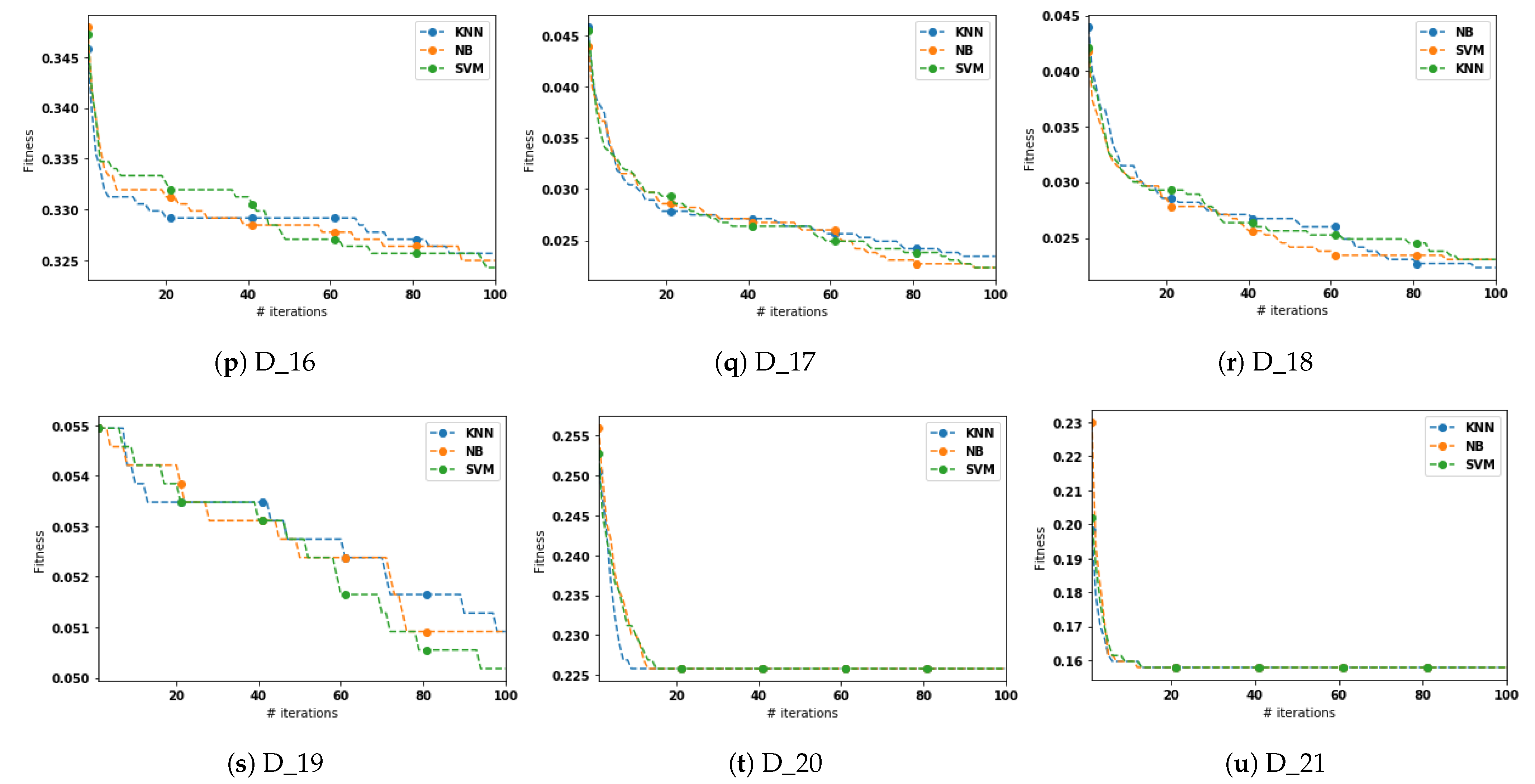
5.3. Results and Discussion

The methodology for applying training and testing in the experiments is based on a hold-out strategy in which each data set is split in a random way into 80% for training and 20% for testing. The experiments were repeated 30 times to obtain significant results. All experiments were conducted using a personal computer with AMD Athlon Dual-Core QL-60 CPU at 1.90 GHz and 2 GB of memory. The EvoloPy-FS [51] was used to run the experiments. It is a framework in Python for applying binary swarm intelligence algorithms to solve FS problems. It is open-source and available at (www.evo-ml.com accessed on 28 May 2021). The population size and the maximum iterations were set to 10 and 100, respectively [52].

Figure 5a illustrates the average recall obtained from applying the classifiers NB, KNN, and SVM without FS, with BMFO-FS, and with IsBMFO-FS. As can be seen, there was a dynamic increase in the values of recall. The lower values from the three classifiers were achieved when the classifiers were applied to the datasets without implementing FS. There was an increase in the recall values of the three classifiers when BMFO-FS was implemented. The best recall results were achieved when the IsBMFO-FS was implemented. This can be explained by the FS process having an effective influence on the classifiers’ performance. Furthermore, the island-based affected the performance of the classifiers and enhanced the optimizer job in the feature search space. In three experiments, the SVM classifier achieved the best performance, followed by the NB classifier. The lowest recall results were obtained by the KNN classifier. This can be explained by the SVM having the capability to distinguish between classes more than the KNN and NB. Furthermore, the integration of the FS process and the island enhancement helped to increase its efficiency. Figure 5b and Figure 6 show the results of the precision and gmean. As can be seen, the precision and gmean were increased dramatically when FS and FS with the island enhancement were applied to the BMFO.

Figure 7a,b and Figure 8 show the recall, precision, and recall results obtained from applying IsBMFO-FS to all the datasets. It can be noticed that the SVM classifier achieved the best results on most of the datasets. On the other hand, lower results were achieved by the NB and KNN classifiers. It can be noticed that the performance results of the NB and KNN were similar.

Figure 9 shows the convergence behavior of the three classifiers KNN, NB, and SVM with the proposed IsBMFO. It can be seen that the convergence behavior of the classifier SVM was better than the NB and KNN on 71% of the datasets. This can be seen in the tails of the convergence curves that reached low values of fitness. This means that IsBMFO with the SVM classifier can reach the global best in the time the other classifiers fall in the local minima. In addition, the classifier NB achieved better convergence scales compared with KNN on fifteen datasets. The convergence scales of the three classifiers were similar on six datasets: mw1, pc2, pc3, ant-1.7, xalan-2.6, and xerces-1.4.

Table 3. p-values of the Wilcoxon test for the IsBMFO-SVM and other classifiers using fitness (p > 0.05 are underlined).

Datasets	IsBMFO-KNN	IsBMFO-NB
D_1	2.44 $\times {10}^{-5}$	1.56 $\times {10}^{-5}$
D_2	4.31 $\times {10}^{-5}$	2.24 $\times {10}^{-4}$
D_3	1.21 $\times {10}^{-1}$	1.37 $\times {10}^{-1}$
D_4	1.28 $\times {10}^{-4}$	1.61 $\times {10}^{-10}$
D_5	1.31 $\times {10}^{-4}$	1.81 $\times {10}^{-9}$
D_6	1.23 $\times {10}^{-10}$	1.62 $\times {10}^{-10}$
D_7	2.38 $\times {10}^{-13}$	1.30 $\times {10}^{-12}$
D_8	2.46 $\times {10}^{-10}$	2.23 $\times {10}^{-10}$
D_9	4.52 $\times {10}^{-6}$	5.14 $\times {10}^{-7}$
D_10	4.95 $\times {10}^{-11}$	2.25 $\times {10}^{-11}$
D_11	3.14 $\times {10}^{-11}$	3.56 $\times {10}^{-10}$
D_12	6.63 $\times {10}^{-4}$	9.22 $\times {10}^{-14}$
D_13	9.41 $\times {10}^{-13}$	5.56 $\times {10}^{-12}$
D_14	1.78 $\times {10}^{-1}$	1.12 $\times {10}^{-1}$
D_15	2.32 $\times {10}^{-1}$	2.35 $\times {10}^{-5}$
D_16	2.23 $\times {10}^{-11}$	3.25 $\times {10}^{-12}$
D_17	5.18 $\times {10}^{-12}$	2.12 $\times {10}^{-13}$
D_18	4.13 $\times {10}^{-7}$	3.82 $\times {10}^{-7}$
D_19	3.66 $\times {10}^{-9}$	8.4 $\times {10}^{-12}$
D_20	2.61 $\times {10}^{-6}$	3.13 $\times {10}^{-7}$
D_21	2.65 $\times {10}^{-11}$	2.14 $\times {10}^{-11}$

shows p-values of the Wilcoxon test based on fitness. This statistical test takes into consideration all runs to determine if the IsBMFO-SVM is meaningfully different from other methods. Table 3 shows the superiority of IsBMFO-SVM over IsBMFO-NB and IsBMFO-KNN.

5.4. Analytical Description of the Relevant Features

This section presents an analytical description of the most informative features. These features are obtained by the IsBMFO-SVM approach. Referring to

Table 4. Relevant features in software datasets.

Datasets	AF	SF	FFR%	RF
cm1	38	15	61%	F2, F3, F7, F9, F11, F14, F17, F19, F23, F25, F26, F32, F33, F36, F38
jm1	22	9	59%	F1, F2, F4, F6, F7, F11, F13, F16, F19
kc1	22	8	64%	F3, F7, F9, F10, F14, F15, F18, F21
kc3	40	16	60%	F2, F4, F7, F8, F9, F11, F17, F19, F23, F26, F28, F31, F33, F35, F39, F40
mc1	39	12	69%	F3, F7, F8, F12, F13, F15, F20, F24, F28, F29, F32, F38
mw1	38	13	66%	F1, F5, F9, F11, F14, F16, F19, F20, F22, F25, F27, F30, F31
pc1	38	10	74%	F1, F6, F13, F15, F17, F21, F24, F27, F29, F35
pc2	37	14	62%	F1, F3, F4, F8, F13, F14, F17, F25, F27, F29, F30, F34, F36, F37
pc3	38	11	71%	F2, F3, F6, F9, F17, F20, F22, F26, F31, F34, F37
pc4	38	11	71%	F1, F5, F8, F9, F14, F22, F23, F26, F31, F35, F38
pc5	39	12	69%	F2, F4, F8, F10, F12, F15, F19, F25, F29, F30, F32, F37
ant-1.7	21	7	67%	F1, F5, F7, F10, F16, F19, F21
camel-1.6	21	9	57%	F2, F5, F6, F9, F11, F12, F14, F17, F20
ivy-2.0	21	10	52%	F3, F7, F10, F11, F13, F15, F16, F19, F20, F21
jedit-4.3	21	11	48%	F1, F4, F5, F7, F9, F13, F14, F15, F18, F20, F21
log4j-1.2	21	8	62%	F6, F9, F10, F13, F15, F17, F20, F21
lucene-2.4	21	9	57%	F2, F4, F7, F10, F11, F15, F18, F19, F21
poi-3.0	21	11	48%	F2, F5, F7, F8, F9, F10, F11, F14, F17, F19, F21
tomcat-6	20	7	65%	F4, F5, F8, F11, F13, F19, F20
xalan-2.6	21	8	62%	F1, F3, F6, F10, F11, F12, F19, F20
xerces-1.4	21	10	52%	F1, F4, F6, F7, F8, F11, F14, F16, F20, F21

, it shows the # all features in each dataset (AF), the number of selected features (SF), the feature reduction ratio (FRR), and the selected relevant features (RF) in the dataset. For the FFR, it is calculated by Equation (12).

$$\mathrm{FFR}=\frac{\mathrm{AF}-\mathrm{SF}}{\mathrm{AF}}$$

(12)

As can be seen, the FFR ranged between 48% on poi-3.0 and jedit-4.3 datasets to 74% on pc1 dataset. The average FRR on all the datasets is 62%. This ratio indicates that the proposed IsBMFO-SVM can reduce the dimensionality of the datasets by more than half. This supports the proposed IsBMFO-SVM, which also outperformed other approaches in terms of recall, precision, gmean, and convergence scales.

6. Conclusions and Future Trends

This paper proposes the island model to enhance the BMFO for solving the FS problem in the domain of software defect prediction. The new variant is called (IsBMFO). The island model divides the population of moths into a set of islands and applies a migration process to share features between islands. This concept can improve the diversity of solutions and control the convergence of the algorithm. In IsMFO, different copies of MFO are applied separately on each island in an asynchronous way. Three measurements are used to evaluate the proposed approach, recall, precision, and G-mean, in addition to the convergence scales and statistical rank test. The experiments compared the average recall, precision, and gmean obtained from applying the classifiers NB, KNN, and SVM without FS, with BMFO-FS, and with IsBMFO-FS. There was a dynamic increase in the values of the evaluation measures. The lower values from the three classifiers were achieved when the classifiers were applied to the datasets without implementing FS. The best results were achieved when the IsBMFO-FS was implemented. In three experiments, the SVM classifier achieved the best performance, followed by the NB classifier. The lowest results were obtained by the KNN classifier. Furthermore, the convergence behavior of the classifier SVM was better than the NB and KNN on 71% of the datasets.

The best achieved results were obtained by the IsBMFO-SVM model. These results demonstrate that the proposed model can serve as an effective predictive model for the software defect problem.

For future works, we suggest applying the proposed model on other classification problems such as for medical diagnosis. Furthermore, the island-based enhancement can be investigated with other metaheuristic algorithms.

References

1. Levendel, Y. Reliability analysis of large software systems: Defect data modeling. IEEE Trans. Softw. Eng. 1990, 16, 141–152. [Google Scholar] [CrossRef]
2. Ehrlich, W.K.; Iannino, A.; Prasanna, B.; Stampfel, J.P.; Wu, J.R. How faults cause software failures: Implications for software reliability engineering. In Proceedings of the 1991 International Symposium on Software Reliability Engineering, Austin, TX, USA, 17–18 May 1991; IEEE Computer Society: Washington, DC, USA, 1991; pp. 233–234. [Google Scholar]
3. Laprie, J.C. Dependability of computer systems: Concepts, limits, improvements. In Proceedings of the IEEE Sixth International Symposium on Software Reliability Engineering (ISSRE’95), Toulouse, France, 24–27 October 1995; pp. 2–11. [Google Scholar]
4. Mandeville, W.A. Software costs of quality. IEEE J. Sel. Areas Commun. 1990, 8, 315–318. [Google Scholar] [CrossRef]
5. Singpurwalla, N.D. Determining an optimal time interval for testing and debugging software. IEEE Trans. Softw. Eng. 1991, 17, 313–319. [Google Scholar] [CrossRef]
6. Mens, T.; Tourwé, T. A survey of software refactoring. IEEE Trans. Softw. Eng. 2004, 30, 126–139. [Google Scholar] [CrossRef] [Green Version]
7. Alsawalqah, H.; Hijazi, N.; Eshtay, M.; Faris, H.; Radaideh, A.A.; Aljarah, I.; Alshamaileh, Y. Software defect prediction using heterogeneous ensemble classification based on segmented patterns. Appl. Sci. 2020, 10, 1745. [Google Scholar] [CrossRef] [Green Version]
8. Wahono, R.S. A systematic literature review of software defect prediction. J. Softw. Eng. 2015, 1, 1–16. [Google Scholar]
9. Li, Z.; Jing, X.; Zhu, X. Progress on approaches to software defect prediction. IET Softw. 2018, 12, 161–175. [Google Scholar] [CrossRef]
10. Son, L.H.; Pritam, N.; Khari, M.; Kumar, R.; Phuong, P.T.M.; Thong, P.H. Empirical study of software defect prediction: A systematic mapping. Symmetry 2019, 11, 212. [Google Scholar] [CrossRef] [Green Version]
11. Shen, Z.; Chen, S. A Survey of Automatic Software Vulnerability Detection, Program Repair, and Defect Prediction Techniques. Secur. Commun. Netw. 2020, 2020, 8858010. [Google Scholar] [CrossRef]
12. Li, N.; Shepperd, M.; Guo, Y. A systematic review of unsupervised learning techniques for software defect prediction. Inf. Softw. Technol. 2020, 122, 106287. [Google Scholar] [CrossRef] [Green Version]
13. Aljarah, I.; Mafarja, M.; Heidari, A.A.; Faris, H.; Mirjalili, S. Multi-verse optimizer: Theory, literature review, and application in data clustering. In Nature-Inspired Optimizers; Springer: Cham, Switzerland, 2020; pp. 123–141. [Google Scholar]
14. Mafarja, M.; Heidari, A.A.; Faris, H.; Mirjalili, S.; Aljarah, I. Dragonfly algorithm: Theory, literature review, and application in feature selection. In Nature-Inspired Optimizers; Springer: Cham, Switzerland, 2020; pp. 47–67. [Google Scholar]
15. Singh, P.D.; Chug, A. Software defect prediction analysis using machine learning algorithms. In Proceedings of the 2017 IEEE 7th International Conference on Cloud Computing, Data Science & Engineering-Confluence, Noida, India, 12–13 January 2017; pp. 775–781. [Google Scholar]
16. Khurma, R.A.; Aljarah, I.; Sharieh, A. Rank based moth flame optimisation for feature selection in the medical application. In Proceedings of the 2020 IEEE Congress on Evolutionary Computation (CEC), Glasgow, UK, 19–24 July 2020; pp. 1–8. [Google Scholar]
17. Khurma, R.A.; Aljarah, I.; Sharieh, A. An Efficient Moth Flame Optimization Algorithm using Chaotic Maps for Feature Selection in the Medical Applications. In Proceedings of the 9th International Conference on Pattern Recognition Applications and Methods (ICPRAM), Valletta, Malta, 22–24 February 2020; pp. 175–182. [Google Scholar]
18. Faris, H.; Aljarah, I.; Alqatawna, J. Optimizing feedforward neural networks using krill herd algorithm for e-mail spam detection. In Proceedings of the 2015 IEEE Jordan Conference on Applied Electrical Engineering and Computing Technologies (AEECT), Amman, Jordan, 3–5 November 2015; pp. 1–5. [Google Scholar]
19. Khurma, R.A.; Aljarah, I.; Sharieh, A. A Simultaneous Moth Flame Optimizer Feature Selection Approach Based on Levy Flight and Selection Operators for Medical Diagnosis. Arab. J. Sci. Eng. 2021, 1–26. [Google Scholar] [CrossRef]
20. Agarwal, V.; Bhanot, S. Firefly inspired feature selection for face recognition. In Proceedings of the 2015 IEEE Eighth International Conference on Contemporary Computing (IC3), Noida, India, 20–22 August 2015; pp. 257–262. [Google Scholar]
21. Jouhari, H.; Lei, D.; Al-qaness, M.A.A.; Abd Elaziz, M.; Damaševičius, R.; Korytkowski, M.; Ewees, A.A. Modified Harris Hawks optimizer for solving machine scheduling problems. Symmetry 2020, 12, 1460. [Google Scholar] [CrossRef]
22. Sahlol, A.T.; Elaziz, M.A.; Jamal, A.T.; Damaševičius, R.; Hassan, O.F. A novel method for detection of tuberculosis in chest radiographs using artificial ecosystem-based optimisation of deep neural network features. Symmetry 2020, 12, 1146. [Google Scholar] [CrossRef]
23. Makhadmeh, S.N.; Al-Betar, M.A.; Alyasseri, Z.A.A.; Abasi, A.K.; Khader, A.T.; Damaševičius, R.; Mohammed, M.A.; Abdulkareem, K.H. Smart home battery for the multi-objective power scheduling problem in a smart home using grey wolf optimizer. Electronics 2021, 10, 447. [Google Scholar] [CrossRef]
24. Anbu, M.; Mala, G.A. Feature selection using firefly algorithm in software defect prediction. Clust. Comput. 2019, 22, 10925–10934. [Google Scholar] [CrossRef]
25. Khurma, R.; Castillo, P.; Sharieh, A.; Aljarah, I. Feature Selection using Binary Moth Flame Optimization with Time Varying Flames Strategies. In Volume 1: ECTA, INSTICC, Proceedings of the 12th International Joint Conference on Computational Intelligence, Budapest, Hungary, 2–4 November 2020; SciTePress: Setúbal, Portugal, 2020; pp. 17–27. [Google Scholar] [CrossRef]
26. Hussien, A.G.; Amin, M.; Abd El Aziz, M. A comprehensive review of moth-flame optimisation: Variants, hybrids, and applications. J. Exp. Theor. Artif. Intell. 2020, 32, 705–725. [Google Scholar] [CrossRef]
27. Shehab, M.; Abualigah, L.; Al Hamad, H.; Alabool, H.; Alshinwan, M.; Khasawneh, A.M. Moth–flame optimization algorithm: Variants and applications. Neural Comput. Appl. 2020, 32, 9859–9884. [Google Scholar] [CrossRef]
28. Kaur, K.; Singh, U.; Salgotra, R. An enhanced moth flame optimization. Neural Comput. Appl. 2020, 32, 2315–2349. [Google Scholar] [CrossRef]
29. Khurmaa, R.A.; Aljarah, I.; Sharieh, A. An intelligent feature selection approach based on moth flame optimization for medical diagnosis. Neural Comput. Appl. 2021, 33, 7165–7204. [Google Scholar] [CrossRef]
30. Xu, Y.; Chen, H.; Luo, J.; Zhang, Q.; Jiao, S.; Zhang, X. Enhanced Moth-flame optimizer with mutation strategy for global optimization. Inf. Sci. 2019, 492, 181–203. [Google Scholar] [CrossRef]
31. Khan, M.A.; Sharif, M.; Akram, T.; Damaševičius, R.; Maskeliūnas, R. Skin lesion segmentation and multiclass classification using deep learning features and improved moth flame optimization. Diagnostics 2021, 11, 811. [Google Scholar] [CrossRef]
32. Al-Betar, M.A.; Awadallah, M.A. Island bat algorithm for optimization. Expert Syst. Appl. 2018, 107, 126–145. [Google Scholar] [CrossRef]
33. Al-Betar, M.A.; Awadallah, M.A.; Doush, I.A.; Hammouri, A.I.; Mafarja, M.; Alyasseri, Z.A.A. Island flower pollination algorithm for global optimization. J. Supercomput. 2019, 75, 5280–5323. [Google Scholar] [CrossRef]
34. Al-Betar, M.A.; Awadallah, M.A.; Khader, A.T.; Abdalkareem, Z.A. Island-based harmony search for optimization problems. Expert Syst. Appl. 2015, 42, 2026–2035. [Google Scholar] [CrossRef]
35. Awadallah, M.A.; Al-Betar, M.A.; Bolaji, A.L.; Doush, I.A.; Hammouri, A.I.; Mafarja, M. Island artificial bee colony for global optimization. Soft Comput. 2020, 24, 13461–13487. [Google Scholar] [CrossRef]
36. Gupta, A.; Suri, B.; Kumar, V.; Misra, S.; Blažauskas, T.; Damaševičius, R. Software code smell prediction model using Shannon, Rényi and Tsallis entropies. Entropy 2018, 20, 372. [Google Scholar] [CrossRef] [PubMed] [Green Version]
37. Kumari, M.; Misra, A.; Misra, S.; Sanz, L.F.; Damasevicius, R.; Singh, V.B. Quantitative quality evaluation of software products by considering summary and comments entropy of a reported bug. Entropy 2019, 21, 91. [Google Scholar] [CrossRef] [PubMed] [Green Version]
38. Naidu, M.S.; Geethanjali, N. Classification of defects in software using decision tree algorithm. Int. J. Eng. Sci. Technol. 2013, 5, 1332–1340. [Google Scholar]
39. Can, H.; Xing, J.; Zhu, R.; Li, J.; Yang, Q.; Xie, L. A new model for software defect prediction using particle swarm optimization and support vector machine. In Proceedings of the 2013 IEEE 25th Chinese Control and Decision Conference (CCDC), Guiyang, China, 25–27 May 2013; pp. 4106–4110. [Google Scholar]
40. Shuai, B.; Li, H.; Li, M.; Zhang, Q.; Tang, C. Software defect prediction using dynamic support vector machine. In Proceedings of the 2013 IEEE Ninth International Conference on Computational Intelligence and Security, Emeishan, China, 14–15 December 2013; pp. 260–263. [Google Scholar]
41. Agarwal, S.; Tomar, D. A feature selection based model for software defect prediction. Int. J. Adv. Sci. Technol. 2014, 65, 39–58. [Google Scholar] [CrossRef]
42. Abaei, G.; Selamat, A. A survey on software fault detection based on different prediction approaches. Viet. J. Comput. Sci. 2014, 1, 79–95. [Google Scholar] [CrossRef]
43. Malhotra, R.; Nishant, N.; Gurha, S.; Rathi, V. Application of Particle Swarm Optimization for Software Defect Prediction Using Object Oriented Metrics. In Proceedings of the 2021 IEEE 11th International Conference on Cloud Computing, Data Science & Engineering (Confluence), Noida, India, 28–29 January 2021; pp. 88–93. [Google Scholar]
44. Balogun, A.O.; Basri, S.; Mahamad, S.; Abdulkadir, S.J.; Capretz, L.F.; Imam, A.A.; Almomani, M.A.; Adeyemo, V.E.; Kumar, G. Empirical Analysis of Rank Aggregation-Based Multi-Filter Feature Selection Methods in Software Defect Prediction. Electronics 2021, 10, 179. [Google Scholar] [CrossRef]
45. Mirjalili, S. Moth-flame optimization algorithm: A novel nature-inspired heuristic paradigm. Knowl. Based Syst. 2015, 89, 228–249. [Google Scholar] [CrossRef]
46. Mirjalili, S.; Lewis, A. S-shaped versus V-shaped transfer functions for binary particle swarm optimization. Swarm Evol. Comput. 2013, 9, 1–14. [Google Scholar] [CrossRef]
47. Kennedy, J.; Eberhart, R.C. A discrete binary version of the particle swarm algorithm. In Proceedings of the 1997 IEEE International conference on Systems, Man, and Cybernetics. Computational Cybernetics and Simulation, Orlando, FL, USA, 12–15 October 1997; Volume 5, pp. 4104–4108. [Google Scholar]
48. Kushida, J.i.; Hara, A.; Takahama, T.; Kido, A. Island-based differential evolution with varying subpopulation size. In Proceedings of the 2013 IEEE 6th International Workshop on Computational Intelligence and Applications (IWCIA), Hiroshima, Japan, 13 July 2013; pp. 119–124. [Google Scholar]
49. Michel, R.; Middendorf, M. An island model based ant system with lookahead for the shortest supersequence problem. In Proceedings of the International Conference on Parallel Problem Solving from Nature, Amsterdam, The Netherlands, 27–30 September 1998; Springer: Berlin/Heidelberg, Germany, 1998; pp. 692–701. [Google Scholar]
50. Araujo, L.; Merelo, J.J. Diversity through multiculturality: Assessing migrant choice policies in an island model. IEEE Trans. Evol. Comput. 2010, 15, 456–469. [Google Scholar] [CrossRef]
51. Khurma, R.A.; Aljarah, I.; Sharieh, A.; Mirjalili, S. Evolopy-fs: An open-source nature-inspired optimization framework in python for feature selection. In Evolutionary Machine Learning Techniques; Springer: Singapore, 2020; pp. 131–173. [Google Scholar]
52. Khurma, R.A.; Sabri, K.E.; Castillo, P.A.; Aljarah, I. Salp Swarm Optimization Search Based Feature Selection for Enhanced Phishing Websites Detection. In Proceedings of the Applications of Evolutionary Computation: 24th International Conference, EvoApplications 2021, Held as Part of EvoStar 2021, Virtual Event, 7–9 April 2021; Springer Nature: Basingstoke, UK, 2021; Volume 12694, pp. 146–161. [Google Scholar]
Figure 1. The spiral path of moths around a candle.
Mathematics 09 01722 g001
Figure 2. Architecture of the proposed methodology.
Mathematics 09 01722 g002
Figure 3. The flowchart of the proposed IsBMFO algorithm.
Mathematics 09 01722 g003
Figure 4. An illustration of island-based model.
Mathematics 09 01722 g004
Figure 5. Results of applying classifiers without FS, with BMFO-FS, and with IsBMFO-FS on all datasets. Average recall (a) and average precision (b).
Mathematics 09 01722 g005
Figure 6. Average gmean results of applying classifiers without FS, with BMFO-FS, and with IsBMFO-FS on all datasets.
Mathematics 09 01722 g006
Figure 7. Results of applying classifiers with IsBMFO-FS on all datasets. Average recall (a) and Average precision (b).
Mathematics 09 01722 g007
Figure 8. Gmean results of applying classifiers with IsBMFO-FS on all datasets.
Mathematics 09 01722 g008
Figure 9. Convergence curves for IsBMFO with the three classifiers KNN, NB, and SVM.
Mathematics 09 01722 g009aMathematics 09 01722 g009b