Application of EM Algorithm to NHPP-Based Software Reliability Assessment with Generalized Failure Count Data

Abstract

Software reliability models (SRMs) are widely used for quantitative evaluation of software reliability by estimating model parameters from failure data observed in the testing phase. In particular, non-homogeneous Poisson process (NHPP)-based SRMs are the most popular because of their mathematical tractability. In this paper, we focus on the parameter estimation algorithm for NHPP-based SRMs and discuss the EM algorithm for generalized fault count data. The presented algorithm can be applied for failure time data, failure count data, and their mixture. The paper derives the EM-step formulas for basic 12 NHPP-based SRMs and demonstrate a numerical experiment to present the convergence property of our algorithms. The developed algorithms are suitable for an automatic tool for software reliability evaluation.

1. Introduction

Software reliability models (SRMs) are used to assess quantitative reliability and to control the quality of software products. Since Jelinski and Moranda [1], and Goel and Okumoto [2] presented SRMs based on stochastic processes, numerous SRMs have been proposed [3,4,5,6,7,8]. In particular, non-homogeneous Poisson process (NHPP)-based SRMs have become popular in representing the dynamics of failure occurrence processes in a variety of situations [9,10,11,12,13]. By using an NHPP-based SRM, we predict the future behavior of software failure, i.e, the number of failures experienced in future, and estimate the quantitative measure of software reliability.

The advantage of NHPP-based SRMs is simplifying the stochastic analysis. NHPPs are generally dominated by mean value functions. The mean value function indicates the expected number of failures experienced at arbitrary testing time. By choosing appropriate mean value functions, NHPP-based SRMs can fit any observed failure data. The NHPP-based SRMs and the mean value functions have a one-to-one correspondence.

The Goel–Okumoto model [2]; Goel model [2]; Musa–Okumoto model [14]; Ohba [15,16]; Yamada, Ohba, and Osaki model [17]; Zhao and Xie model [18] are early NHPP-based SRMs. They were constructed with the deterministic debugging scenarios of mean value functions. Pham [19] solved a generalized differential equation by which the mean value function in the NHPP-based SRM is governed and proposed a generalized SRM with many redundant parameters.

Apart from such a deterministic modeling framework, almost all NHPP-based SRMs can be characterized as Markov processes. Shantikumar [20] discussed a modeling framework to integrate time-homogeneous Markov processes and NHPPs by using a binomial-type stochastic point process. Langberg and Singpurwalla [21] presented a unified modeling framework for almost all NHPP-based SRMs. Chen and Singpurwalla [22] also discussed the framework with a self-exciting point process. Miller [23] introduced the concept of exponential order statistics and drastically extended Langberg and Singpurwalla’s idea. In fact, the realizations of NHPP-based SRM can be described by either the general order statistics or record value statistics of the underlying software fault data, where the fault-detection times are assumed to be independent and identically distributed (i.i.d.) random variables. Specifically, the general order statistics are based on the order of all the fault detection times, and the record value statistics focus on their maximum detection time.

In this paper, we focus on the parameter estimation problem of NHPP-based SRMs. In general, there are three steps to evaluating the software reliability with NHPP-based SRM. (i) Collect the failure data such as the number of detected bugs in the testing phase, (ii) estimate the model parameters of NHPP-based SRM to fit it to the collected data, and (iii) compute reliability measures from the NHPP-based SRM with the estimated parameters. Based on quantitative measures, we control the software development process. As a typical usage of NHPP-based SRM, we estimate the number of failures that will be experienced in the future and decide whether to continue testing the software or the software can be released. In other words, the parameter estimation of NHPP-based SRM is frequently executed in the software development phase. The computation cost of the estimation should be small in practice.

Therefore, many authors have concerns about the parameter estimation problem on NHPP-based SRMs. Nevertheless, in actual software reliability assessments, a few NHPP-based SRMs and familiar maximum likelihood (ML) estimation methods are still used conventionally. The main reason for this is that the practitioners wish to use intuitively simple statistical methods, which exclude empirically based tuning parameters for a few SRMs that have survived a long history of software reliability engineering. In fact, the Bayesian estimation methods are still minor in software engineering practice, although its theoretical benefit is recognized. On the other hand, ML estimation is based on the maximization of likelihood function with software failure data and possesses several rational properties such as asymptotic efficiency. Hossain and Dahiya [24] derived necessary and sufficient conditions that the maximum likelihood estimates (MLEs), which satisfy the non-linear likelihood equations, exist in Goel and Okumoto SRM [2]. Knafl and Morgan [25] presented a method to systematically solve the likelihood equations with two model parameters. Joe [26] also discussed the confidence interval of MLEs. Zhao and Xie [18] provided the MLEs for an extended Goel and Okumoto SRM. Jeske and Pham [27] discovered empirically that the MLEs in Goel and Okumoto SRM are not statistically consistent. It should be noted, however, that ML estimation is always possible for all NHPP-based SRMs. Even if the likelihood functions are strictly concave in model parameters, it is difficult to solve the likelihood equations analytically. For instance, in the cases where the likelihood functions are not concave and where there exists no solution for the likelihood equations inside the parameter space, the conventional methods to calculate the MLEs cannot be used. Usually, the Newton method and the Nelder–Mead method are used to solve the maximization problem in the existing literature. From the recent development of computational ability, it is becoming easier to handle a large-scale complex optimization problem.

On the other hand, it is known that the local convergence property of the Newton method is a weakness for practical application. The local convergence property means that the convergence radius of algorithm is limited, and thus, it may fail to obtain a result if we set unsuitable initial guesses. For example, when we develop the application to automatically obtain parameter estimates from given data, the local convergence property becomes troublesome when choosing the initial guesses. Therefore, the Newton method is not suitable for this purpose. Additionally, the Nelder–Mead method is one of the direct search methods. The convergence property of the Nelder–Mead method is improved from the Newton method. However, some design parameters should be provided appropriately for the Nelder–Mead method. Even if we use the Nelder–Mead algorithm, the convergence of algorithm is not always guaranteed for any given data.

From the early 2000s, our research group has developed an alternative parameter estimation algorithm based on the EM (expectation maximization) principle [28,29] and applied it to the software reliability assessment based on NHPP-based SRMs [30,31,32,33,34,35,36,37,38,39,40]. As another examples of EM algorithms in SRMs, Kimura and Yamada [41], Leadoux [42], and Okamura and Dohi [43] attempted to use EM algorithms to estimate the imperfect debugging model [44] and architecture-based SRMs [45,46]. Their models were based on the continuous-time Markov chain and are closely related to Markov-modulated Poisson processes and/or Markovian arrival processes. Additionally, Zeephongsekul et al. [47] and Nagaraju et al. [48] proposed ECM (expectaton conditional maximization) algorithms for NHPP-based SRMs to handle several specific models.

The EM algorithm is an algorithm that finds maximum likelihood estimates for a statistical model with incomplete data. The idea behind our EM algorithms is to find the incomplete data structure of NHPP-based SRMs. Concretely, in NHPP-based SRMs, we assume that the number of failures is finite due to a finite number of software bugs, but all of them cannot be observed, i.e., the number of reaming software failures can be regarded as missing data. From this insight, the EM algorithm for an individual NHPP-based SRM is developed. Although the convergence speed of EM algorithm is generally slower than other general-purpose numerical methods such as the Newton method, it has a global convergence property. This property allows us to reduce efforts in choosing good initial guesses for the model parameters and is suitable for automating the estimation procedure. In our past work [49], we summarized EM algorithms for 12 NHPP-based SRMs when the failure data were time data. The failure time data consisted of a set of exact failure times experienced. In practice, it is difficult to obtain exact failure times. Generally, we record failure count data consisting of the number of failures experienced for time intervals. For example, it is reasonable to record the number of failures per working day. From this reason, this paper presents the EM algorithms for 12 basic NHPP-based SRMs when the failure count data are given. In particular, we consider the generalized failure count data that involve both failure time and count data formats, and thus, the developed EM algorithms can be applied to either failure time data, failure count data, or their mixture.

We highlight our contributions here: (i) we derive the EM-step formula for NHPP-based SRMs with a finite number of failures under generalized fault count data, (ii) we derive concrete EM-step formulas for 12 basic NHPP-based SRMs, and (iii) we demonstrate the performance on the convergence property of the presented algorithms with real software failure data. To our best knowledge, this is the first paper that presents the EM algorithm for the generalized fault count data in 12 basic NHPP-based SRMs.

This paper is organized as follows. In Section 2, we introduce NHPP-based SRMs that are considered in this paper. In particular, NHPP-based SRMs are classified by failure time distribution and present the relationship between basic 12 NHPP-based SRMs and their failure time distributions. In Section 3, we derive the EM-step formulas for 12 basic NHPP-based SRMs. Section 4 is devoted to a numerical example to compare the convergence properties of EM algorithm, the Nelder–Mead method, and the quasi-Newton method. Finally, we conclude the paper with remarks in Section 5.

2. NHPP-Based SRMs

2.1. Model Description

Let $\{X(t),t\ge 0\}$ denote the number of software failures experienced before time t. We make the following model assumptions [21]:

• Assumption A: A software failure occurs at a random time. The probability distribution of all failure times are identical and mutually independent.
• Assumption B: The number of inherent software faults causing failures is finite.

Here, $F(t)$ and N are the cumulative distribution function of the failure time and the number of inherent faults. Then, the probability mass function of the cumulative number of failures experienced by time t is

$$P(X(t)=n)=\left(\genfrac{}{}{0pt}{}{N}{n}\right)F{(t)}^n\overline{F}{(t)}^{N-n},$$

(1)

where $\overline{F}(·)=1-F(·)$. This is often called the framework of generalized order statistics [21]. For instance, when the failure distribution is an exponential distribution, the corresponding SRM, the so-called exponential order statistics model, is the same as the Jelinski–Moranda SRM [1].

Most NHPP-based SRMs are advanced models of the generalized order statistics models. We make an additional model assumption [21]:

• Assumption C: The number of inherent faults is unknown, but prior information is given by a Poisson distribution.

When the expected number of inherent faults is $\omega$, the cumulative number of software failures at time t has the following probability mass function:

$$P(X(t)=n)=\frac{{\left(\omega F(t)\right)}^n}{n!}{e}^{-\omega F(t)}.$$

(2)

Equation (2) is equivalent to the probability mass function of NHPP with mean value function $\omega F(t)$. In this modeling framework, the failure time distribution $F(t)$ specifies an NHPP-based SRM.

Since the NHPP-based SRM is characterized by the failure time distribution, there have been a number of NHPP-based SRMs that change the failure time distribution. In this paper, we propose basic NHPP-based SRMs using well-known statistical distributions as the failure time distribution.

Table 1. Basic NHPP-based SRMs.

Model	Failure Time Distribution
exp	Exponential distribution [2]
gamma	Gamma distribution [17,18]
pareto	Pareto type-II distribution [50]
tnorm	Truncated normal distribution [34]
lnorm	Log-normal distribution [34]
tlogis	Truncated logistic distribution [15]
llogis	Log-logistic distribution [52]
txvmax	Truncated extreme-value distribution (max) [35]
lxvmax	Log-extreme-value distribution (max) [35]
txvmin	Truncated extreme-value distribution (min) [35]
lxvmin	Log-extreme-value distribution (min) [35,51]

shows 11 basic NHPP-based SRMs and their failure time distributions. In the table, most of the basic NHPP-based SRMs correspond to the existing traditional NHPP-based SRMs. ‘exp’ is the so-called Goel and Okumoto model [2], ‘gamma’ is a generalized delayed S-shaped model [17,18], ‘pareto‘ is a modified Duane model [50], ‘tlogis‘ is an inflection S-shaped model [15], and ‘lxvmin‘ is the Goel (Weibull) model [51].

2.2. Parameter Estimation

As mentioned before, the model parameters of NHPP-based SRMs should be estimated from software failure data to predict the future tendency of a software failure. The most commonly used technique for parameter estimation is maximum likelihood (ML) estimation. In the context of ML estimation, we found model parameters that maximize the log-likelihood function (LLF). Since the LLF depends on the failure data experienced, the ML estimation of NHPP-based SRMs has been discussed for two types of data: failure time data and count data. The failure time data is a set of exact times in which a software failure occurs in the testing phase. The count data, equivalently called grouped data, consists of the number of failures experienced for time intervals. The estimation problems for these two data structures have been discussed separately.

This paper deals with a generalized data structure to express both failure time and count data. Our data structure is $\mathcal{D}:=\{(t_1,x_1,u_i),\dots ,(t_k,x_k,u_k)\}$, where $x_i$ failures that occur at the ith time interval, $(x_{i-1},x_i)$. In addition, if $u_i=1$, an additional failure occurs at the end of the ith time interval, i.e, at time $x_i$. Otherwise, if $u_i=0$, no failure occurs at the instant. If $u_i=0$ for all time intervals, the data turns out the failure count data. If $x_i=0$ and $u_i=1$ for all i, $\mathcal{D}$ is the failure time data.

Based on the generalized data, the LLF for NHPP-based SRMs is written in the following form:

$$\begin{array}{cc}\hfill \mathrm{LLF}(\omega ,\mathit{\theta })& =\sum _{i=1}^k(x_i+u_i)log\omega +\sum _{i=1}^k{x}_{i}log\left\{F(t_i;\mathit{\theta })-F(t_{i-1};\mathit{\theta })\right\}\hfill \\ \hfill & +\sum _{i=1}{u}_{i}logf(t_i;\mathit{\theta })-log{x}_i!-\omega F(t_k;\mathit{\theta }).\hfill \end{array}$$

(3)

Then, the problem is to find the optimal $(\omega ,\mathit{\theta })$, so-called maximum likelihood estimates (MLEs), maximizing $\mathrm{LLF}(\omega ,\mathit{\theta })$. However, it is noted that we cannot derive the closed form solution of MLEs. That is, we need to utilize numerical optimization techniques such as the Newton method, quasi-Newton method, and Nelder–Mead method.

Although conventional methods such as the Newton method and the Nelder–Mead method may be occasionally useful in computing MLEs of the NHPP-based SRMs, it is worth noting that these aim to solve unconstrained optimization problems in ML estimation. However, in many cases, we have to cope with constrained optimization problems because almost all of the model parameters of NHPP-based SRMs are implicitly constrained, such as positive constraint.

3. EM Algorithms for NHPP-Based SRMs

This paper develops numerical procedures to compute MLEs for NHPP-based SRMs with generalized data. The proposed estimation algorithms are based on the EM principle. The EM algorithm is one of the statistical approaches to compute the MLEs for incomplete data and is numerically stable because of its global convergence property. Moreover, the proposed EM algorithms for NHPP-based SRMs are based on the closed forms of MLEs for an arbitrary fault-detection time distribution and are capable of solving constrained optimization problems. Although we have already developed EM algorithms for failure time data and failure count data for several basic NHPP-based SRMs, this paper revisits their EM algorithm when generalized data are given.

3.1. EM Algorithm

The EM algorithm is an iterative method for computing ML estimates with incomplete data [28,29]. Let $\mathcal{D}$ and $\mathcal{U}$ be observable and unobservable data vectors, respectively, and $\mathit{\theta }$ be a model parameter vector $\mathit{\theta }$ to be estimated from only the observable data. In the ML estimation, we find a parameter vector by maximizing the following log-likelihood function (LLF) $\mathcal{L}(\mathit{\theta };\mathcal{D})$:

$$\begin{array}{c}\hfill \mathcal{L}(\mathit{\theta };\mathcal{D})=logp(\mathcal{D};\mathit{\theta })=log\int p(\mathcal{D},\mathcal{U};\mathit{\theta })d\mathcal{U},\end{array}$$

(4)

where $p(·)$ is any probability density or mass function and thus $p(\mathcal{D},\mathcal{U};\mathit{\theta })$ denotes the likelihood function for complete data $(\mathcal{D},\mathcal{U})$.

Let $Q(\mathit{\theta }|{\mathit{\theta }}^{\prime })$ denote the conditional expected LLF with respect to the complete data vector $(\mathcal{D},\mathcal{U})$ using the posterior distribution for unobservable data vector with a given parameter vector ${\mathit{\theta }}^{\prime }$:

$$\begin{array}{cc}\hfill Q(\mathit{\theta }|{\mathit{\theta }}^{\prime })& =E[logp(\mathcal{D},\mathcal{U};\mathit{\theta })|\mathcal{D};{\mathit{\theta }}^{\prime }]\hfill \\ \hfill & =\int p(\mathcal{U}|\mathcal{D};{\mathit{\theta }}^{\prime })logp(\mathcal{D},\mathcal{U};\mathit{\theta })d\mathcal{U}.\hfill \end{array}$$

(5)

Then, the EM algorithm consists of an E-step and an M-step. The E-step computes the conditional expected LLF with respect to the complete data vector $(\mathcal{D},\mathcal{U})$ using the posterior distribution for unobservable data vector with provisional parameter vector ${\mathit{\theta }}^{\prime }$, i.e., $Q(\mathit{\theta }|{\mathit{\theta }}^{\prime })$. In the M-step, we find a new parameter vector ${\mathit{\theta }}^{″}$ that maximizes the expected LLF:

$$\begin{array}{c}\hfill {\mathit{\theta }}^{″}:=\underset{\mathit{\theta }}{\mathrm{argmax}}Q(\mathit{\theta }|{\mathit{\theta }}^{\prime }),\end{array}$$

(6)

and ${\mathit{\theta }}^{″}$ becomes a provisional parameter vector at the next E- and M-steps. These steps surely increase the marginal LLF. The E- and M-steps are repeatedly executed until the parameters converge.

3.2. EM Algorithm for NHPP-Based SRMs

Consider the complete data in NHPP-based SRMs, $T_1<T_2<\dots <T_N$, where $T_i$ is the ith failure time and N is the number of all the failures. It is worth noting that the number of all the failures in software is unobserved. Since N is the Poisson-distributed random variable and $T_i$ obeys $F(·;\mathit{\theta })$, the complete LLF is given by

$$\mathrm{LLF}(\omega ,\mathit{\theta })=Nlog\omega -\omega +\sum _{i=1}^{N}logf(T_i;\mathit{\theta }).$$

(7)

From the standard argument of MLEs, the MLEs of $\omega$ and $\mathit{\theta }$ can be derived as

$$\omega =N$$

(8)

and

$$\mathit{\theta }=\underset{\mathit{\theta }}{\mathrm{argmax}}\sum _{i=1}^{N}logf(T_i;\mathit{\theta })$$

(9)

respectively. These imply that the estimation problem of NHPP-based SRMs under complete data can be decomposed into separate problems for two distribution functions: Poisson distribution and the failure time distribution.

Since the number of failures and the exact failure time in intervals are unobserved, the generalized data $\mathcal{D}:=\{(t_1,x_1,u_1),\dots ,(t_k,x_k,u_k)\}$ are incomplete data. By applying the EM algorithm, we have the following EM-step formulas for NHPP-based SRMs with the generalized data:

$$\omega \leftarrow \mathrm{E}\left[N\right|\mathcal{D};{\omega }^{\prime },{\mathit{\theta }}^{\prime }]$$

(10)

and

$$\mathit{\theta }\leftarrow \underset{\mathit{\theta }}{\mathrm{argmax}}\mathrm{E}\left[\left.\sum _{i=1}^{N}logf(T_i;\mathit{\theta })\right|\mathcal{D};{\omega }^{\prime },{\mathit{\theta }}^{\prime }\right]$$

(11)

Additionally, we obtain the following formula to compute the expected values. For any measurable function $h(·)$, the expected value with the generalized data is expressed as

$$\begin{array}{cc}\hfill \mathrm{E}\left[\left.\sum _{i=1}^{N}h(T_i)\right|\mathcal{D};{\omega }^{\prime },{\mathit{\theta }}^{\prime }\right]& =\sum _{i=1}^n\left\{\frac{x_i{\int }_{t_{i-1}}^{t_i}h(z)f(z;{\mathit{\theta }}^{\prime })dz}{{\int }_{t_{i-1}}^{t_i}f(z;{\mathit{\theta }}^{\prime })dz}+u_{i}h(t_i)\right\}\hfill \\ \hfill & +{\omega }^{\prime }{\int }_{t_k}^{\infty }h(z)f(z;{\mathit{\theta }}^{\prime })dz,\hfill \end{array}$$

(12)

where $f(z;\mathit{\theta })$ is a probability density function (p.d.f.) of failure time provided that the parameter vector is $\mathit{\theta }$. The derivation of this formula is given in Appendix A.

exp: ‘exp’ is the model where the failure time distribution is an exponential distribution. This model is exactly the same as the Goel–Okumoto model [2]. Define the c.d.f. of failure time as

$$F(t;\beta )=1-exp(-\beta t),\beta >0.$$

(13)

Since the MLE of an ordinary exponential distribution is given by a closed from, the EM-step formulas for exp are directly derived from Equations (10) and (11);

$$\begin{array}{cc}\hfill \omega & \leftarrow \mathrm{E}\left[N\right|\mathcal{D};{\omega }^{\prime },{\beta }^{\prime }]\hfill \end{array}$$

(14)

$$\begin{array}{cc}\hfill \beta & \leftarrow \frac{\mathrm{E}\left[N\right|\mathcal{D};{\omega }^{\prime },{\beta }^{\prime }]}{\mathrm{E}\left[{\sum }_{i=1}^N{T}_i\right|\mathcal{D};{\omega }^{\prime },{\beta }^{\prime }]}.\hfill \end{array}$$

(15)

By applying the formula for the expected value, we have

$$\begin{array}{cc}\hfill \omega & \leftarrow \sum _{i=1}^k(x_i+u_i)+{\omega }^{\prime }exp(-{\beta }^{\prime }{t}_k)\hfill \end{array}$$

(16)

$$\begin{array}{cc}\hfill \beta & \leftarrow \frac{{\sum }_{i=1}^k(x_i+u_i)+{\omega }^{\prime }exp(-{\beta }^{\prime }{t}_k)}{{\sum }_{i=1}^k(x_i{\tau }_i+u_i{t}_i)+{\omega }^{\prime }(t_k+1/{\beta }^{\prime })exp(-{\beta }^{\prime }{t}_k)}\hfill \end{array}$$

(17)

where

$${\tau }_i=\frac{(t_{i-1}+1/{\beta }^{\prime })exp(-{\beta }^{\prime }{t}_{i-1})-(t_i+1/{\beta }^{\prime })exp(-{\beta }^{\prime }{t}_i)}{exp(-{\beta }^{\prime }{t}_{i-1})-exp(-{\beta }^{\prime }{t}_i)}.$$

(18)

gamma: The failure time distribution becomes the following gamma distribution:

$$F(t;\alpha ,\beta )={\int }_0^t\frac{{\beta }^{\alpha }{u}^{\alpha -1}exp(-\beta u)}{\Gamma (\alpha )}du,\alpha >0,\beta >0,$$

(19)

where $\alpha$ and $\beta$ are shape and scale parameters, respectively. When $\alpha =2$ is fixed, the model reduces the delayed S-shaped SRM [17].

Similar to exp, the EM-step formulas are given using Equations (10) and (11):

$$\begin{array}{cc}\hfill \omega & \leftarrow \mathrm{E}\left[N\right|\mathcal{D};{\omega }^{\prime },{\alpha }^{\prime },{\beta }^{\prime }]\hfill \end{array}$$

(20)

$$\begin{array}{cc}\hfill \alpha & \leftarrow \left\{\alpha \right|log\alpha -\Psi (\alpha )=log\left(\frac{\mathrm{E}\left[{\sum }_{i=1}^N{T}_i\right|\mathcal{D};{\omega }^{\prime },{\alpha }^{\prime },{\beta }^{\prime }]}{\mathrm{E}\left[N\right|\mathcal{D};{\omega }^{\prime },{\alpha }^{\prime },{\beta }^{\prime }]}\right)\hfill \\ \hfill & -\frac{\mathrm{E}[{\sum }_{i=1}^{N}log{T}_i|\mathcal{D};{\omega }^{\prime },{\alpha }^{\prime },{\beta }^{\prime }]}{\mathrm{E}\left[N\right|\mathcal{D};{\omega }^{\prime },{\alpha }^{\prime },{\beta }^{\prime }]}\}\hfill \end{array}$$

(21)

$$\begin{array}{cc}\hfill \beta & \leftarrow \frac{\alpha \mathrm{E}\left[N\right|\mathcal{D};{\omega }^{\prime },{\alpha }^{\prime },{\beta }^{\prime }]}{\mathrm{E}\left[{\sum }_{i=1}^N{T}_i\right|\mathcal{D};{\omega }^{\prime },{\alpha }^{\prime },{\beta }^{\prime }]},\hfill \end{array}$$

(22)

where $\psi (·)$ is the digamma function, i.e., $\psi (\alpha )=dlog\gamma (\alpha )/d\alpha$. Additionally, we use the updated $\alpha$ to compute $\beta$. Note that Equation (21) can easily be solved with the nonlinear equation solver such as a bisection method. In addition, $\mathrm{E}\left[N\right|\mathcal{D};{\omega }^{\prime },{\alpha }^{\prime },{\beta }^{\prime }]$ and $\mathrm{E}\left[{\sum }_{i=1}^N{T}_i\right|\mathcal{D};{\omega }^{\prime },{\alpha }^{\prime },{\beta }^{\prime }]$ are obtained as follows:

$$\begin{array}{cc}\hfill & \mathrm{E}\left[N\right|\mathcal{D};{\omega }^{\prime },{\alpha }^{\prime },{\beta }^{\prime }]=\sum _{i=1}^k(x_i+u_i)+{\omega }^{\prime }\overline{F}(t_k;{\alpha }^{\prime },{\beta }^{\prime })\hfill \end{array}$$

(23)

$$\begin{array}{cc}\hfill & \mathrm{E}\left.\left[\sum _{i=1}^N{T}_i\right|\mathcal{D};{\omega }^{\prime },{\alpha }^{\prime },{\beta }^{\prime }\right]=\sum _{i=1}^k(x_i{\tau }_i+u_i{t}_i)+{\omega }^{\prime }({\alpha }^{\prime }/{\beta }^{\prime })\overline{F}(t_k;{\alpha }^{\prime }+1,{\beta }^{\prime }),\hfill \end{array}$$

(24)

$$\begin{array}{cc}\hfill & {\tau }_i=\frac{{\alpha }^{\prime }}{{\beta }^{\prime }}\frac{\overline{F}(t_{i-1};{\alpha }^{\prime }+1,{\beta }^{\prime })-\overline{F}(t_i;{\alpha }^{\prime }+1,{\beta }^{\prime })}{\overline{F}(t_{i-1};{\alpha }^{\prime },{\beta }^{\prime })-\overline{F}(t_i;{\alpha }^{\prime },{\beta }^{\prime })},\hfill \end{array}$$

(25)

where $\overline{F}(t;\alpha ,\beta )$ is the complementary c.d.f. of gamma distribution with parameters $\alpha$ and $\beta$. On the other hand, we need the numerical integration to obtain $\mathrm{E}[{\sum }_{i=1}^{N}log{T}_i|\mathcal{D};{\omega }^{\prime },{\alpha }^{\prime },{\beta }^{\prime }]$. It should be noted that, if the shape parameter $\alpha$ is fixed, then the computation algorithm becomes simple because we ignore solving the nonlinear equation and computing the expected value $\mathrm{E}[{\sum }_{i=1}^{N}log{T}_i|\mathcal{D};{\omega }^{\prime },{\alpha }^{\prime },{\beta }^{\prime }]$.

pareto: ‘pareto’ is the SRM where the failure time distribution is the Pareto distribution of the second kind. The Pareto distribution of the second kind is called Lomax distribution:

$$F(t)=1-\frac{c^a}{{(x+c)}^a},a>0,c>0.$$

(26)

This model was proposed as the modified Duane model [50].

Since the Pareto distribution of the second kind is a mixture of exponential distribution, the EM algorithm for ‘pareto’ is constructed using this property. In general, the mixture distribution is defined as a superposition of original statistical distributions with mixture ratio. Let $G(\xi ;\mathit{\theta })$ be the c.d.f. of mixture ratio distribution for the parameter $\xi$. Then, the mixture distribution is given by

$$F_M(x;\mathit{\theta })=\int F(x;\xi )dG(\xi ;\mathit{\theta }).$$

(27)

The Pareto distribution of the second kind is a mixture of exponential distribution when the mixture ratio distribution is a gamma distribution. That is, the failure time distribution is written in the following form:

$$\begin{array}{c}\hfill F(t;a,c)={\int }_0^{\infty }\left\{1-exp(-\xi t)\right\}\frac{c^a{\xi }^{a-1}exp(-c\xi )}{\Gamma (a)}d\xi =1-\frac{c^a}{{(c+t)}^a}.\end{array}$$

(28)

For the EM algorithm of mixture-type SRMs, we also define the fault detection rate for each fault as a hidden variable.

Let $(T_1,{\Xi }_1),\dots ,(T_N,{\Xi }_N)$ be a set of failure time and its associated fault detection rate for all the failures. The complete LLF is given by

$$\begin{array}{cc}\hfill \mathrm{LLF}(\omega ,a,c)=& Nlog\omega -\omega +\sum _{i=1}^{N}log{\Xi }_i-\sum _{i=1}^N{\Xi }_i{T}_i\hfill \\ \hfill & +aNlogc+(a-1)\sum _{i=1}^{N}log{\Xi }_i-c\sum _{i=1}^N{\Xi }_i-Nlog\Gamma (a).\hfill \end{array}$$

(29)

Similar to gamma, we have the following EM-step formula from the MLEs of gamma distributions:

$$\begin{array}{cc}\hfill & \omega \leftarrow \mathrm{E}\left[N\right|\mathcal{D};{\omega }^{\prime },a^{\prime },c^{\prime }],\hfill \end{array}$$

(30)

$$\begin{array}{cc}\hfill & a\leftarrow \left\{a\left|loga-\psi (a)=log\left(\frac{\mathrm{E}\left[{\sum }_{i=1}^N{\Xi }_i\right|\mathcal{D};{\omega }^{\prime },a^{\prime },c^{\prime }]}{\mathrm{E}\left[N\right|\mathcal{D};{\omega }^{\prime },a^{\prime },c^{\prime }]}\right)-\frac{\mathrm{E}[{\sum }_{i=1}^{N}log{\Xi }_i|\mathcal{D};{\omega }^{\prime },a^{\prime },c^{\prime }]}{\mathrm{E}\left[N\right|\mathcal{D};{\omega }^{\prime },a^{\prime },c^{\prime }]}\right.\right\}\hfill \end{array}$$

(31)

$$\begin{array}{cc}\hfill & b\leftarrow \frac{a\mathrm{E}\left[N\right|\mathcal{D};{\omega }^{\prime },a^{\prime },c^{\prime }]}{\mathrm{E}\left[{\sum }_{i=1}^N{\Xi }_i\right|\mathcal{D};{\omega }^{\prime },a^{\prime },c^{\prime }]},\hfill \end{array}$$

(32)

On the other hand, the formula for the expected value is given by

$$\begin{array}{c}\hfill \mathrm{E}\left[\left.\sum _{i=1}^{N}h({\Xi }_i)\right|\mathcal{D};{\omega }^{\prime },{\mathit{\theta }}^{\prime }\right]=\sum _{i=1}^k\left\{\frac{x_i{\int }_{t_{i-1}}^{t_i}\tilde{h}(z;{\mathit{\theta }}^{\prime })dz}{{\int }_{t_{i-1}}^{t_i}\tilde{f}(z;{\mathit{\theta }}^{\prime })dz}+\frac{u_i\tilde{h}(t_i)}{\tilde{f}(t_i)}\right\}+{\omega }^{\prime }{\int }_{t_k}^{\infty }\tilde{h}(z;{\mathit{\theta }}^{\prime })dz,\end{array}$$

(33)

where $h(·)$ is an arbitrary measurable function and

$$\begin{array}{cc}\hfill & \tilde{h}(z;{\mathit{\theta }}^{\prime })=\int h(\xi )f(z;\xi )dG(\xi ;{\mathit{\theta }}^{\prime }),\hfill \end{array}$$

(34)

$$\begin{array}{cc}\hfill & \tilde{f}(z;{\mathit{\theta }}^{\prime })=\int f(z;\xi )dG(\xi ;{\mathit{\theta }}^{\prime }).\hfill \end{array}$$

(35)

tnorm, lnorm: ‘tnorm’ and ‘lnorm’ are SRMs whose failure time distributions are truncated and log normal distributions, respectively. The failure time distributions for tnorm and lnorm are

$$\begin{array}{cc}\hfill & \mathrm{tnorm}:F(t)=\Phi \left(\frac{t-\mu }{\sigma }\right)/\left\{1-\Phi (-\mu /\sigma )\right\},\hfill \end{array}$$

(36)

$$\begin{array}{cc}\hfill & \mathrm{lnorm}:F(t)=\Phi \left(\frac{logt-\mu }{\sigma }\right),\hfill \end{array}$$

(37)

where $\Phi (·)$ is the c.d.f. of the standard normal distribution. Since the EM algorithms for both models with failure time and count data were introduced in detail in the literature [34], this paper provides the EM-step formulas with the generalized data.

• EM-step formula for tnorm:

  $$\begin{array}{cc}\hfill & \tilde{\omega }\leftarrow N,\mu \leftarrow T^{(1)}/N,\sigma \leftarrow \sqrt{T^{(2)}/N-{(T^{(1)}/N)}^2}\hfill \end{array}$$

  (38)

  where

  $$\begin{array}{cc}\hfill & N=\sum _{i=1}^k(x_i+u_i)+\tilde{\omega }\{\Phi (z_0)+\overline{\Phi }(z_k)\},\hfill \end{array}$$

  (39)

  $$\begin{array}{cc}\hfill & T^{(1)}=\sum _{i=1}^k(x_i{\tau }_i^{(1)}+u_i{t}_i)+\tilde{\omega }\{{\Phi }^{(1)}(z_0)+{\overline{\Phi }}^{(1)}(z_k)\}\hfill \end{array}$$

  (40)

  $$\begin{array}{cc}\hfill & T^{(2)}=\sum _{i=1}^k(x_i{\tau }_i^{(2)}+u_i{t}_i^2)+\tilde{\omega }\{{\Phi }^{(2)}(z_0)+{\overline{\Phi }}^{(2)}(z_k)\},\hfill \end{array}$$

  (41)

  $$\begin{array}{cc}\hfill & z_0=-\mu /\sigma ,z_i=(t_i-\mu )/\sigma ,\hfill \end{array}$$

  (42)

  $$\begin{array}{cc}\hfill & {\tau }_i^{(u)}=\frac{{\overline{\Phi }}^{(u)}(z_{i-1})-{\overline{\Phi }}^{(u)}(z_i)}{\overline{\Phi }(z_{i-1})-\overline{\Phi }(z_i)},\hfill \end{array}$$

  (43)
• EM-step formula for lnorm:

  $$\begin{array}{cc}\hfill & \omega \leftarrow N,\mu \leftarrow T^{(1)}/N,\sigma \leftarrow \sqrt{T^{(2)}/N-{(T^{(1)}/N)}^2}\hfill \end{array}$$

  (44)

  where

  $$\begin{array}{cc}\hfill & N=\sum _{i=1}^k(x_i+u_i)+{\omega }^{\prime }\overline{\Phi }(z_k),\hfill \end{array}$$

  (45)

  $$\begin{array}{cc}\hfill & T^{(1)}=\sum _{i=1}^k(x_i{\tau }_i^{(1)}+u_{i}log{t}_i)+\omega {\overline{\Phi }}^{(1)}(z_k),\hfill \end{array}$$

  (46)

  $$\begin{array}{cc}\hfill & T^{(2)}=\sum _{i=1}^k(x_i{\tau }_i^{(2)}+u_i{(log{t}_i)}^2)+\omega {\overline{\Phi }}^{(2)}(z_k),\hfill \end{array}$$

  (47)

  $$\begin{array}{cc}\hfill & z_0\to -\infty ,z_i=(log{t}_i-\mu )/\sigma ,\hfill \end{array}$$

  (48)

  $$\begin{array}{cc}\hfill & {\tau }_i^{(u)}=\frac{{\overline{\Phi }}^{(u)}(z_{i-1})-{\overline{\Phi }}^{(u)}(z_i)}{\overline{\Phi }(z_{i-1})-\overline{\Phi }(z_i)}.\hfill \end{array}$$

  (49)

In the above formulas, $\overline{\Phi }(z)$ is the complementary c.d.f. of the standard normal distribution, and ${\overline{\Phi }}^{(1)}(z)$ and ${\overline{\Phi }}^{(2)}(z)$ are expressed with the p.d.f. of the standard normal distribution $\varphi (z)$:

$$\begin{array}{cc}\hfill & {\overline{\Phi }}^{(1)}(z)=\sigma \varphi (z)+\mu \overline{\Phi }(z),\hfill \end{array}$$

(50)

$$\begin{array}{cc}\hfill & {\overline{\Phi }}^{(2)}(z)=({\sigma }^{2}z+2\mu \sigma )\varphi (z)+({\sigma }^2+{\mu }^2)\overline{\Phi }(z).\hfill \end{array}$$

(51)

In addition, after the convergence, we take $\omega =\tilde{\omega }\overline{\Phi }(z_0)$ to obtain the ML estimate for $\omega$ in the case of tnorm.

tlogis, llogis tlogis and llogis are the SRMs with truncated and log logistic distributions, respectively. In particular, ‘tlogis‘ is equivalent to the inflection S-shaped model [15]. The failure time distribution of tlogis is given by

$$F(t)=\Psi \left(\frac{t-\mu }{\psi }\right)/\left\{1-\Psi (-\mu /\psi )\right\},$$

(52)

where $\Psi (·)$ is the c.d.f. of standard logistic distribution

$$\Psi (t)=\frac{1}{1+exp(-t)}.$$

(53)

By taking into account the exponential of logistic distribution, we have the following failure time distribution of llogis:

$$F(t)=\Psi \left(\frac{logt-\mu }{\psi }\right).$$

(54)

Since logistic distribution does not belongs to the exponential family of distributions, neither expectation nor maximization can be expressed as simple formulas. To construct the algorithm, we consider only one assumption; the number of all failures is not observed. Then, the EM-step formulas become

• The EM-step formula for tnorm

  $$\begin{array}{cc}\hfill & \tilde{\omega }\leftarrow \sum _{i=1}^k(x_i+u_i)+{\tilde{\omega }}^{\prime }F(0;{\mathit{\theta }}^{\prime })+{\tilde{\omega }}^{\prime }\overline{F}(t_k;{\mathit{\theta }}^{\prime })\hfill \end{array}$$

  (55)

  $$\begin{array}{cc}\hfill & \mathit{\theta }\leftarrow \underset{\mathit{\theta }}{\mathrm{argmax}}\{\sum _{i=1}^k\left(x_{i}log(F(t_i;\mathit{\theta })-F(t_{i-1};\mathit{\theta }))-x_{i}log{x}_i!+u_{i}logf(t_i;\mathit{\theta })\right)\hfill \\ \hfill & +({\tilde{\omega }}^{\prime }F(0;{\mathit{\theta }}^{\prime }))log(F(0;\mathit{\theta }))+({\tilde{\omega }}^{\prime }\overline{F}(t_k;{\mathit{\theta }}^{\prime }))log(\overline{F}(t_k;\mathit{\theta }))\}.\hfill \end{array}$$

  (56)
• The EM-step formula for lnorm

  $$\begin{array}{cc}\hfill & \omega \leftarrow \sum _{i=1}^k(x_i+u_i)+{\omega }^{\prime }\overline{F}(t_k;{\mathit{\theta }}^{\prime })\hfill \end{array}$$

  (57)

  $$\begin{array}{cc}\hfill & \mathit{\theta }\leftarrow \underset{\mathit{\theta }}{\mathrm{argmax}}\{\sum _{i=1}^k\left(x_{i}log(F(t_i;\mathit{\theta })-F(t_{i-1};\mathit{\theta }))-x_{i}log{x}_i!+u_{i}logf(t_i;\mathit{\theta })\right)\hfill \\ \hfill & +({\omega }^{\prime }\overline{F}(t_k;{\mathit{\theta }}^{\prime }))log(\overline{F}(t_k;\mathit{\theta }))\}.\hfill \end{array}$$

  (58)

The second equations in both formulas indicate that $\mathit{\theta }$ is updated by the MLEs when the number of all the failures is given by ${\tilde{\omega }}^{\prime }$ and ${\omega }^{\prime }$. These algorithm are also stable if there exists a unique solution maximizing the right-hand side of the second term. Note that, after the convergence, the model parameter $\omega$ in tlogis can be obtained as $\omega =\tilde{\omega }\overline{F}(0;\mathit{\theta })$.

txvmax, lxvmax, txvmin, lxvmin Suppose that the failure time caused by each failure follows an extreme value type I distribution. The extreme value type I distribution is called Gumbel distribution, and its definition is based on the limitation of the maximum value of random variables. Here, the c.d.f. of a standard Gumbel distribution is defined as

$$\Theta (t)=exp\{-exp(-t)\}.$$

(59)

Similar to tnorm, lnorm, tlogis, and llogis, we consider the truncation and logarithm of the extreme value distribution. In addition, since the extreme value distribution is not symmetric, we also consider the case of negative samples, i.e., the minimum value of random variables.

The failure time distributions of txvmax and lxvmax are, respectively,

$$\begin{array}{cc}\hfill & F(t)=\Theta \left(\frac{t-\mu }{\mathit{\theta }}\right)/\left\{1-\Theta (-\mu /\mathit{\theta })\right\},\hfill \end{array}$$

(60)

$$\begin{array}{cc}\hfill & F(t)=\Theta \left(\frac{logt-\mu }{\mathit{\theta }}\right).\hfill \end{array}$$

(61)

Similarly, the failure time distributions of txvmin and lxvmin are given by

$$\begin{array}{cc}\hfill & F(t)=\overline{\Theta }\left(\frac{t+\mu }{\mathit{\theta }}\right)/\left\{1-\overline{\Theta }(\mu /\mathit{\theta })\right\},\hfill \end{array}$$

(62)

$$\begin{array}{cc}\hfill & F(t)=\overline{\Theta }\left(\frac{logt+\mu }{\mathit{\theta }}\right),\hfill \end{array}$$

(63)

where $\overline{\Theta }(t)=1-\Theta (-t)$ corresponds to the c.d.f. of a standard extreme value type I distribution of the minimum. From Equation (63), we find that lxvmin is equivalent to the Weibull distribution.

Since the extreme value distribution is not an exponential family, we consider only one assumption; the number of all the failures is not observed. Then, the EM-step formulas are given by

• The EM-step formula for txvmax and txvmin

  $$\begin{array}{cc}\hfill & \tilde{\omega }\leftarrow \sum _{i=1}^k(x_i+u_i)+{\tilde{\omega }}^{\prime }F(0;{\mathit{\theta }}^{\prime })+{\tilde{\omega }}^{\prime }\overline{F}(t_k;{\mathit{\theta }}^{\prime })\hfill \end{array}$$

  (64)

  $$\begin{array}{cc}\hfill & \mathit{\theta }\leftarrow \underset{\mathit{\theta }}{\mathrm{argmax}}\{\sum _{i=1}^k\left(x_{i}log(F(t_i;\mathit{\theta })-F(t_{i-1};\mathit{\theta }))-x_{i}log{x}_i!+u_{i}logf(t_i;\mathit{\theta })\right)\hfill \\ \hfill & +({\tilde{\omega }}^{\prime }F(0;{\mathit{\theta }}^{\prime }))log(F(0;\mathit{\theta }))+({\tilde{\omega }}^{\prime }\overline{F}(t_k;{\mathit{\theta }}^{\prime }))log(\overline{F}(t_k;\mathit{\theta }))\}.\hfill \end{array}$$

  (65)
• The EM-step formula for lxvmax and lxvmin

  $$\begin{array}{cc}\hfill & \omega \leftarrow \sum _{i=1}^k(x_i+u_i)+{\omega }^{\prime }\overline{F}(t_k;{\mathit{\theta }}^{\prime })\hfill \end{array}$$

  (66)

  $$\begin{array}{cc}\hfill & \mathit{\theta }\leftarrow \underset{\mathit{\theta }}{\mathrm{argmax}}\{\sum _{i=1}^k\left(x_{i}log(F(t_i;\mathit{\theta })-F(t_{i-1};\mathit{\theta }))-x_{i}log{x}_i!+u_{i}logf(t_i;\mathit{\theta })\right)\hfill \\ \hfill & +({\omega }^{\prime }\overline{F}(t_k;{\mathit{\theta }}^{\prime }))log(\overline{F}(t_k;\mathit{\theta }))\}.\hfill \end{array}$$

  (67)

4. Numerical Example

We investigated the numerical characteristics of the presented EM algorithms. Here, we compare the convergence property with the Nelder–Mead method and the quasi-Newton method (BFGS method). First, we check the trace of model parameters until they converge to MLE for the proposed method (EM algorithm), the Nelder–Mead method, and the BFGS method. In this experiment, we used the fault count data, which were collected from real software projects [53]. The statistics of fault count data are given as follow.

• Data label: SS1A
• Working days: 151
• The number of failures: 112
• LOC: Hundreds of thousands
• Software type: Operations

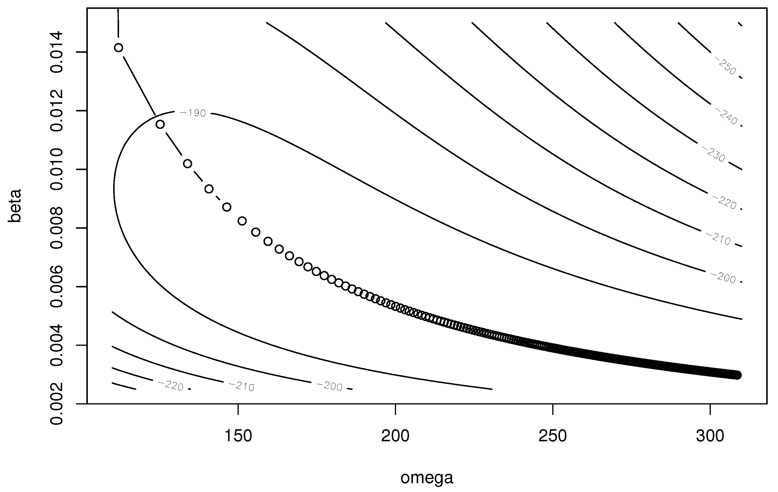
For the above failure count data, we estimated the parameters of ‘exp’. The MLEs of exp are $\widehat{\omega }=354.75$ and $\widehat{\beta }=0.00251$, and the maximum LLF is $\mathrm{LLF}(\widehat{\omega },\widehat{\beta })=-180.79$.

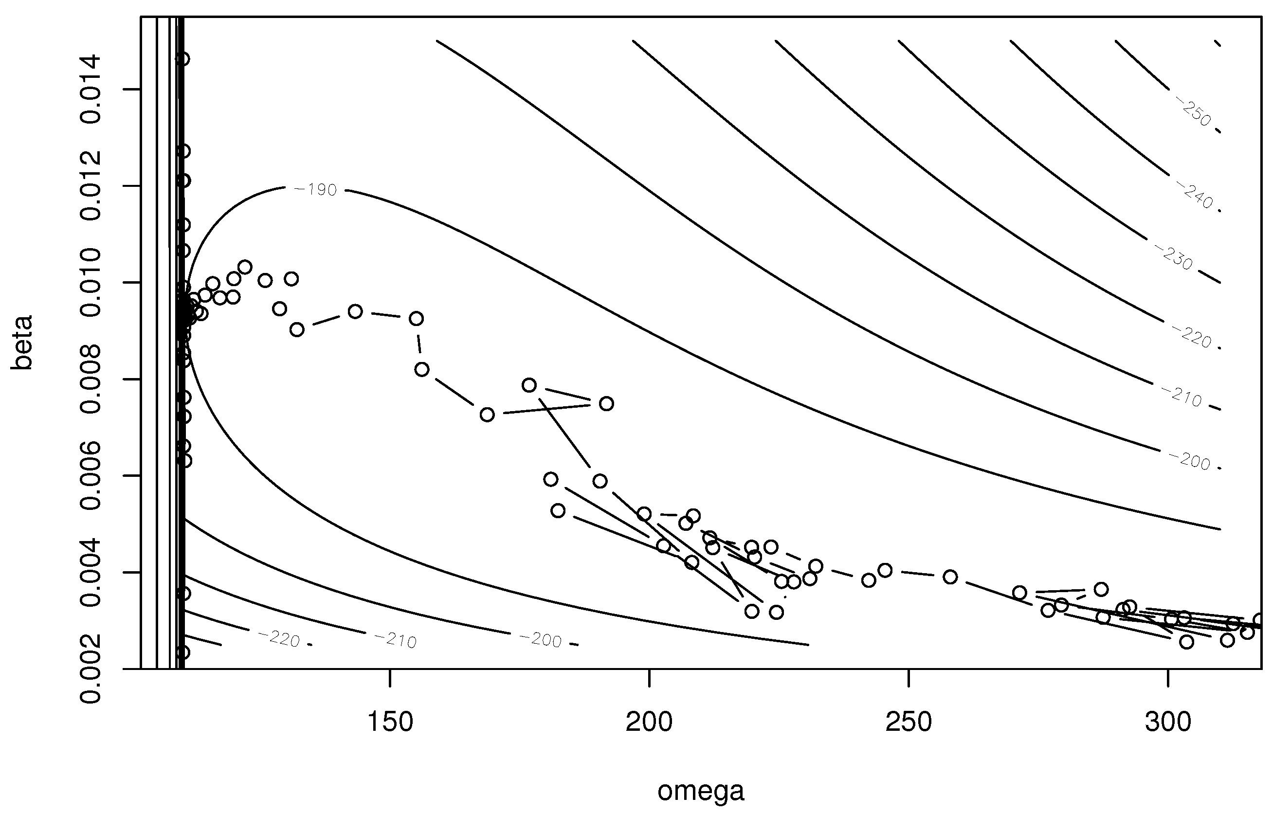
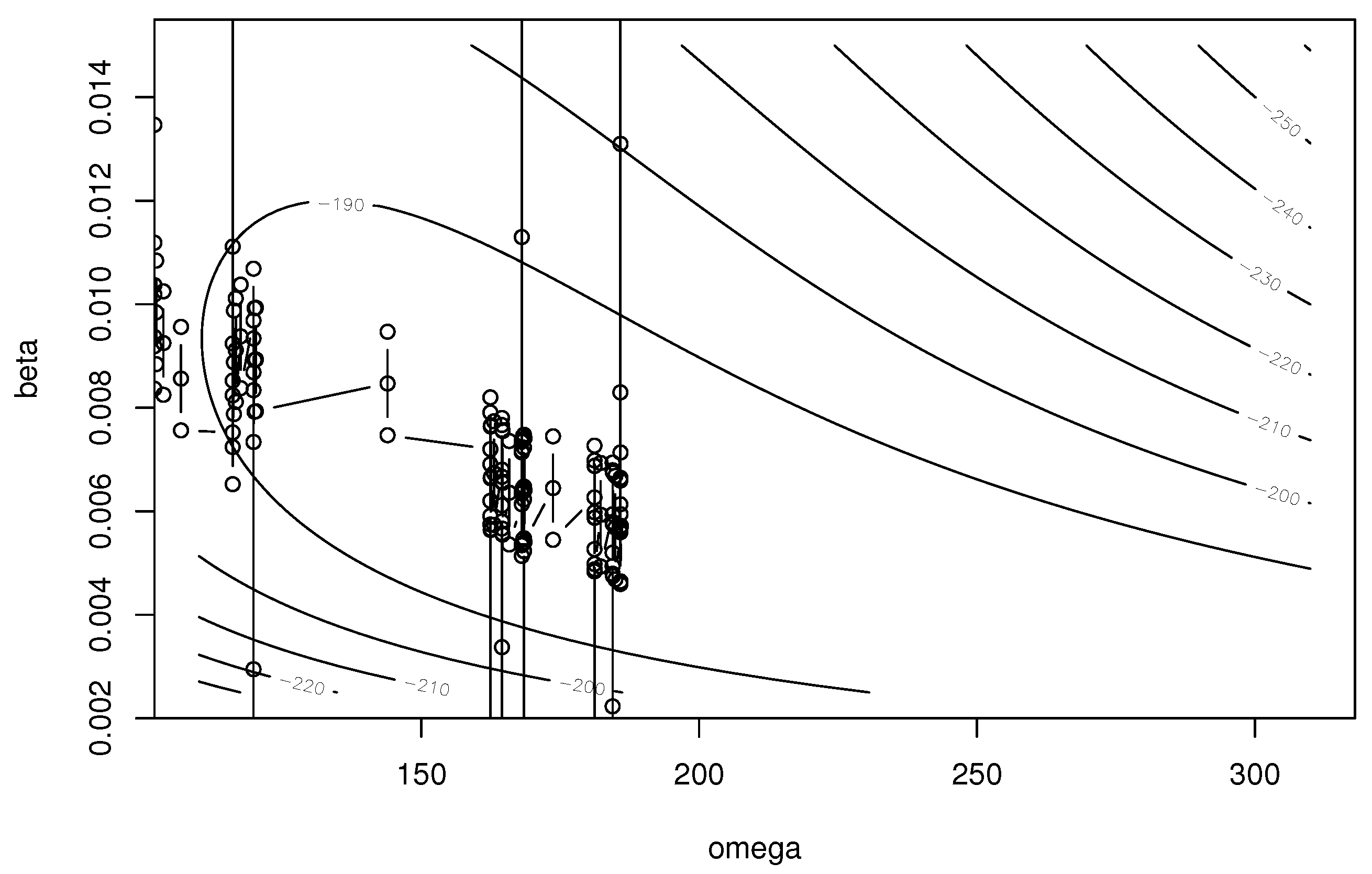
Figure 1, Figure 2 and Figure 3 show the trace of model parameters for EM algorithm, the Nelder–Mead method, and the BFGS method when the initial guesses are $\omega =100$ and $\beta =0.1$. We use the ‘optim’ function in R for the Nelder–Mead and BFGS methods. From these figures, we find that the EM algorithm stably updates the model parameters and converges to close parameters to the MLEs. However, the convergence speed is not fast, since the update becomes smaller as the parameters are close to the MLEs. The Nelder–Mead method provides the MLEs, but the trace of the algorithm is not stable. In particular, this algorithm sometimes takes invalid values that violate the parameter constraints, i.e., $\omega <0$ or $\beta <0$, while searching for the parameters. Figure 3 depicts the trace of parameters for the BFGS method. The convergence property is the worst among the three methods. Additionally, the algorithm fails to obtain the MLE.

Next, we present the convergence properties for the proposed EM algorithm, the Nelder–Mead method, and the BFGS method quantitatively. Here, we use two additional fault count data that were collected from real software projects [53] as well as SS1A.

• Data label: SS1B
• Working days: 663
• The number of failures: 375
• LOC: Hundreds of thousands
• Software type: Operations

• Data label: SS1C
• Working days: 472
• The number of failures: 277
• LOC: Hundreds of thousands
• Software type: Operations

For three data sets—SS1A, SS1B, and SS1C—we applied the proposed EM algorithm, the Nelder–Mead method, and the BFGS method for 12 basic NHPP-based SRMs with 100 different initial parameters. In the experiment, the initial parameters were selected by random numbers.

Table 2. The number of converged estimations (SS1A).

Model	EM	Nelder-Mead	BFGS
exp	100	19	19
gamma	100	34	34
pareto	100	57	57
tnorm	100	88	88
lnorm	100	98	98
tlogis	100	100	100
llogis	100	100	100
txvmax	100	100	100
lxvmax	99	99	99
txvmin	64	65	65
lxvmin	92	92	92

,

Table 3. The number of converged estimations (SS1B).

Model	EM	Nelder-Mead	BFGS
exp	100	7	7
gamma	100	7	6
pareto	100	18	18
tnorm	100	98	98
lnorm	87	87	87
tlogis	100	100	100
llogis	87	87	87
txvmax	99	99	99
lxvmax	0	0	0
txvmin	89	89	89
lxvmin	100	41	41

and

Table 4. The number of converged estimations (SS1C).

Model	EM	Nelder-Mead	BFGS
exp	100	9	8
gamma	100	13	12
pareto	100	47	47
tnorm	100	98	98
lnorm	96	97	97
tlogis	100	100	100
llogis	96	96	96
txvmax	99	99	99
lxvmax	0	0	0
txvmin	89	89	89
lxvmin	100	43	43

present the number of converged estimations, i.e., the number of times that the model parameters are successfully estimated for each NHPP-based SRMs and methods. If this value is 100, the method succeeded in obtaining the MLE for all of the initial parameters. On the other hand, if this value is 0, the estimation method fails to obtain the MLE for all of the initial parameters due to numerical computation errors such as overflow and underflow.

From these results, we find that the convergence rates of the proposed EM algorithms are 100% in the cases of exp, gamma, pareto, tnorm, and tlogis. Since the number of converged estimations of the Nelder–Mead is almost the same as that of BFGS for all cases, the convergence properties of their methods are the same if we use the ‘optim’ function in R. Additionally, since lxvmax did not fit SS1B and SS1C, all of the estimation methods failed to obtain the MLE. Furthermore, it was found that the numbers of converged estimates in the Nelder–Mead and BFGS methods are worse than that of the EM algorithm, specifically in the cases of exp, gamma, and pareto. Additionally, in the cases of tnorm and lnorm, the convergence property of EM is slightly superior to the other two methods. In exp, gamma, pareto, tnorm, and lnorm, the failure time distributions belong to the exponential family, and thus, their EM-step formulas do not include the numerical optimization step. That is, these EM-step formulas are ‘pure’ EM-step formulas. Therefore, the convergence properties outperform those of the Nelder–Mead and BFGS methods. On the other hand, in the cases of tlogis, llogis, txvmax, lxvmax, txvmin, and lvxmin, the failure time distributions are not in the exponential family, and we should use the numerical optimization step in their EM-step formulas. This is the reason why the convergence property of the presented EM algorithm is same as that in the Nelder–Mead and BFGS methods.

5. Conclusions

This paper derived EM-step formulas for 12 basic NHPP-based SRMs when the generalized failure count data are given. Since the generalized fault count data involve both time and count data formats, the presented EM algorithms can be applied to failure data experienced in practice. In addition, the convergence property of EM algorithm is better than or equivalent to other ordinary methods such as the Nelder–Mead and BFGS methods for practical software fault data. Thus, the presented algorithms are suitable for implementation in the automatic tool for software reliability evaluation. In fact, our research group has developed an AddIn of Microsoft Excel to estimate software reliability [54].

In the future, we will develop a reliability assessment tool by integrating a software repository such as GitHub, a bug tracking system, and a continuous integration system, and the tool will continuously monitor the reliability of software.

References

- Jelinski, Z.; Moranda, P.B. Software Reliability Research. In Statistical Computer Performance Evaluation; Freiberger, W., Ed.; Academic Press: New York, NY, USA, 1972; pp. 465–484. [Google Scholar]
- Goel, A.L.; Okumoto, K. Time-Dependent Error-Detection Rate Model for Software Reliability and Other Performance Measures. IEEE Trans. Reliab. 1979, R-28, 206–211. [Google Scholar] [CrossRef]
- Lyu, M.R. (Ed.) Handbook of Software Reliability Engineering; McGraw-Hill: New York, NY, USA, 1996. [Google Scholar]
- Musa, J.D.; Iannino, A.; Okumoto, K. Software Reliability, Measurement, Prediction, Application; McGraw-Hill: New York, NY, USA, 1987. [Google Scholar]
- Pham, H. Software Reliability; Springer: Singapore, 2000. [Google Scholar]
- Xie, M. Software Reliability Modelling; World Scientific: Singapore, 1991. [Google Scholar]
- Rook, P. (Ed.) Software Reliability Handbook; Elsevier Science: London, UK, 1990. [Google Scholar]
- Singpurwalla, N.D.; Wilson, S.P. Statistical Methods in Software Engineering; Springer: New York, NY, USA, 1997. [Google Scholar]
- Li, Q.; Pham, H. A Generalized Software Reliability Growth Model With Consideration of the Uncertainty of Operating Environments. IEEE Access 2019, 7, 84253–84267. [Google Scholar] [CrossRef]
- Li, Q.; Pham, H. NHPP software reliability model considering the uncertainty of operating environments with imperfect debugging and testing coverage. Appl. Math. Model. 2017, 51, 68–85. [Google Scholar] [CrossRef]
- He, Y. NHPP software reliability growth model incorporating fault detection and debugging. In Proceedings of the 2013 IEEE 4th International Conference on Software Engineering and Service Science, Beijing, China, 23–25 May 2013; pp. 225–228. [Google Scholar]
- Song, K.Y.; Chang, I.H.; Pham, H. NHPP Software Reliability Model with Inflection Factor of the Fault Detection Rate Considering the Uncertainty of Software Operating Environments and Predictive Analysis. Symmetry 2019, 11, 521. [Google Scholar] [CrossRef] [Green Version]
- Sun, H.; Zhang, L.; Wu, J.; Wu, J.; Yang, H. A New Method of Model Combination Based on the NHPP Software Reliability Models. In ICMSS 2018: Proceedings of the 2018 2nd International Conference on Management Engineering, Software Engineering and Service Sciences; ACM: New York, NY, USA, 2018; pp. 153–158. [Google Scholar] [CrossRef]
- Musa, J.D.; Okumoto, K. A Logarithmic Poisson Execution Time Model for Software Reliability Measurement. In Proceedings of the 7th International Conference Software Engineering (ICSE-1084); IEEE CS Press: Los Alamitos, CA, USA; ACM: New York, NY, USA, 1984; pp. 230–238. [Google Scholar]
- Ohba, M. Software Reliability Analysis. IBM J. Res. Dev. 1984, 28, 428–443. [Google Scholar] [CrossRef]
- Ohba, M. Inflection S-Shaped Software Reliability Growth Model. In Stochastic Models in Reliability Theory; Osaki, S., Hatoyama, Y., Eds.; Springer: Berlin, Gremany, 1984; pp. 144–165. [Google Scholar]
- Yamada, S.; Ohba, M.; Osaki, S. S-Shaped Reliability Growth Modeling for Software Error Detection. IEEE Trans. Reliab. 1983, R-32, 475–478. [Google Scholar] [CrossRef]
- Zhao, M.; Xie, M. On Maximum Likelihood Estimation for a General non-Homogeneous Poisson Process. Scand. J. Stat. 1996, 23, 597–607. [Google Scholar]
- Pham, H.; Zhang, X. An NHPP Software Reliability Models and its Comparison. Int. J. Reliab. Qual. Safe. Eng. 1997, 4, 269–282. [Google Scholar] [CrossRef]
- Shanthikumar, J.G. A General Software Reliability Model for Performance Prediction. Microelectron. Reliab. 1981, 21, 671–682. [Google Scholar] [CrossRef]
- Langberg, N.; Singpurwalla, N.D. Unification of Some Software Reliability Models. SIAM J. Sci. Comput. 1985, 6, 781–790. [Google Scholar] [CrossRef]
- Chen, Y.; Singpurwalla, N.D. Unification of Software Reliability Models by Self-Exciting Point Processes. Adv. Appl. Probab. 1997, 29, 337–352. [Google Scholar] [CrossRef]
- Miller, D.R. Exponential Order Statistic Models of Software Reliability Growth. IEEE Trans. Softw. Eng. 1986, SE-12, 12–24. [Google Scholar] [CrossRef]
- Hossain, S.A.; Dahiya, R.C. Estimating the Parameters of a non-Homogeneous Poisson-Process Model for Software Reliability. IEEE Trans. Reliab. 1993, 42, 604–612. [Google Scholar] [CrossRef]
- Knafl, G.; Morgan, J. Solving ML Equations for 2-parameter Poisson-Process Model for Ungrouped Software Failure Data. IEEE Trans. Reliab. 1996, 45, 42–53. [Google Scholar] [CrossRef]
- Joe, H. Statistical Inference for General-Order-Statistics and Nonhomogeneous-Poisson-Process Software Reliability Models. IEEE Trans. Softw. Eng. 1989, 15, 1485–1490. [Google Scholar] [CrossRef]
- Jeske, D.R.; Pham, H. On the maximum likelihood estimates for the Goel-Okumoto software reliability model. Am. Stat. 2001, 55, 219–222. [Google Scholar] [CrossRef]
- Dempster, A.P.; Laird, N.M.; Rubin, D.B. Maximum likelihood from incomplete data via the EM algorithm. J. R. Stat. Soc. B 1977, R-39, 1–38. [Google Scholar]
- Wu, C.F.J. On the convergence properties of the EM algorithm. Ann. Stat. 1983, 11, 95–103. [Google Scholar] [CrossRef]
- Okamura, H.; Dohi, T.; Osaki, S. EM algorithms for logistic software reliability models. In Proceedings of the 22nd IASTED International Conference on Software Engineering, Innsbruck, Austria, 17–19 February 2004; ACTA Press: Crete, Greece, 2004; pp. 263–268. [Google Scholar]
- Okamura, H.; Murayama, A.; Dohi, T. EM Algorithm for Discrete Software Reliability Models: A Unified Parameter Estimation Method. In Proceedings of the 8th IEEE International Symposium High Assurance Systems Engineering, Tampa, FL, USA, 25–26 March 2004; pp. 219–228. [Google Scholar]
- Okamura, H.; Watanabe, Y.; Dohi, T. Estimating a mixed software reliability models based on the EM algorithm. In Proceedings of the International Symposium on Empirical Software Engineering (ISESE2002), Nara, Japan, 3–4 October 2002; IEEE Computer Society Press: Los Alamitos, CA, USA, 2002; pp. 69–78. [Google Scholar]
- Okamura, H.; Watanabe, Y.; Dohi, T. An iterative scheme for maximum likelihood estimation in software reliability modeling. In Proceedings of the 14th International Symposium on Software Reliability Engineering, Denver, CO, USA, 17–20 November 2003; pp. 246–256. [Google Scholar]
- Okamura, H.; Dohi, T.; Osaki, S. Software reliability growth models with normal failure time distributions. Reliab. Eng. Syst. Saf. 2013, 116, 135–141. [Google Scholar] [CrossRef]
- Ohishi, K.; Okamura, H.; Dohi, T. Gompertz software reliability model: Estimation algorithm and empirical validation. J. Syst. Softw. 2009, 82, 535–543. [Google Scholar] [CrossRef] [Green Version]
- Okamura, H.; Dohi, T. Phase-type software reliability model: Parameter estimation algorithms with grouped data. Ann. Oper. Res. 2016, 244, 177–208. [Google Scholar] [CrossRef]
- Okamura, H.; Dohi, T. Hyper-Erlang software reliability model. In Proceedings of the 2008 14th IEEE Pacific Rim International Symposium on Dependable Computing, Taipei, Taiwan, 15–17 December 2008. [Google Scholar]
- Okamura, H.; Dohi, T. Building Phase-Type Software Reliability Model. In Proceedings of the 2006 17th International Symposium on Software Reliability Engineering, Raleigh, NC, USA, 7–10 November 2006; pp. 289–298. [Google Scholar]
- Xiao, X.; Okamura, H.; Dohi, T. NHPP-based software reliability models using equilibrium distribution. IEICE Trans. Fundam. Electron. Commun. Comput. Sci. (A) 2012, E95-A, 894–902. [Google Scholar] [CrossRef] [Green Version]
- Kawasaki, M.; Okamura, H.; Dohi, T. A Comprehensive Evaluation of Software Reliability Modeling Based on Marshall-Olkin Type Fault-Detection Time Distribution. In Proceedings of the 2017 24th Asia-Pacific Software Engineering Conference (APSEC), Nanjing, China, 4–8 December 2017; pp. 486–494. [Google Scholar] [CrossRef]
- Kimura, M.; Yamada, S. Software reliability management: Techniques and applications. In Handbook of Reliability Engineering; Pham, H., Ed.; Springer: London, UK, 2003; pp. 265–284. [Google Scholar]
- Ledoux, J.; Rubino, G. A counting model for software reliability analysis. Int. J. Model. Simul. 1997, 17, 289–297. [Google Scholar] [CrossRef] [Green Version]
- Okamura, H.; Dohi, T. Unification of software reliability models using Markovian arrival processes. In Proceedings of the 17th IEEE Pacific Rim International Symposium on Dependable Computing (PRDC-2011), Pasadena, CA, USA, 12–14 December 2011; IEEE CS Press: Los Alamitos, CA, USA, 2011; pp. 20–27. [Google Scholar]
- Goel, A.L.; Okumoto, K. An Imperfect Debugging Model for Reliability and Other Quantitative Measures of Software Systems; Technical Report 78-1; Department of IE & OR, Syracuse University: Syracuse, NY, USA, 1978. [Google Scholar]
- Littlewood, B. A Reliability Model for Systems with Markov Structure. Appl. Stat. 1975, 24, 172–177. [Google Scholar] [CrossRef]
- Ledoux, J. Availability modeling of modular software. IEEE Trans. Reliab. 1999, 48, 159–168. [Google Scholar] [CrossRef] [Green Version]
- Zeephongsekul, P.; Jayasinghe, C.L.; Fiondella, L.; Nagaraju, V. Maximum-Likelihood Estimation of Parameters of NHPP Software Reliability Models Using Expectation Conditional Maximization Algorithm. IEEE Trans. Reliab. 2016, 65, 1571–1583. [Google Scholar] [CrossRef]
- Nagaraju, V.; Fiondella, L.; Zeephongsekul, P.; Jayasinghe, C.L.; Wandji, T. Performance Optimized Expectation Conditional Maximization Algorithms for Nonhomogeneous Poisson Process Software Reliability Models. IEEE Trans. Reliab. 2017, 66, 722–734. [Google Scholar] [CrossRef]
- Okamura, H.; Dohi, T. Application of EM Algorithm to NHPP-Based Software Reliability Assessment with Ungrouped Failure Time Data. In Stochastic Reliability and Maintenance Modeling: Essays in Honor of Professor Shunji Osaki on his 70th Birthday; Dohi, T., Nakagawa, T., Eds.; Springer: London, UK, 2013; pp. 285–313. [Google Scholar] [CrossRef]
- Littlewood, B. Rationale for a Modified Duane Model. IEEE Trans. Reliab. 1984, R-33, 157–159. [Google Scholar] [CrossRef]
- Goel, A.L. Software Reliability Models: Assumptions, Limitations and Applicability. IEEE Trans. Softw. Eng. 1985, SE-11, 1411–1423. [Google Scholar] [CrossRef]
- Gokhale, S.S.; Trivedi, K.S. Log-Logistic Software Reliability Growth Model. In Proceedings of the Third IEEE International High-Assurance Systems Engineering Symposium (HASE-1998), Washington, DC, USA, 13–14 November 1998; IEEE CS Press: Turku, Finland, 1998; pp. 34–41. [Google Scholar]
- Musa, J. Software Reliability Data; Technical Report; Rome Air Development Center, Griffiss AFB: Rome, NY, USA, 1979. [Google Scholar]
- Okamura, H.; Dohi, T. SRATS: Software reliability assessment tool on spreadsheet (Experience report). In Proceedings of the 24th International Symposium on Software Reliability Engineering (ISSRE 2013), Pasadena, CA, USA, 4–7 November 2013; IEEE CS Press: Los Alamitos, CA, USA, 2013; pp. 100–117. [Google Scholar]
Figure 1.
Trace of parameters in the EM algorithm.
Figure 2.
Trace of parameters in the Nelder–Mead method.
Figure 3.
Trace of parameters in the BFGS method.