
Out-of-Sample Prediction in Multidimensional P-Spline Models


1
Department of Statistics, Universidad Carlos III de Madrid, 28903 Getafe, Spain
2
BCAM—Basque Center for Applied Mathematics, 48009 Bilbao, Spain
*
Author to whom correspondence should be addressed.
†
These authors contributed equally to this work.
Mathematics 2021, 9(15), 1761; https://0-doi-org.brum.beds.ac.uk/10.3390/math9151761
Submission received: 31 May 2021
/
Revised: 14 July 2021
/
Accepted: 15 July 2021
/
Published: 26 July 2021
(This article belongs to the Special Issue Methodological and Applied Contributions on Stochastic Modelling and Forecasting)
Abstract
:The prediction of out-of-sample values is an interesting problem in any regression model. In the context of penalized smoothing using a mixed-model reparameterization, a general framework has been proposed for predicting in additive models but without interaction terms. The aim of this paper is to generalize this work, extending the methodology proposed in the multidimensional case, to models that include interaction terms, i.e., when prediction is carried out in a multidimensional setting. Our method fits the data, predicts new observations at the same time, and uses constraints to ensure a consistent fit or impose further restrictions on predictions. We have also developed this method for the so-called smooth-ANOVA model, which allows us to include interaction terms that can be decomposed into the sum of several smooth functions. We also develop this methodology for the so-called smooth-ANOVA models, which allow us to include interaction terms that can be decomposed as a sum of several smooth functions. To illustrate the method, two real data sets were used, one for predicting the mortality of the U.S. population in a logarithmic scale, and the other for predicting the aboveground biomass of Populus trees as a smooth function of height and diameter. We examine the performance of interaction and the smooth-ANOVA model through simulation studies.
1. Introduction
For more than twenty years, use of penalized splines with B-splines bases (or simply P-splines) [1] has become one of the most popular smoothing techniques in many application fields, see [2] for a detailed review, and also from a theoretical perspective [3,4]. The possibility to reformulate a P-spline as a maximum likelihood estimator and best linear unbiased predictors (BLUPs) in a mixed model framework have led to a wider generalization of the method to longitudinal data, spatial smoothing, correlated errors and Bayesian approaches [5,6]. In a multidimensional setting, P-splines have also been used to model mortality life tables or spatio-temporal data [7,8,9]. This method is not only used to fit data, but also to obtain out-of-sample predictions. For instance, ref. [10] used P-splines to forecast mortality life tables and [11,12] also used them in a three-dimensional spatio-temporal model for predicting the risk of cancer death in the next few years. However, there are some important issues that still need to be addressed, for example, simultaneous prediction in more than one dimension, or in models that include smooth main effects and interactions terms.
One of the main contributions of this paper is an in depth study of the method proposed in [10], presenting the relationship between the regression coefficients to determine the fit and the coefficients to determine the prediction and extending the method to the mixed model framework. For the one-dimensional case, this research has been completed in [13]. In this work, we study the properties of the method proposed by [10] and show that the fit changes when the fit and the prediction are obtained simultaneously. The difference between the fits can sometimes be small, but as we shown in the examples, the impact on the prediction can be very important.
We also show that for specific cases where only one of the two covariates is extended, the extended penalty matrix can be modified to maintain the fit. However, when the two covariates are extended, the penalty matrix cannot be modified because the matrix involved in obtaining the estimated parameters is singular.
As a general solution to maintain the fit, we propose imposing constraints on the P-splines regression coefficients. We achieve this by using the standard Lagrangian formulation of the least squares minimization problem [14]. In this article, we mainly use restrictions to ensure that the fit must be maintained, but our approach can be used for other purposes—for example, combining known information or expert opinions (or upper/lower bounds) about the value of the out-of-sample predicted observations.
In other contexts, such as spatial or spatio-temporal modelling, we might be interested in prediction at new locations, this would involve out-of-sample prediction for two covariates (latitude and longitude), and so, we extend the proposal of [10] to predict when the two covariates are extended and to predict with smooth-ANOVA models. These models have been formulated as mixed models by [8,15] and they allow us to decompose multidimensional smooth functions in terms of additive terms and interactions.
The rest of the paper is organized as follows: in Section 2, we give a brief introduction to multidimensional P-splines, present a general approach for out-of-sample prediction with and without constraints and show the properties satisfied, under certain conditions, by the coefficients that determine the prediction. We apply the methodology proposed to the analysis and forecast of US mortality data. In Section 3, we extend the results to the case of smooth-ANOVA models and, in particular, to the case in which P-splines are reformulated as mixed models. We close the section with the analysis and prediction of aboveground biomass data. Section 4 is dedicated to a simulation study to compare the methods proposed under two different scenarios. In Section 5, we present some conclusions of this work.
2. Multidimensional P-Splines
Consider a multidimensional smoothing problem of a response variable with two covariates, and .
where is a Gaussian i.i.d error term with zero mean and variance covariance matrix , where is a diagonal matrix when data are not correlated. The function is a multidimensional smooth function that depends on the two explanatory variables and , and each of them have lengths and , respectively. Although, here, we assume i.i.d. for simplicity, the results can be easily extended to a more general variance–covariance matrix . The model in (1), can be represented in terms of basis functions with
with , a B-spline regression basis, and , the vector of coefficients. If we consider data in a regular array structure, a smooth multidimensional surface is constructed via the Kronecker product of the marginal B-spline basis of each covariate, the basis in model (2) is,
where ⊗ is the Kronecker product of two matrices, and and , of dimensions and , are the marginal B-spline bases for and , respectively. Then, the dimension of (3) is . On the other hand, if we consider scattered data, the basis is constructed by the tensor product of the marginal B-spline basis defined in [7] as the so-called box-product, denoted by symbol □:
where the operator ⊙ is the element-wise matrix product and and are column vectors of ones of lengths and .
In both cases (array structured or scattered data), the vector of coefficients can be arranged into a matrix , that is
and so the two-dimensional P-spline model can be written as
where denotes the vectorization operator.
In the two-dimensional case, a matrix penalizes the difference between adjacent coefficients of the rows and columns of the coefficient matrix (4). Therefore, the penalty matrix has the following expression:
where and are the difference matrices acting on the rows and columns of , respectively. and are the smoothing parameters for each dimension of the model. Since and are not necessary equal, penalty (6) allows for anisotropic smoothing. To estimate the regression coefficients, we minimize the following function for the penalized sum of squares:
Therefore, for given values of the smoothing parameters and , the minimizer of the penalized sum of squares (7) is:
Optimal and can be estimated using a information criteria (such as Akaike or Bayesian criteria) or via cross-validation (see [1,7] for details).
Once we have given this brief introduction to multidimensional P-splines, we generalize the approach given in [10] to obtain out-of-sample predictions not only in one, , but in both independent variables, (the subscript ‘’ denotes the dimension for which we are interested in for out-of-sample prediction). For the particular case in which a single covariate is extended, we will state several properties of the prediction method. Since the natural extension of the penalty matrix provides a change in the fit, in order to overcome this problem, we will suggest using constraints on the model coefficients.
2.1. Out-of-Sample Prediction of a Single Covariate
For the multidimensional P-spline model (1), we will consider first the case where the interest is on predicting outside the range of one of the covariates. This was already discussed in [10] for mortality life tables, where death counts were collected at different ages and years, and the aim was to forecast future mortality across ages.
Given a vector of observations of the response variable, suppose we want to predict new values at and , where subscript p denotes the ‘predicted‘ range of the covariate and the response vector is , where is the vector of observed values and is the new unknown observations to be predicted that can take arbitrary values—if we arrange the vector of observations into a matrix of dimension , such that of length the new matrix of observations can be written as:
where is a matrix of dimensions . Hence, matrix is, in this case, of dimensions . In order to fit and predict we consider the extended model:
where is the extended error covariance-matrix defined as , with , and is a diagonal matrix with 1’s for the first entries (when the data are observed) and infinite values for the last (when the data are missing). For the covariate, as we are not predicting new observation, of a diagonal matrix of one’s of dimension .
Following [10], the extended basis is defined as:
where and are the regression bases with and , the two regressors. The new extended marginal B-spline basis for the -covariate, , is constructed from a new set of knots that consists of the original knots covering , , and extended to the new range of the values of , . In other words, is a direct extension of . To estimate the new regression coefficients , we minimize the extended penalized sum of squares:
where the extended penalty matrix is given by:
since only the covariate is extended, and are:
and
where and are the difference matrices acting on the columns and rows of the matrix formed by the extended vector of coefficients:
The minimizer of (12) is given by:
The fact that we extend just one of the two covariates, and the particular form of the penalties based on differences between adjacent coefficients, yields certain important properties satisfied by the model. These properties are the direct result of the following theorem:
Theorem 1.
The coefficients obtained from minimization of (12) with the extended basis (11), extended error covariance matrix (10) and extended penalty matrix (13) meet the following properties:
- I.
- The first c, , coefficients of , are:where and are defined in (14) and , , and defined in (15).
- II.
- The coefficients for the predicted values arewhere is defined in (14) and , is defined in (15).
The proof of Theorem 1 is given in the Supplementary Materials.
Therefore, according to the previous theorem, when we predict in two dimensions extending one covariate, the predicted values, , obtained by using the new coefficients, ; depend on the ratio , unless (i.e., an isotropic smoothing). Therefore, while in the case of one-dimensional smooth models, the smoothing parameter does not play any role in the prediction (see [13] for details), we have found that in two dimensions the smoothing parameters in both directions, and , determine the prediction.
Notice that we have proved that the coefficients that give the fit when the fit and the prediction are obtained at the same time (18) are different from the solution we obtain only fitting the data (8) (this property is verified in the case of one-dimensional smooth models [13]). Although, in the one-dimensional case, the extended penalty is not a direct extension of the penalty used to fit the data, the blocks of the extended penalty are simplified and the fit remains the same. This does not happen in the case of two dimensions, unless the block in (14) is equal to zero, as shown by the following corollary.
Corollary 1
(Theorem 1). If (or equivalently, if ) in (14), the solution of (12) verifies the following properties:
- 1.
- When performing out-of-sample predictions, the fit remains invariant.
- 2.
- Consider the coefficient matrix obtained from the model fit, , and the c matrix of predicted coefficients, , each row , of the additional matrix of coefficients is a linear combination of the last old coefficients of that row ( is the order of the penalty acting on rows and is the number of rows of ).
For the particular case of second and third order penalties, i.e., and , the proof is given in the Supplementary Materials.
As we have showed in the previous corollary, setting to zero, the fit is preserved and everything is analogous to the one-dimensional case. In the literature, there are some works in which is considered equal to zero, e.g., [12]. However, in practice, we do not set to zero since we would not be imposing the penalty correctly. In addition, we cannot extend it to situations where we want to make out-of-sample predictions in two dimensions. We cannot set and to zero in (14) and (15), since the matrix would be singular.
It is important to note that, regardless of the value of , by (19) the new coefficients are determined by the last columns of the coefficients that give the fit. Therefore, we do not need to set equal to zero to know which coefficients determine the prediction.
2.2. Out-of-Sample Prediction in Two Dimensions
In this section, we address the case in which we are interested in making predictions outside the range of the observed values of both covariates and .
Given a vector of observations of the response variable, now we want to predict new values at , and , i.e., if we arrange the observation vector into a matrix of dimension , the observed and predicted values can be arranged into a matrix of dimension (, ), as:
Note that the dimensions of , and are , and , respectively.
We again use the model in (10), but now the full extended basis is the Kronecker product of the two extended marginal B-spline basis, and , of dimensions and , respectively:
where the extended bases and are constructed from a new set of knots that consists of the original knots and extended to cover the full range of and , respectively. The extended covariance matrix with , where and are diagonal matrices of dimensions () and (), respectively, with infinity entry if the data are missing and 1 if the data are observed. The infinity quantities express the uncertainty since we do not have any information about the data . To estimate the extended coefficients, we minimize the penalized sum of squares in (12) with an extended penalty matrix
with
and as in (15). Note that and are direct extensions of and but and are not direct extensions of and . Moreover, if is given in (8) and we are extending the two covariates, , in matrix form is:
Note that in the case of fitting, the extension of the predicted new values depends on the data structure. If we consider scattered data, we set out-of-sample points at which we want to predict new values for and is a diagonal matrix with the first n values equal to 1 and the last values equal to infinity. Everything else is independent of the data structure.
As in the case of only one-dimensional out-of-sample prediction, when using model (1) or model (10), the fit to the observed data is not the same, as one might expect. In the next section, we recommend using constraints to maintain the fit when fitting and prediction are obtained at the same time.
2.3. Out-of-Sample Prediction with Constraints
As we showed in the previous section, the natural expansion of the penalty matrix provides a change in fit. To overcome this problem, and as a possible way to incorporate known information about the prediction, we recommend the use of constrained P-splines. This method will allow us to impose constant and fixed constraints, as well as constraints that depend on observed data.
Our proposal is to derive the solution of the extended model (10) subject to a set of l linear constraints given by , where is a known matrix of dimension acting on all coefficients, and is the restrictions vector of dimension . Therefore, we have the following extended regression model with constraints:
subject to
Depending on whether we are predicting out-of-sample in one or two dimensions, we define , and as shown in Section 2.1 and Section 2.2. The superscript refers to the use of constraints.
We extend the results of [14] to the case of penalized least squares and obtain the Lagrange formulation of the penalized least squares minimization problem:
where is defined depending on whether we extend one or two covariates, is the extended penalty matrix (13) or (22), denotes the restricted penalized least squares (RPLS) estimator and is a vector of Lagrange multipliers.
Differentiating the expression in (26), we obtain:
The system of equations can be written as:
yielding the following solutions:
where is the unconstrained penalized least squares estimator as in (17).
Therefore, the constrained vector of coefficients , are obtained by computing the vector of Lagrange multipliers (30) and substituting in (29), i.e., is the unconstrained solution, , plus a multiple of the discrepancy vector.
Using these results, we can obtain the constrained fitted and predicted values as
defining the matrices
the response vector of new values can be written as:
The variance of depends on the following conditions:
- (a)
- If the constraint is a constant, i.e., it does not depend on the data, the variance is:with .
- (b)
- If the constraint depends on the data, we must consider the variability of . For instance, if the constraint implies that the fit has to be maintained, i.e., , the variance is:withwhere is a null matrix of dimension, , is the number of new coefficients, and is the number of new observations.
To help readers understand the process, we now explain how to impose constraints on the fit in practice. Suppose we just make out-of-sample predictions in one of the two covariates and, for example, the estimated coefficients matrix obtained when only fitting the observed data has dimensions of , and the one obtained when fitting and forecasting simultaneously has dimension , then
where in the coefficients that determine the fit have superscript and the coefficients that determine the forecast have superscript symbol . If we impose the constraint that the fit has to be maintained, we use the constraint equation in (25) with , ( is an identity matrix of dimension 12 and a zero matrix of dimension ) and .
On the other hand, if we extend the two covariates, the coefficient matrices obtained when only fitting and when fit and prediction is carried out simultaneously are:
i.e., , , and . To impose the restriction the fit has to be maintained, we set , ( is an identity matrix of dimension 4 and is a zero matrix of dimension 2) and in Equation (25).
In general, if the constraint implies that the fit has to be maintained and , is a block diagonal matrix with the first block an identity matrix of dimensions and blocks equal to , i.e.,
and .
2.4. Example 1: Prediction of Mortality Data
We illustrate our constrained out-of-sample prediction method with the analysis of male mortality data in the US. Although mortality data are usually analyzed by Poisson distribution, for the simple purpose of illustrating the proposed method, we will assume that the logarithm of the mortality rates are normally distributed. The data come from the Human Mortality Database (Link: https://www.mortality.org/ (last accessed date: 1 July 2021). We observed the log of mortality rates from ages 0 to over the period 1960–2014, and forecasted up to 2050, i.e., we obtained out-of-sample predictions in one of the two covariates, in this case, year.
The Lee–Carter method [16] is one of the most commonly used methods for estimating and forecasting mortality data; however, this method may produce an unwanted cross-over of forecasted mortality (higher mortality rates for younger ages than for older ages). The Lee-Carter model is defined as:
where is the central rate of mortality at age x and year y, , and are parameters to be estimated, and is the error term with mean zero and variance . This model is fitted to historical data and the resulting estimated s are then modelled and projected as a stochastic time series using standard Box–Jenkins methods. Ref. [17] proposed a modification to the Lee–Carter model based on the estimation of smooth versions of to avoid the cross-over of projected mortality rates. In order to compare our method with the solution given by [17], we obtained fits and predictions through four different models:
- (a)
- Model 1: an unconstrained model:where is the log mortality rate and is defined as in (10).
- (b)
- Model 2: The model defined in (a) subject to the constraint that the fit is maintained when fitting and forecasting at the same time.
- (c)
- Model 3: The model defined in (a) is subject to two constraints:
- -
- The fit is maintained;
- -
- The inter-age structure is preserved. We impose this constraint to avoid age crossing, that is, to prevent the death rate of younger ages from being higher than that of older ages. To achieve this, we use the pattern of the estimated coefficients in the past few years and forecast it. In particular, we ensure that the difference between the coefficients of every two consecutive projections is constant and equal to the difference between the corresponding last coefficient in the fitting.Let us use an example to explain how to impose these two constraints at the same time. Suppose that the dimension of the coefficient matrix from the fitting is , and the dimensions of the coefficient matrix given the fitting and prediction is , that is,in , the coefficients that determine the fit have the superscript • and the coefficients that determine the forecast have the superscript ∘. Now, in the restriction Equation (25), , and withand , i.e., we are imposing that the coefficients that determine the fit (when fitting and forecasting simultaneously) have to be the ones we obtain when only fitting the data, and that the difference between the coefficients that determine the forecast of two consecutive rows has to be equal to the difference between the last coefficients from the fit of those rows.
- (d)
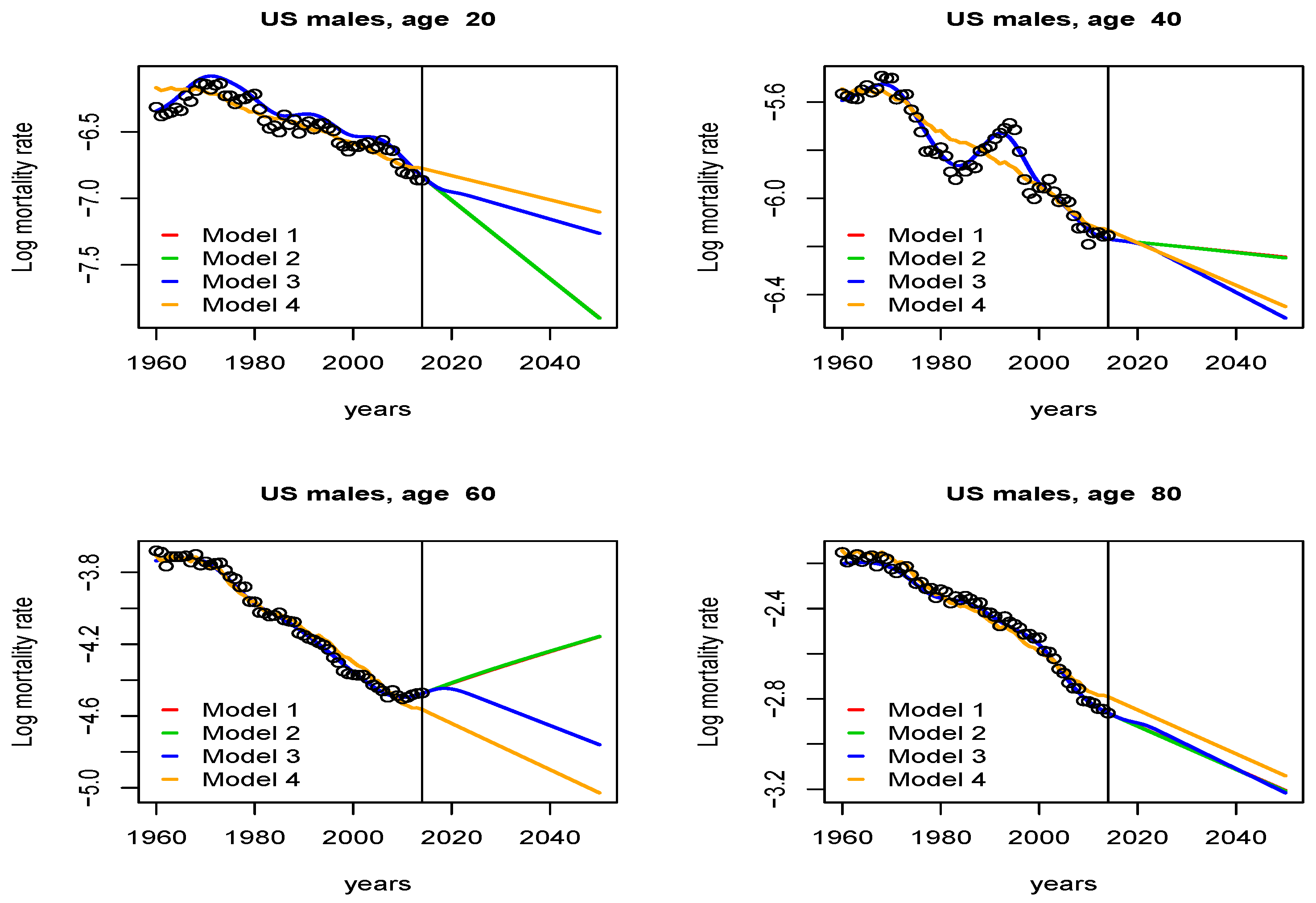
Figure 1 shows the fit and the forecast obtained with all four models. In order to highlight the difference between the results, we have selected four ages: 20, 40, 60, and 80. Figure 2 shows the fit and forecast for these ages obtained by model 1 (red line), model 2 (green line), model 3 (blue line) and model 4 (orange line). The first three models (models 1, 2 and 3) provide almost the same fit. However, the fit given by model 4 is quite different and worse than the fits of other models, at 20 and 40 years. This is to be expected because the Lee–Carter model is not flexible enough to capture the increase in mortality in the early 1980s.
The predictions with models 1 and 2 are almost identical. Although it gave very similar results in the fitting, model 3 provided completely different results in the predictions, as expected. For 60 years of age, model 1 and model 2 predict that the logarithmic death rate will increase during 2020–2050, because they predict an upward trend in death rates from 2010 to 2014. This is inconsistent with the expected result. In the case of model 4, forecasts are close to model 3 for ages 40 and 80, but in the case of age 20 it seems to clearly overestimate the mortality. In model 3, the increasing trend is corrected after the initial years to maintain the structure of the adjacent ages, thus avoiding irregular predictions (as happens at age 60).
As we have seen, when we impose the two constraints, we obtain the most realistic results: maintain the fit and the cross-age structure, that is, those given by model 3. If we do not maintain the coefficient pattern, age crossover may occur. We further illustrate this fact in Figure 3, we plot the projections obtained with model 2 (green line) and model 3 (blue line) for ages 66 and 67. We can see that the fit of the two models is the same, and within the known data range, the log mortality of age 66 is lower than that of age 67. However, in the forecast, model 2 does not avoid the cross-over for ages 66 and 67 and so, in 2050, the log mortality rate is larger for age 66 than for age 47, this cross-over is not biologically acceptable since it is expected that mortality rates of older people are higher. This does not occur with model 3 where the restrictions imposed preserve the cross-age structure among ages.
3. Component-Wise Prediction with P-Spline Smooth-ANOVA Models
In some cases, the multidimensional model in (1) is not flexible enough, and it may result in unnecessary complex models (that is, use too many degrees of freedom to fit the data). In order to add more flexibility and avoid unnecessary and irrelevant terms, the authors of [8] propose the use of P-spline smooth-ANOVA models (or S-ANOVA). This method decomposes the sum of smooth functions in a similar way to the analysis of variance decomposition, i.e., main and interaction effects. In this section, we will show how to obtain out-of-sample predictions in this setting. First, we briefly review how to fit the S-ANOVA model and show how the P-spline mixed model representation can avoid the identifiability problem that occurs when multiple smoothing terms are used in the same model.
Suppose we have data laid out as a rectangular array, and is the response vector of length , where , and and are the covariates. Let us consider the following S-ANOVA model:
where , i.e., the errors are independent and identically distributed and the B-spline basis is defined as:
of dimension , and where and are column vectors of ones of length and respectively, and the vector of regression coefficients are , where and are the vectors of coefficients for the main effects, of dimension and , respectively, and is the vector of coefficients for the interaction, of dimension . Therefore, model (31) is written as:
with penalty equal to the following block-diagonal matrix:
of dimension , where each block corresponds to the penalty over each set of coefficients in the model. Ref. [15] pointed out that model (33) and penalty (34) should be modified in order to preserve identifiability. Their proposal is to construct identifiable bases and penalties by reparameterizing the model as a mixed model instead of imposing numerical constraints as suggested by [18]. Ref. [15] defines the following transformation matrix with dimension , where:
and and are the eigenvectors corresponding to the positive values of the SVD of the marginal penalties, and , and and are the second columns of and , respectively.
Given the previous transformation matrix, ref. [15] showed that the fixed and random effects matrices and are:
where , , and . Moreover, the mixed model penalty (or equivalently, the precision matrix of random effects) is:
where for a second order penalty, it has size , and with:
where and are the nonzero eigenvalues of the SVD of and , respectively. Then, model (31) becomes:
With the previous representation of model (31), ref. [15] avoid the identifiability problem removing the column vector of s in the random effects matrix (38). For more details, see [15].
Although the out-of-sample prediction will be performed in the context of a mixed model, we introduced the method in the original P-spline formulation because the reparameterization required for out-of-sample prediction will be based on this definition. In particular, we need to know the extended penalty matrix in order to calculate the precision matrix of random effects.
In model (31), given a vector of observations of the response variable, suppose that we want to predict new values at , and of observed and predicted values can be arranged as in (20). Then, we consider the following extended smooth-ANOVA model:
where is defined as in (10) with an extended B-spline basis defined as:
of dimension , and where and are column vectors of ones of length and , respectively.
Therefore, model (40) is written as:
with extended penalty the following block-diagonal matrix:
of dimension , where each block corresponds to the penalty over each of the coefficients of the model.
In order to reformulate the extended S-ANOVA model (40) as a mixed model, we need to define an extended transformation matrix. The obvious choice would be to use the natural extended transformation matrix based on the SVD of the extended difference matrices; however, this method cannot ensure the invariance of the fit when performing out-of-sample predictions. In the following section, we propose the use of an extended transformation matrix, , that ensures coherent predictions.
3.1. Coherent Prediction with S-ANOVA Model
In order to use the S-ANOVA model for prediction under the constraint that the fit must be maintained, an extended transformation matrix that preserves the model matrix must be used. When the two covariates are extended, we define the following extended transformation matrix with dimension , and:
where and are the second columns of and , respectively,
are the eigenvectors corresponding to the positive values of the SVD of and and are blocks of (14). , , and have analogous definitions. Then, the fixed effects matrix is:
where and are and , respectively, and the random effects matrix is:
where and are and , respectively. The covariance matrix of random effects is , with given by the following theorem.
Theorem 2.
The extended precision matrix of the random effects for S-ANOVA model in (40) with extended transformation matrix given in (45), and extended penalty given in (43), is a block-diagonal matrix given by:
where:
with
The proof is given in the Supplementary Materials.
3.2. Example 2: Prediction of Aboveground Biomass
In this section, we apply the proposed 2D interaction P-spline and S-ANOVA models to another real data sets. The data come from an agricultural experiment conducted in Spain [19] to evaluate the economic viability of Populus trees prior to harvesting. In this context, it is important to estimate the aboveground biomass and obtain accurate predictions using only a minimal set of readily available information, i.e., diameter and height (denoted by and ). Ref. [20] proposed the use of smooth additive mixed models for predicting aboveground biomass. Here, we analyzed the data of one of the nine clones included in the experiment. The observation data consist of 315 observations for the diameter value measured at a breast height of 1.30 m. The data are shown in Figure 4, where it can be seen that the weight is a nonlinear function of diameter and height. We propose predicting out-of-sample aboveground biomass as a smooth function of height and diameter using the following two models:
- 2D interaction P-spline model:
- Smooth-ANOVA model:
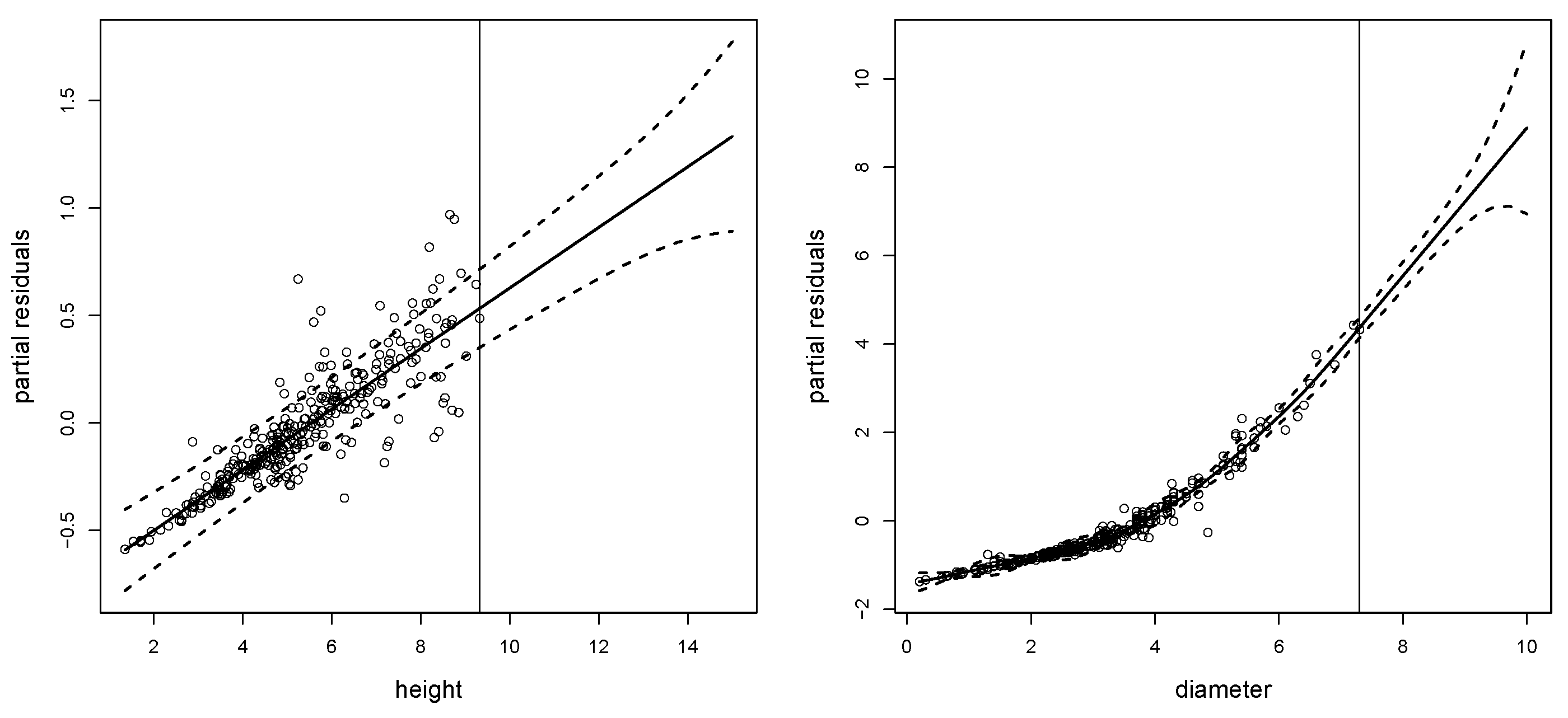
We have predicted weights for 10 new out-of-sample values for diameter and height. In Figure 5, we show the estimated smooth main effects for height (left panel) and diameter (right panel) obtained after fitting and predicting with the S-ANOVA model imposing that the fit is maintained. As shown, the effect of height is weaker than diameter, but both smooth terms are significantly different from zero. Figure 6 shows the fitted and predicted interaction function () for the restricted S-ANOVA model.
Figure 7 shows the predictions when the fit and the forecast are obtained with the S-ANOVA model (top left panel), with the S-ANOVA model subject to the constraint that the fit is maintained (top right panel), with the 2D interaction P-spline model (bottom left panel) and with the 2D interaction P-spline models imposing that the fit is maintained (bottom right panel). As shown in the figure, the results obtained by the S-ANOVA model and the restricted S-ANOVA model are almost equal. However, the solution obtained from the 2D interaction P-spline model is different depending on whether the constraint of maintaining the fit is imposed. However, the solutions obtained from the 2D interaction P-spline models are different depending on whether the restriction the fit is maintained is imposed or not. In particular, if no constraints are imposed, the fit will change significantly.
In the prediction, the most significant difference is that weight values predicted by the 2D interaction P-spline model at the largest diameter and height values are lower than the ones obtained by the S-ANOVA model. It is important to note that, in the fit, the degrees of freedom are 32 for the 2D interaction P-spline model and 12 for the S-ANOVA model, i.e., with the 2D interaction P-spline model, we are adding unnecessary complexity.
Furthermore, comparing the S-ANOVA model and the 2D interaction P-spline model, we conclude that the S-ANOVA model gives the most coherent solution because it provides the largest weight value for the highest values of height and diameter.
4. Simulation Study
We propose two simulation studies to examine the performance of the interaction 2D model and smooth-ANOVA model compared to their constrained versions (imposing the invariance of the fit when performing out-of-sample predictions). For this propose we have simulated the data in two different scenarios:
- (a)
- Scenario 1. From an interaction model:
- (b)
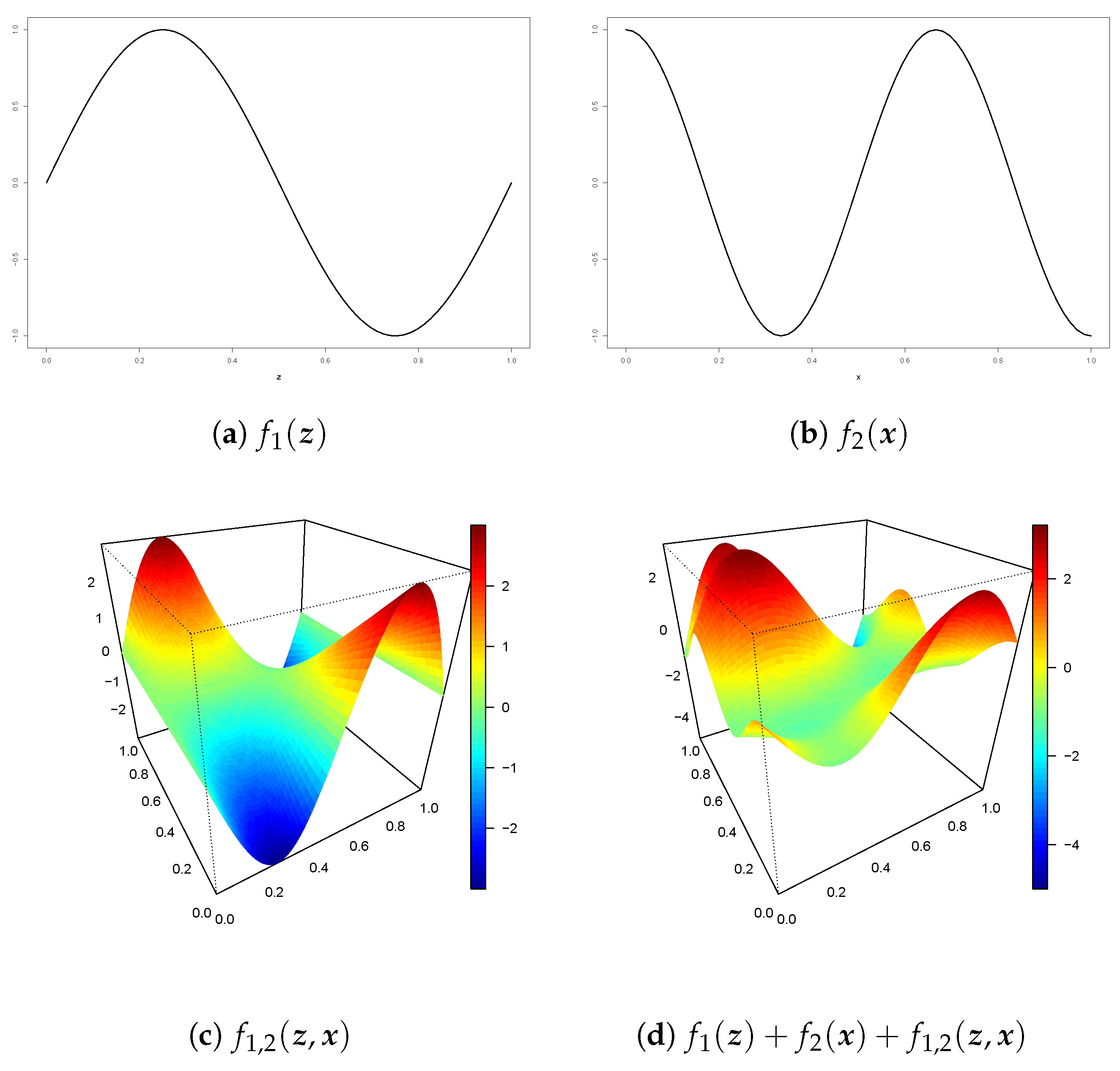
- Scenario 2. From a two main effects with interaction model:where , and . To simulate the data, we have generated a grid of 4900 values. Both covariates, and , take 70 equidistant values in the interval , and the errors are i.i.d., with mean 0 and variance . Figure 8 shows , and the surfaces proposed in scenarios 1 and 2.
The models compared are:
- 2D interaction P-spline model, i.e.,
- Smooth-ANOVA model, i.e.,
- Constrained 2D interaction P-spline model;
- Constrained smooth-ANOVA model.
The constraint imposed is that the coefficients of the fit remain invariant when out-of-sample-prediction is performed. In all cases, smoothing parameters are estimated using REML.
For each scenario and each model, we repeated the following steps 100 times:
- (1)
- Start with a data set of observations arranged into a matrix of dimension :where , , and have dimensions , , and , respectively;
- (2)
- Split our data into two groups: the training data and the test data , and ;
- (3)
- Use the training data to predict new observations ();
- (4)
- Check the accuracy of each model.
The marginal B-spline bases and are constructed with 15 knots and cubic splines and then extended to cover the whole range of and , the penalty orders are two.
As is known, a model that fits the data well does not necessarily yields good predictions, so we compared the fit performance, the forecast performance, and the overall method performance. In order to check the accuracy of the methods proposed, we followed [21] and used the difference between the function values from which we simulated the data and the fit and forecast produced using only the data in the training set:
i.e, we have the errors matrix and therefore the vectors containing the errors in the fit, in the forecast and in the overall performance:
- Vector with the fit errors: ;
- Vector with the prediction errors: ;
- Vector with the total errors: .
The errors measure that we use is the mean absolute error because, as it is concluded in [21], it is less sensitive to outliers than the root mean square error.
Mean absolute error: MAE =
for , i.e., for the errors in the fit, in the forecast or in total.
4.1. Simulations Results for Scenario 1
Here, we present results from Scenario 1. We use different ranges for the out of sample prediction, and fit and predict simultaneously with the four models described above. Note that for the different values of and we consider as the training data an observations matrix of dimension and we predict new values.
In Figure 9, we report MAE values from the fit, the forecast, and the overall performance. The x-axis label of boxplots refers to the model: unrestricted(2D interaction P-spline model), restricted (2D interaction P-spline model with constraints), ANOVA (S-ANOVA Model) and restricted S-ANOVA (S-ANOVA model with constraints).
Plots for the different values of and are available in the Supplementary Materials, and below we show the particular case of and .
In most cases, the fit remains relatively invariant in the case of the 2D P-spline models, with and without constraints, and in the restricted S-ANOVA model, while the fit in unrestricted S-ANOVA model is modified in most scenarios.
In the prediction, the three models behave similarly; however, the performance of the restricted S-ANOVA model is a bit worse and its MAE error values increase with an increasing prediction horizon (see Figures S1 and S2 of the Supplementary Materials).
Based on this simulated scenario, we conclude that simultaneous fit and prediction with S-ANOVA models produces significant changes in the fit and that in the overall performance (including fit and prediction), the 2D P-spline models (with and without restriction) and the restricted S-ANOVA models are the most accurate.
4.2. Simulations Results for Scenario 2
In the Supplementary Materials (Figure S12), we show the results obtained for Scenario 2, i.e., in the case in which the true surface is constructed from a model with two main effects and an interaction. Figure 10 shows the boxplots for the particular case of and .
In this case, the conclusion is that there is a significant difference between the results obtained with the interaction models and the S-ANOVA models: two-dimensional P-spline models (restricted and unrestricted) are always less accurate than the S-ANOVA models. This is due to the fact that 2D interaction models try to fit the data without considering the main effects.
When fitting the observed data, the performance of 2D P-spline interaction models, with and without constraints, is quite similar. However, the restricted interaction model is better than the unrestricted model in the out-of-sample prediction, the difference between the two models is apparent for most scenarios.
In the case of the S-ANOVA models, the restricted model is always better than the unrestricted one, in the fit, in the prediction and, therefore, in the overall performance. Although, in the particular case in which we only predict in one dimension, the prediction errors for both models are almost equal (see Supplementary Materials, scenario 2). The conclusion for this scenario is that the restricted S-ANOVA model is clearly the most accurate.
Therefore, considering all test scenarios, our recommendation is that, as a general rule, restricted S-ANOVA models should be used to fit and predict models that require interaction terms.
5. Conclusions
In this article, we propose a general framework for out-of-sample prediction in a smooth additive model with interaction terms. We build our proposal from the method proposed in [10], and then we extend their method to situations where out-of-sample predictions are required in both directions of the interaction term. The method proposed in [10] considers out-of-sample predictions as missing values with a weight of 0, and performs fitting and prediction at the same time. We have shown that this method produces different fitted values, depending on whether we only fit or fit and predict simultaneously.
In order to solve this inconsistency, we recommend maximizing the penalized likelihood under linear constraints to ensure that the coefficients obtained in the data fitting remain unchanged when the fitting and out-of-sample prediction are performed at the same time. For this purpose, we use Lagrange multipliers. This general method can be used to impose other related constraints, such as mortality forecasting when the cross-age structure needs to be preserved.
The methodology proposed has been extended to the case of smooth mixed models since it will allow us to predict out-of-sample in a wide range of models. We have shown that care should be taken when formulating the models as mixed models, since the matrices of fixed and random effects for out-of-sample prediction need to be direct extensions of the matrices used in the fit. In this context, we have developed a method for out-ofsample prediction for the S-ANOVA model proposed in [8]. This is an important step forward since, until now, there was no general method available for prediction in models that include main effects and interactions terms. A simulation study has been carried out to compare restricted and unrestricted out-of-sample predictions when using 2D interaction models and S-ANOVA models. From the results of the simulation study, we conclude that, in most cases, when the prediction is made on the two dimensions of the interaction term, the restricted S-ANOVA model performs better in fitting and out-of-sample prediction. The results for only one of the covariates depends on the simulation scenario, although in most cases, the S-ANOVA model is better than the full interaction (restricted or unrestricted) model.
The multidimensional prediction P-splines method with constraints proposed has also been used in two real data examples, one in which mortality rates are forecasted over the years, and the importance of imposing constraints on the coefficients to ensure coherent forecast is shown. The other example predicts tree biomass as a function of the tree height and diameter using the S-ANOVA model; this example shows the ability of this model to produce separate out-of-sample predictions for main effects and interaction terms in the model. Although here, due to the nature of the data used, we have only shown examples of forward out-of-sample prediction, our methodology allows for backwards out-of-sample predictions.
Currently, the work presented here is being extended to non-Gaussian responses in the context of generalized additive and mixed models.
Supplementary Materials
The following are available online at https://0-www-mdpi-com.brum.beds.ac.uk/article/10.3390/math9151761/s1 with Proof of theorem 1 and Corollary of theorem 1; Proof of theorem 2; Figures S1–S11 contains additional settings for the parameters in scenario 1; Figures S12–S21 contains additional settings for the parameters in scenario 2.
Author Contributions
Conceptualization, A.C., M.D. and D.-J.L.; methodology, A.C., M.D. and D.-J.L.; software, A.C.; validation, A.C.; formal analysis, A.C., M.D. and D.-J.L.; investigation, A.C., M.D. and D.-J.L.; resources, M.D. and D.-J.L.; data curation, M.D.; writing—original draft preparation, A.C.; writing—review and editing, M.D. and D.-J.L.; visualization, D.-J.L.; supervision, M.D. and D.-J.L.; project administration, M.D. and D.-J.L.; funding acquisition, M.D. and D.-J.L. All authors have read and agreed to the published version of the manuscript.
Funding
This research was funded in part by Ministerio de Ciencia e Innovación grant numbers PID2019-104901RB-I00. The third author gratefully acknowledges support by the Department of Education, Language Policy and Culture from the Basque Government (BERC 2018-2021 program), the Spanish Ministry of Economy and Competitiveness MINECO and FEDER: PID2020-115882RB-I00/AEI/10.13039/501100011033 funded by Agencia Estatal de Investigación and acronym “S3M1P4R”, and BCAM Severo Ochoa excellence accreditation SEV-2017-0718).
Institutional Review Board Statement
Not applicable.
Informed Consent Statement
Not applicable.
Data Availability Statement
Mortality data are openly available in the Human Mortality Database https://www.mortality.org (accessed on 1 July 2021). Biomass data are not available due to confidentiality issues.
Conflicts of Interest
The authors declare no conflict of interest.
References
- Eilers, P.H.C.; Marx, B.D. Flexible smoothing with B-splines and penalties. Stat. Sci. 1996, 11, 89–121. [Google Scholar] [CrossRef]
- Eilers, P.H.C.; Marx, B.D.; Maria, D. Twenty years of P-splines. Stat. Oper. Res. Trans. 2015, 39, 149–186. [Google Scholar]
- Li, Y.; Ruppert, D. On the asymptotics of penalized splines. Biometrika 2008, 95, 415–436. [Google Scholar] [CrossRef]
- Xiao, L. Asymptotic theory of penalized splines. Electron. J. Stat. 2019, 13, 747–794. [Google Scholar] [CrossRef]
- Wand, M. Smoothing and mixed models. Comput. Stat. 2003, 18, 223–249. [Google Scholar] [CrossRef]
- Kauermann, G. Penalized splines, Mixed Models and Bayesian Ideas. In Statistical Modelling and Regression Structures: Festschrift in Honour of Ludwig Fahrmeir; Physica-Verlag: Heidelberg, Germany, 2010; pp. 45–58. [Google Scholar] [CrossRef]
- Currie, I.D.; Durbán, M.; Eilers, P.H.C. Generalized linear array models with applications to multidimensional smoothing. J. R. Stat. Soc. Ser. B 2006, 68, 1–22. [Google Scholar] [CrossRef]
- Lee, D.J.; Durbán, M. P-spline ANOVA-type interaction models for spatio-temporal smoothing. Stat. Model. 2011, 11, 49–69. [Google Scholar] [CrossRef] [Green Version]
- Lee, D.J.; Durbán, M.; Eilers, P.H.C. Efficient two-dimensional smoothing with P-spline ANOVA mixed models and nested bases. Comput. Stat. Data Anal. 2013, 61, 22–37. [Google Scholar] [CrossRef]
- Currie, I.D.; Durbán, M.; Eilers, P.H.C. Smoothing and forecasting mortality rates. Stat. Model. 2004, 4, 279–298. [Google Scholar] [CrossRef]
- Etxeberria, J.; Ugarte, M.; Goicoa, T.; Militino, A.F. On predicting cancer mortality using anova-type P-splines models. Rev. Stat. J. 2015, 13, 21–40. [Google Scholar]
- Ugarte, M.D.; Goicoa, T.; Etxeberria, J.; Militino, A.F. Projections of cancer mortality risks using spatio-temporal P-spline models. Stat. Methods Med. Res. 2012, 21, 545–560. [Google Scholar] [CrossRef] [PubMed]
- Carballo, A.; Durban, M.; Kauermann, G.; Lee, D.J. A general framework for prediction in penalized regression. Stat. Model. 2020. [Google Scholar] [CrossRef]
- Greene, W.H.; Seaks, G.T. The Restricted Least Squares Estimator: A Pedagogical Note. Rev. Econ. Stat. 1991, 73, 563–567. [Google Scholar] [CrossRef]
- Lee, D.J. Smoothing Mixed Models for Spatial and Spatio-Temporal Data. Ph.D. Thesis, Department of Statistics, Universidad Carlos III de Madrid, Madrid, Spain, 2010. [Google Scholar]
- Lee, R.; Carter, L. Modelling and forecasting the time series of US mortality. J. Am. Stat. Assoc. 1992, 87, 659–671. [Google Scholar]
- Delwarde, A.; Denuit, M.; Eilers, P.H.C. Smoothing the Lee-Carter and Poisson log-bilinear models for mortality forecasting: A penalized log-likelihood approach. Stat. Model. 2007, 7, 29–48. [Google Scholar] [CrossRef]
- Wood, S. Low-rank scale-invariant tensor product smooths for generalized additive mixed models. Biometrics 2006, 62, 1025–1036. [Google Scholar] [CrossRef] [PubMed] [Green Version]
- Rivas-Martínez, S.; Díaz, T.E.; Fernández-González, F.; Izco, J.; Loidi, J.; Lousã, M.; Penas, A. Vascular plant communities of Spain and Portugal. Addenda to the syntaxonomical checklist of 2001. Itinera Geobot. 2002, 15, 5–922. [Google Scholar]
- Sánchez-González, M.; Durbán, M.; Lee, D.; Cañellas, I.; Sixto, H. Smooth additive mixed models for predicting aboveground biomass. J. Agric. Biol. Environ. Stat. 2016, 22, 23–41. [Google Scholar] [CrossRef] [Green Version]
- Hyndman, R.J.; Koehler, A.B. Another look at measures of forecast accuracy. Int. J. Forecast. 2006, 22, 679–688. [Google Scholar] [CrossRef] [Green Version]
Figure 1.
Fit and forecast of a data set on the log mortality rates of US males aged 0–110+ over the period 1960–2014, through model 1 (top left), model 2 (top right), model 3 (bottom left) and model 4 (bottom right). The horizontal line indicates the year from which we predict (2014).
Figure 1.
Fit and forecast of a data set on the log mortality rates of US males aged 0–110+ over the period 1960–2014, through model 1 (top left), model 2 (top right), model 3 (bottom left) and model 4 (bottom right). The horizontal line indicates the year from which we predict (2014).

Figure 2.
Fit and forecast of selected ages: 20, 40, 60 and 80 obtained using model 1 (red line), model 2 (green line), model 3 (blue line) and model 4 (orange line). The vertical line indicates the year from which we predict (2014).
Figure 2.
Fit and forecast of selected ages: 20, 40, 60 and 80 obtained using model 1 (red line), model 2 (green line), model 3 (blue line) and model 4 (orange line). The vertical line indicates the year from which we predict (2014).

Figure 3.
Fit and forecast for ages 66 and 67 obtained through model 2 (green line) and model 3 (blue line). Model 3 prevent cross-over for ages. The vertical line indicates the year from which we predict (2014).
Figure 3.
Fit and forecast for ages 66 and 67 obtained through model 2 (green line) and model 3 (blue line). Model 3 prevent cross-over for ages. The vertical line indicates the year from which we predict (2014).

Figure 4.
Plot of weight versus height (left) and plot of total weight versus diameter (right).

Figure 5.
Fitted and predicted smooth curves for height (left) and for diameter (right) using the restricted S-ANOVA model. The vertical line indicates the height and diameter values from which we predict (9.32 and 7.3).
Figure 5.
Fitted and predicted smooth curves for height (left) and for diameter (right) using the restricted S-ANOVA model. The vertical line indicates the height and diameter values from which we predict (9.32 and 7.3).

Figure 6.
Fitted and predicted interaction function for the the restricted S-ANOVA model. The vertical line indicates the height value from which we predict (9.32) and the horizontal line indicates the diameter value from which we predict (7.3).
Figure 6.
Fitted and predicted interaction function for the the restricted S-ANOVA model. The vertical line indicates the height value from which we predict (9.32) and the horizontal line indicates the diameter value from which we predict (7.3).

Figure 7.
Fit and prediction with the S-ANOVA model (top left), with the S-ANOVA model, imposing that the fit is maintained (top right), with the 2D interaction P-spline model (bottom left) and with the 2D interaction P-spline models imposing that the fit is maintained (bottom right) at out-of-sample values of diameter [7.3,10] and height [9.32,15].

Figure 8.
Functions (a,b) are the nonlinear main effects of z and x, (c) is the interaction surface and (d) is the sum of the main effects and the interaction surfaces.
Figure 8.
Functions (a,b) are the nonlinear main effects of z and x, (c) is the interaction surface and (d) is the sum of the main effects and the interaction surfaces.

Figure 9.
MAE in the fit (left), in the forecast (middle) and in total (right) of smooth models in scenario 1 and nzp = 0 and nxp = 5.
Figure 9.
MAE in the fit (left), in the forecast (middle) and in total (right) of smooth models in scenario 1 and nzp = 0 and nxp = 5.

Figure 10.
MAE in the fit (left), in the forecast (middle) and in total (right) of smooth models in scenario 2 and nzp = 0 and nxp = 5.
Figure 10.
MAE in the fit (left), in the forecast (middle) and in total (right) of smooth models in scenario 2 and nzp = 0 and nxp = 5.

Publisher’s Note: MDPI stays neutral with regard to jurisdictional claims in published maps and institutional affiliations. |
© 2021 by the authors. Licensee MDPI, Basel, Switzerland. This article is an open access article distributed under the terms and conditions of the Creative Commons Attribution (CC BY) license (https://creativecommons.org/licenses/by/4.0/).
Share and Cite
MDPI and ACS Style
Carballo, A.; Durbán, M.; Lee, D.-J. Out-of-Sample Prediction in Multidimensional P-Spline Models. Mathematics 2021, 9, 1761. https://0-doi-org.brum.beds.ac.uk/10.3390/math9151761
AMA Style
Carballo A, Durbán M, Lee D-J. Out-of-Sample Prediction in Multidimensional P-Spline Models. Mathematics. 2021; 9(15):1761. https://0-doi-org.brum.beds.ac.uk/10.3390/math9151761
Chicago/Turabian StyleCarballo, Alba, María Durbán, and Dae-Jin Lee. 2021. "Out-of-Sample Prediction in Multidimensional P-Spline Models" Mathematics 9, no. 15: 1761. https://0-doi-org.brum.beds.ac.uk/10.3390/math9151761
Note that from the first issue of 2016, this journal uses article numbers instead of page numbers. See further details here.