
Impact Dynamics Analysis of Mobile Mechanical Systems

1
Faculty of Automation, Computers and Electronics, University of Craiova, 200776 Dolj, Romania
2
Faculty of Mechanics, University of Craiova, 200512 Dolj, Romania
*
Author to whom correspondence should be addressed.
Mathematics 2021, 9(15), 1776; https://0-doi-org.brum.beds.ac.uk/10.3390/math9151776
Submission received: 9 June 2021
/
Revised: 4 July 2021
/
Accepted: 19 July 2021
/
Published: 27 July 2021
(This article belongs to the Special Issue Dynamical Systems and Their Applications (DSTA) — In Memory of Prof. Dr. José A. Tenreiro Machado)
Abstract
:The current paper focuses on the impact phenomenon analysis, in the case of multi-body mechanical systems undergoing fast motion, due to the presence of some manufacturing and mounting errors or due to some accident during the transport mechanical systems. Thus, the impact phenomenon was analyzed in two cases, the first one consisting of a two bodies, namely, a free-fall body brought in contact with the other considered fixed in space and the second case, which is a complex one, when the analyzed bodies are components of a multi-body mechanical system. The research main objective is to analyze the impact generated between the two bodies through three methods, i.e., the analytical method, a virtual prototyping method accomplished with MSC Adams software and a method based on finite element analysis with Ansys and Abaqus software. A dynamic model of the impact force was developed, which allows to make a comparison of the numerical results obtained through the abovementioned methods. As a multi-body mechanical system, it was considered a mechanism from an internal combustion engine from which the radial clearance between the piston bolt and connecting rod head of the considered mechanism was analyzed.
1. Introduction
The impact phenomenon can be present in the case of multi-body systems and this can be generated by many causes such as mounting and manufacturing errors, discontinuities of kinematic parameters variation or critical situation (for example, vehicle collision, etc.). Vehicle collisions are much more complex than other impact phenomena occurring between the two bodies.
The impact analysis of multi-body systems is of paramount importance since at the impact moment, the system state variables are quickly modified and discontinuities inside of system velocities and accelerations appear. These discontinuities can lead to forces of high values, which vary in a very short period of time. By knowing these forces variation peaks, it is important to take them into account during the mechanical systems design.
Using the research reported in [1], the authors show that there are two methods for solving impact problems of multi-body mechanical systems. The first method is based on a model of a “continuous” contact-force type. Similar models were analyzed in [2] and they underpinned a spring-damper element. Other research like that in [3] uses a Hertzian model for impact analysis. The second method is used more frequently than the first one and this is called the piecewise analysis method, where the motion equations integration stops at the moment of impact.
The research data from [4] present an impact analysis for models with friction from mechanical systems, which contain open kinematic linkages. Two problem types, namely, a bar, which drops free on the ground and a double pendulum system in a free fall, are examined. Thus, by solving the analytical impact problem it can be remarked that this mainly depends on motion equation integration at three impact phases, i.e., before, during and after the impact. This it could be a starting point for the proposed research.
In the research reported in [5] information is provided on whether impact events of mechanical systems can be successfully modeled through simple or low-order finite elements. There are developed simple finite element models which are benchmarked against theoretical impact problems and published experimental impact results. A case study is also presented, a finite element model using simple plastic beam elements. This is further tested to predict stresses and deflections in an experimental structural impact. The established workflow can be transposed to other impact problems because the stress levels predicted by the FEA model were generally within 10% of measured values. This demonstrates that a finite element analysis characterized by simple or low ordered finite elements can be used as a valid engineering tool for a medium-sized manufacturer in developing analyses of mobile mechanical systems or for designing products exhibiting impact requirements.
Impact phenomena can be studied by using simple models, especially experimental ones. This can generate complex problems which are hard to analyze through analytical methods. For example, the methods used in [6] develop analytical and experimental studies on some models based on free-fall drop impact analysis of portable products similar to cell phones. Thus, the research core was represented by a developed simplified analytical procedure for obtaining the dynamic response during impact in case of a free fall dropped object. The developed experimental analysis uses special objects with accelerometers mounted inside. With the use of a special drop tower with a guiding frame for controlled-angle free-fall drop impact, the used objects are dropped at different angles and the acceleration during impact is recorded. The aim of this analysis is to improve the conceptual solutions for impact resistance of portable products. From this research the experimental infrastructure can be noted and for further research the principle can lead to the use of small objects presumed to undergo a free fall drop. Thus, an experimental stand can be elaborated and an accelerometer can be placed inside of the base component. Also for experimental tests video motion analysis with high speed cameras can be used for analyzing impact phenomena.
Impact phenomena occur in various domains and cases, starting from medicine, accidentology, mechanical engineering, civil engineering, military defense, food industry, chemistry or physics. From this different methods and tools can be extracted for impact modeling.
In [7] the civil engineering specialists analyzed the behavior of concrete specimens during impact phenomena. Thus, experimental tests were made by dropping a constant weight hammer from five different heights on concrete specimens placed on special cells equipped with accelerometers. The novelty of this research relies on a finite element model that is made by using the ABAQUS software. Thus, extra attention is paid to the modeling of impact incidence and a non-linear dynamic model was prepared. FEM in the presented research can only be used for giving designers a prior idea about the impact behavior. A similar analysis was conducted in [8] where the authors determined the most suitable drop height for shock testing military equipment. For this, an application of regression analysis and a back-propagation neural network for determining the most suitable drop height for free-fall shock tests was proposed. The mathematical model, elaborated through a regression analysis, was verified through a comparative analysis between experimental tests carried out on several military materials like specific elastomers in order to estimate the optimal height and duration for free-fall shock tests.
Based on free-fall drop objects, several experimental tests were performed in [9] by taking into account the related researches from [10,11,12,13]. The authors in [9] performed a quite modern experimental analysis of the impact-induced acceleration by obstacles with the use of flexible ball chains. It can be remarked that impact phenomena have different behavior and depend on various materials. The novel element is represented by the possibility of using modeling of discrete structures as continuous bodies with a complicated constitutive law of impact which includes angle of incidence as a starting point for the elaborated mathematical models.
Bearing in mind the research reported in [14,15] it can be remarked that impact phenomenon modeling can be performed through modern techniques and for these finite element modeling represents an essential tool. For example, in [14] a nonlinear dynamic finite element analysis for a cylinder piston model was performed. The authors developed finite element models analyzed under specific circumstances of collision impact with the ANSYS/LS-DYNA software. The developed mathematical model can be applied to mobile mechanical systems. Several input data for the developed numerical simulations are reported, but in this case the clearance between piston and cylinder was neglected. The obtained results are materialized through impact force under different velocities of the piston impact collar.
An important argument for controlling the input parameters for impact modeling relays on simple numerical simulations like the one reported in [15], where the developed numerical simulations examine the perforation of steel and aluminum plate specimens and then impact load is applied on composite plates with eight layers reinforced by carbon fibers. For this ABAQUS software was used for several numerical models of solid penetration i.e., Mohr-Coulomb model, Johnson-Cook model, Zerilli-Armstrong model, Steinberg-Guinam model and a thermo-mechanical material model. For these it is very important to retain the use of damping coefficient, penetration depth, restitution coefficient, and also the way of controlling the finite elements network.
The impact without friction was analyzed by other studies like those describe in [16,17,18,19]. In [20] contact-impact force models, with friction, for cylindrical surfaces and spherical ones are analyzed.
Based on the results reported in [21], a comparison between different contact-impact force models for a crank and connecting rod mechanism were made. In this research the major objective is to analyze the impact phenomena for two major cases:
- (1)
- Impact analysis for two bodies on a free-fall drop, which come in contact together, and
- (2)
- Impact study for a multi-body system from an internal combustion engine mechanism.
For the first case it is important to control the input data for numerical simulations in order to have better accuracy during impact phenomenon modeling. In the second case some input data from the previous case are reconsidered and the obtained results will improve the reliability of the mobile mechanical systems, especially the ones from internal combustion engines, but not limited to these.
The novel element achieved through this research is the numerical result accuracy based on the finite element method for studying a impact phenomena. In order to achieve this several contact analyses it will be proposed, namely with and without friction, with and without damping effect and for different dynamic impact force parameters. Another novel element is represented by the three impact modeling methods used, namely analytical, virtual prototyping and FEM analysis. These methods allow identifying the variation domain for important dynamic factors, namely penetration depth, damping coefficient and force application factor.
In a comparison with [6], the contact between two bodies on a free-fall drop will be better analyzed and controlled due to the mathematical considerations. This can be completed by using modern techniques implemented through finite element software. The desired data can be easily compared through experimental analyses conducted on similar models for analyzing impact phenomena.
2. Impact Analysis of a Link with Planar Surface
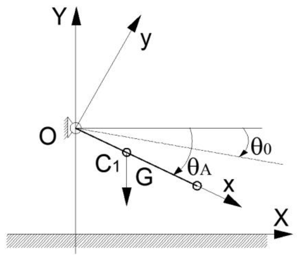
In this case, it will analyze a planar mechanical system made up of a bar with a circular cross-section, which will drop freely with one end on a planar surface, being articulated through a ball bearing joint at the other end, as it can be seen in Figure 1.
This bar has a transversal circular diameter of 4 mm and a length of 240 mm. The planar surface has a rectangular shape with a length of 300 mm, a width of 100 mm and a height of 6 mm. The envisaged bar link will drop free from a height of 194 mm.
For this model it is important to analyze the impact between the bar and the planar surface in three cases, namely, the analytical mode, modeling and numerical simulation with Adams software, the modeling with finite element method through the aid of ANSYS and Abaqus.
2.1. Analytical Method
The analytical method involved an elaborated mathematical model based on the kinematic scheme in Figure 1.
For the schematized model in Figure 1, it will obtain the bar angular speed from dynamics considerations:
where: G represents the bar weight, which actuates in the mass center C1; J0 is the mass inertia momentum depending on bar rotation center, O and is the bar rotation angle:
Equation (4) is integrated and it has the following form:
The initial conditions are introduced:
By introducing Equation (7) in (6) we obtain:
In addition, it will have the following mathematical expressions:
where: ω is the bar angular speed, l the bar length, and g the acceleration of gravity.
To determine the impact function, the displacement and speed of the free end of the bar, i.e., point (A), is considered. Therefore, the kinematic constraint equations are:
The generalized coordinate is: .
A proper Jacoby model for Equation (11) is:
Velocities
These will be obtained by differentiating the Equation (11) depending on time, and the obtained results are:
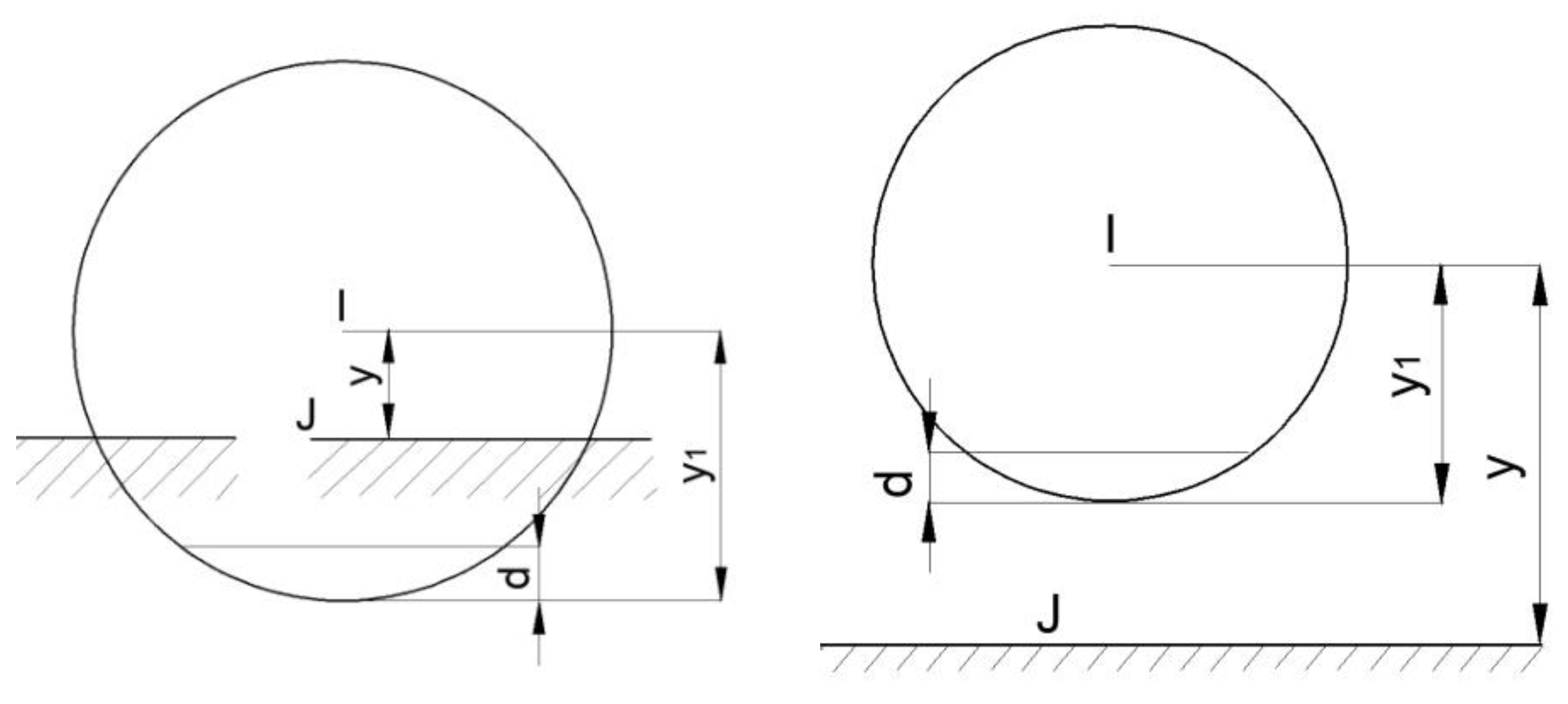
According to Figure 2, the impact function accepted by multibody systems theory [22] will have the following form:
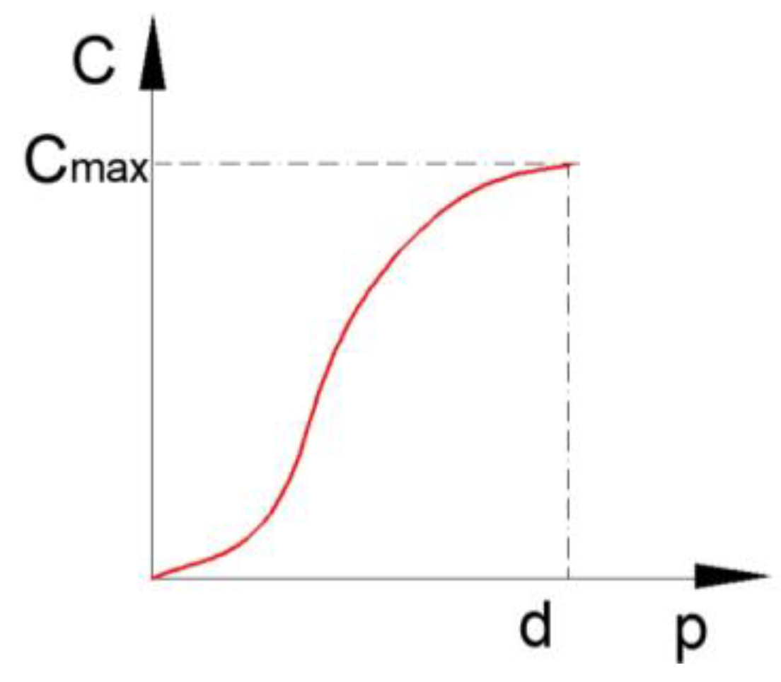
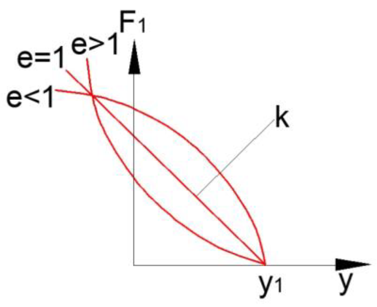
In Equation (14) one can identify the following terms: y—distance depending on time, which is necessary for the impact function calculus, namely: yA = yA(t); —the point speed at which it will consider that it will actuate the impact force, i.e., speed (point A speed); y1—a positive real variable, which can be considered to be the free length of y component displacement; k—stiffness which corresponds to the interaction between the bar and the contact surface; e—is a positive real variable which specifies the deformation characteristics exponent of the applied force; cmax—is a non-negative, double-precision variable that specifies the maximum damping coefficient; d—is a positive double-precision variable that specifies the secondary penetration at which ADAMS/Solver applies full damping.
The damping coefficient versus the penetration variation is plotted in Figure 3.
The stiffness term k, which can be seen in Equation (14), depends on material properties and the solid bodies’ radius when these get in contact together. This is calculated by using the following equation [22]:
where: Ri, Rj—represent the radii of each body in contact; νi, νj—represent the transversal contraction coefficients for bodies i and j brought in contact together; Ei, Ej—represent the longitudinal elasticity modulus for body i and body j, respectively.
It is important to know the following conditions:
- if y ≥ y1, there will be no penetration at the level of the contact surface, and in this case the impact force will be equal to zero (penetration p = 0);
- if y < y1, penetration occurs at the end closer to the i marker, and the impact force is >0 (penetration p = y1 − y);
- when p < d, the damping instantaneous coefficient is a cubic STEP function of penetration, labeled p;
- when p > d, the instantaneous damping coefficient will be cmax.
Thus, the impact function, regarding [22], has the following form:
The impact function is active when the distance between the markers i and j will be smaller than y1. Practically, this function enters when the considered bodies collide, otherwise, it will be equal to zero. Also, it will consider that the force in the mathematical expression of (14) has two components:
- a spring or stiffness component and a damping or viscous component:
Furthermore, the stiffness component will be an opponent term of penetration:
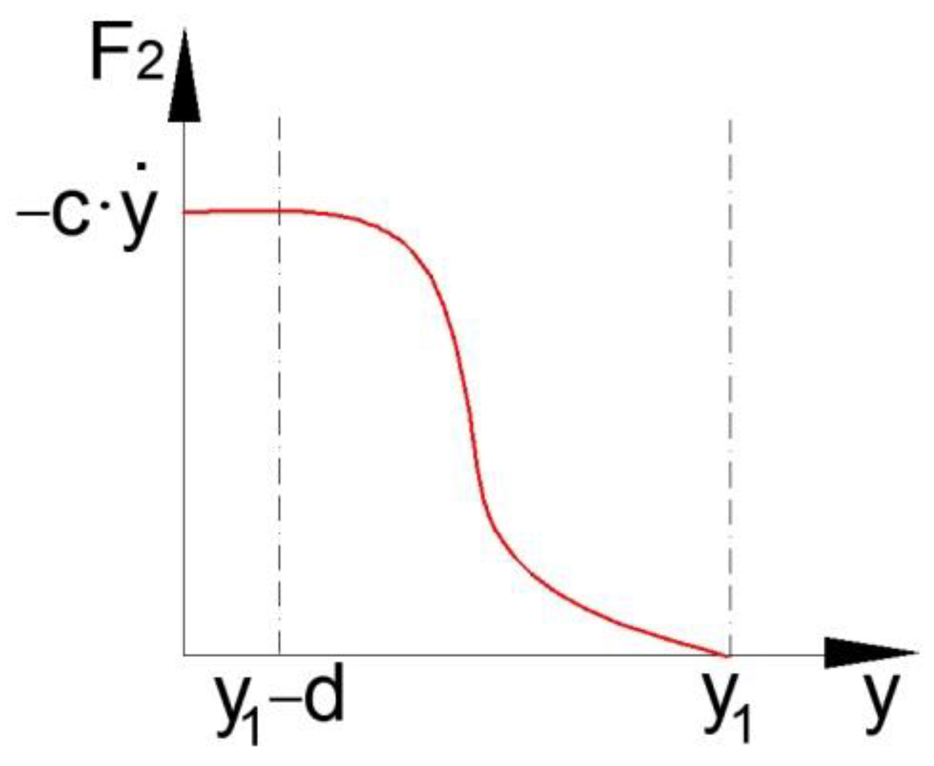
- damping (viscous component), which is a function of the speed of penetration.
Damping opposes the direction of relative motion. Alternatively, the mathematical model of the impact force, when the considered bodies collide, will be:
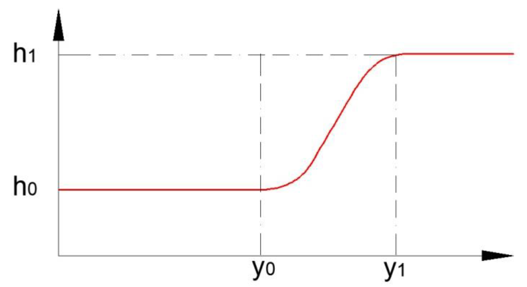
The STEP function approximates the Heaviside step function with a cubic polynomial one, as well as a STEP function, which looks like the one in Figure 6.
The equation by which a STEP function will be defined in the following form:
where:
Thus, the impact force mathematical model will be elaborated based on the mathematical expressions in Equation (14). For the proposed system presented in Figure 2, it will obtain: h0 is equal to zero for this aplication. By comparing Figure 5 and Figure 6, the mathematical expression (21) becomes:
where:
Thus, the k stiffness value can be calculated with Equation (15) and the obtained value will be k = 48,049. The presented mathematical models, which correspond to the impact force, can be numerically processed under MAPLE programming environment. Accordingly, the time intervals when the stiffness component and viscous component of impact force are actuated will be identified. These time intervals correspond to a programming sequence, namely Algorithm 1, with the MAPLE software as follows:
| Algorithm 1 Programming Sequence for Time Intervals |
| for t from 0 by 0.0001 to 0.6 do if print ; then print else print end if end do; |
Using the initial data and the programming sequence, the processing of the presented mathematical models will lead to the time variation diagrams of both impact force components. Two major cases defined through different damping coefficients will be considered:
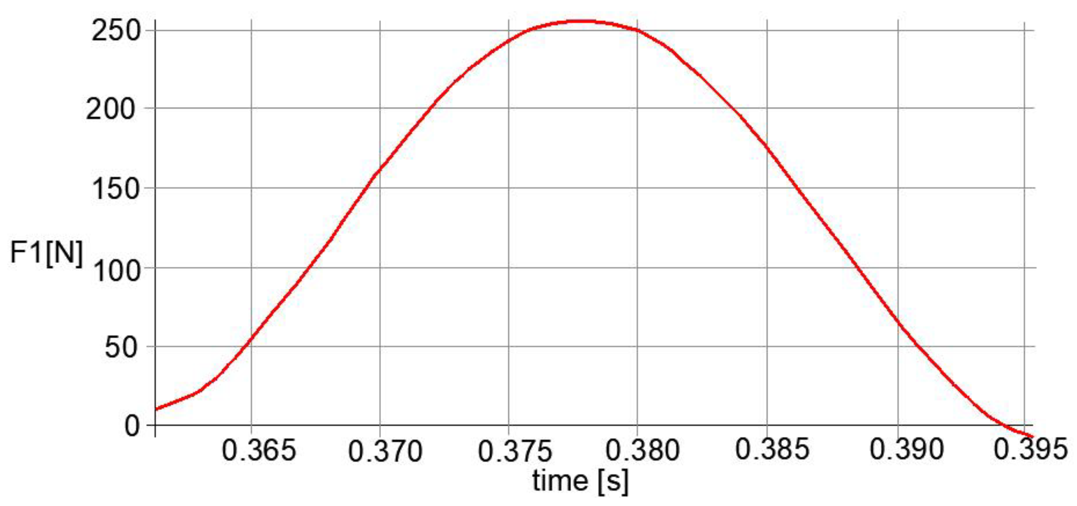
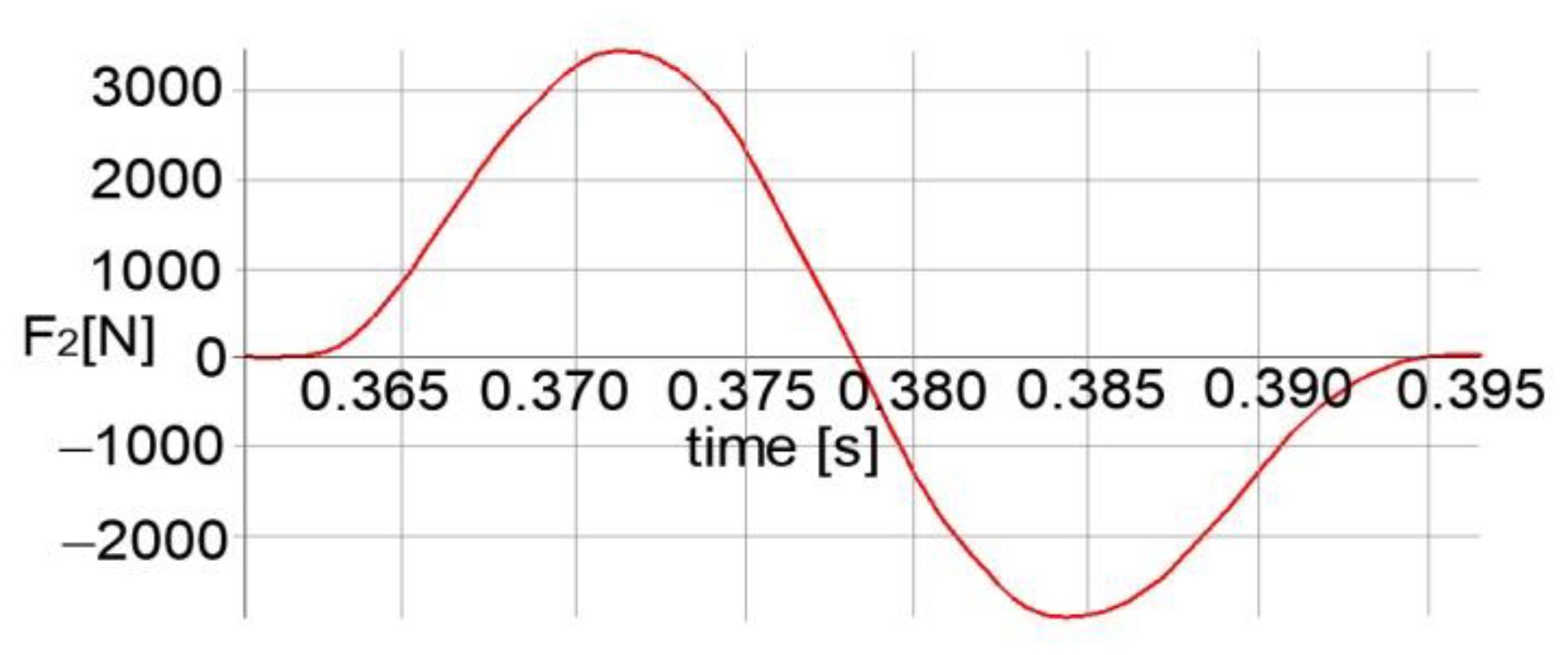
(a) Bar length: l = 240 mm; y1 = 0.8; damping coefficient: cmax = 1; penetration depth: d = 0.01; stiffness: k = 48,049; force exponent: e = 2.2. By considering the diagram in Figure 7, it can be noted that the impact force will have a maximum value of 250 N, and in Figure 8 the viscous component has a maximum value around 3000 N, and these values correspond to c = 1. If we modify the damping coefficient at a value of c = 6, the force stiffness component will reach a value of 450 N, according to Figure 9, and the viscous component reported in Figure 10 will reach a value of 5 × 10⁴ N.
(b) Bar length: l = 240 mm; y1 = 0.897; damping coefficient: cmax = 6; penetration depth: d = 0.01; stiffness: k = 48,049; force exponent: e = 2.2.
2.2. Impact Modeling with MSC Adams
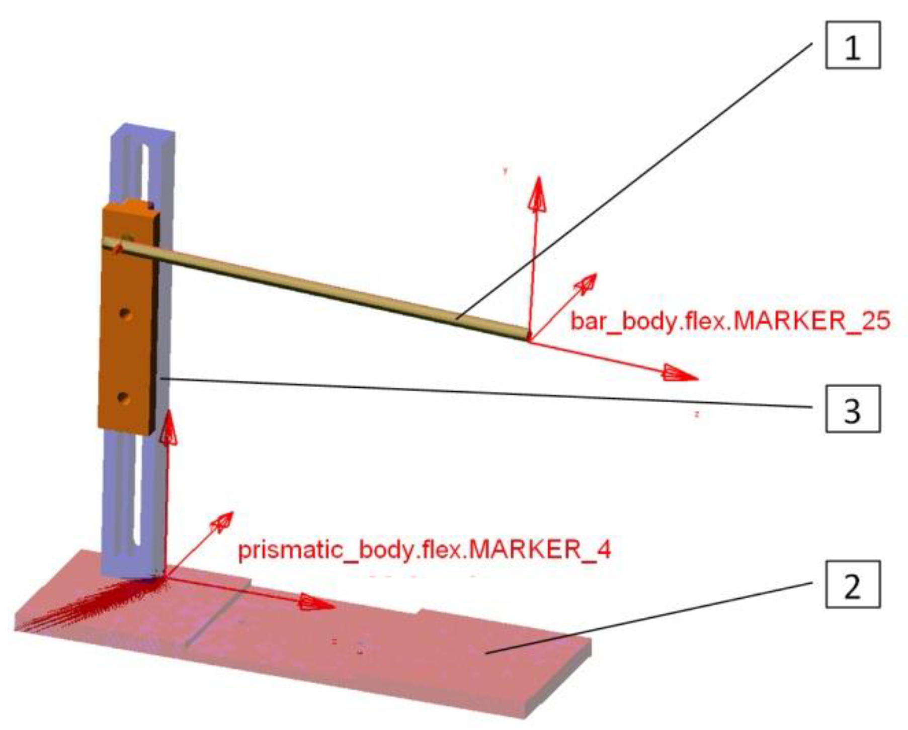
For the impact analysis, a virtual model was designed, equivalent to an experimental testbed, as can be observed in Figure 11. This contains in its structure a bar (1), a prismatic body (2) and a column composed of adjustable length devices (3). The considered bar has free motion on one end under its own weight. With the help of this virtual model the impact between the bar and the prismatic body will be analyzed. This will take place in three virtual environments, namely, MSC Adams, ANSYS and Abaqus software.
The virtual prototyping accomplished via the Adams program has on its background a kinematic model made up of five parts connected together through kinematic joints. Thus, the adjustable column (3) has devices which allow the user to adjust the drop height of the considered bar (1). By having a closer look at the impact between the abovementioned components from a dynamic viewpoint, these were defined as deformable bodies and were meshed with finite elements such as tetrahedral ones taking into account the connection between interest nodes.
To obtain the impact function corresponding to the elaborated dynamic model, the following steps are to be followed:
The marker which materializes the origin of the impact force (marker_25, in Figure 11) will be identified;
The kinematic parameters (displacements and velocities) for the application point of the impact force (displacement and velocity of marker 25 according to Figure 12) will be obtained through numerical simulations. These parameters are defined as functions depending on time;
The dynamic model parameters of the impact function, i.e., stiffness—k; damping—c; depth penetration—d; force exponent coefficient—e, will be evaluated.
The stiffness k will be calculated by Equation (15) by taking into account the geometry of the considered components which will be in contact together. The kinematic parameters are monitored in line with a local coordinate system, which is fixed with the prismatic body, defined through marker no. 4 (according to Figure 11).
The impact analysis of both component bodies will be made for two distinct cases, a contact made from rigid bodies and a contact made from deformable ones, respectively.
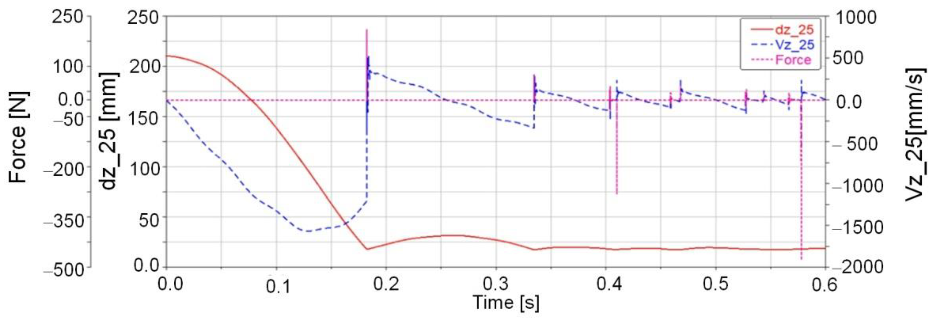
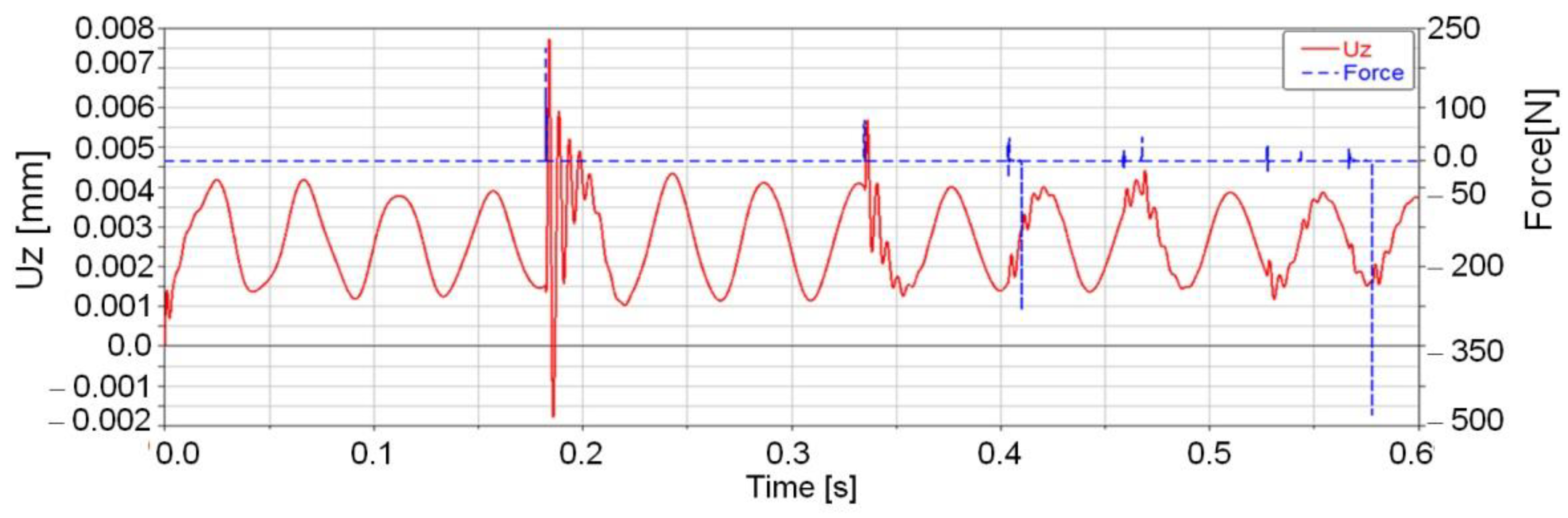
Thus, in Figure 12 the time variation laws for displacement in the case of marker no. 25 (dz_25), speed (vz_25) and impact force (force) can be seen. The dynamic parameters, which contribute to the impact function definition, have the following values: k = 48,049, e = 2.2, c = 1, d = 0.01. For differential equations integration the Adams solver GSTIFF I3 was used, with an integration step equal to 1 × 10⁻³. In addition, the recorded harmonics as amplitude and number obtained in the case of impact forces variation are generated mainly by the damping phenomenon.
In order to examine the prismatic body behavior at the contact moment with the bar, it is necessary to perform a transversal elastic displacement analysis of this, as shown in Figure 13. Thus, in Figure 13 the prismatic body elastic displacement and the impact force when the damping coefficient is equal to 1 are represented. It can be remarked that the elastic displacement is relatively small, whereas the impact force reaches maximum values.
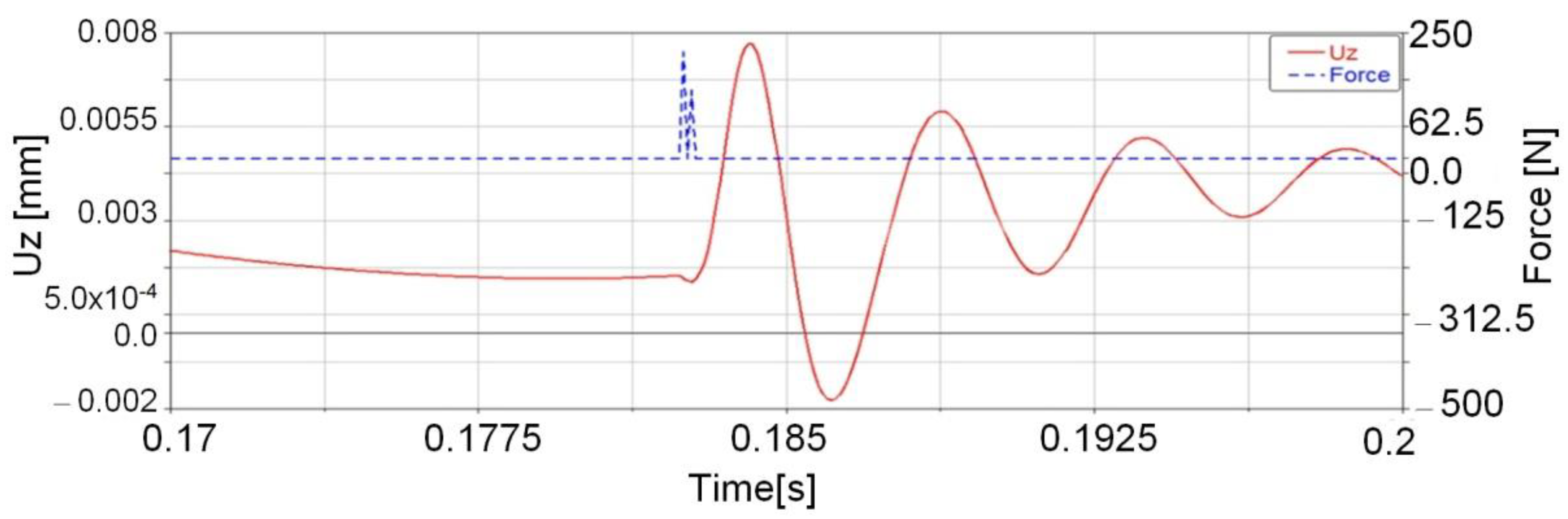
By considering Figure 14 and Figure 15, it can be observed that the impact force and displacement variation occur at the same time intervals. In this case, the contact number between the bar and the prismatic body is smaller than in the previous case.
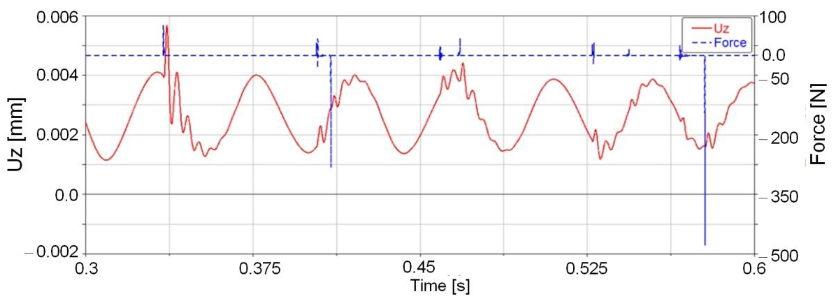
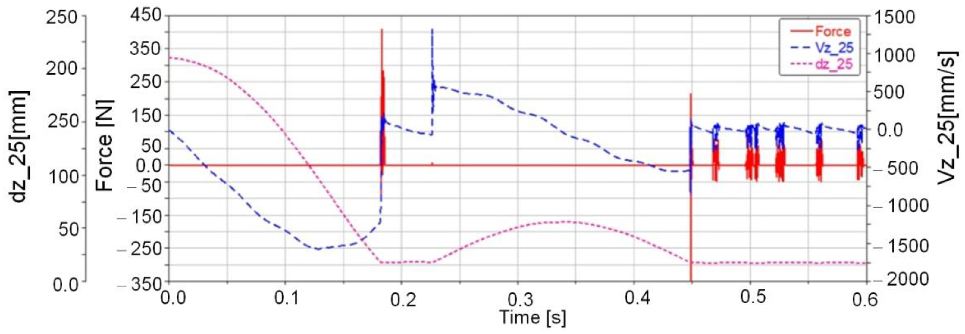
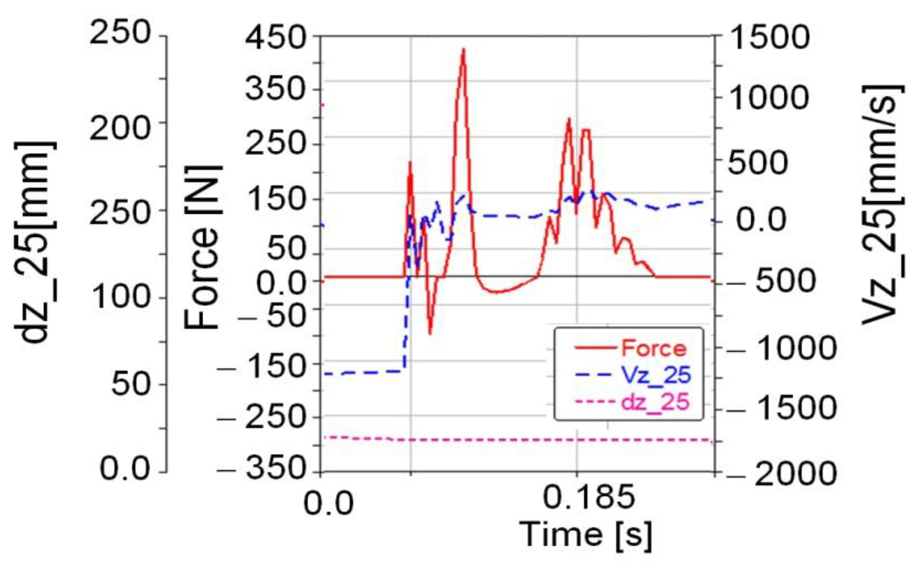
In Figure 16 and Figure 17, the impact force, displacement and speed variation diagrams of the analyzed marker, namely, marker no. 25 (dz_25, vz_25) are shown, when the damping coefficient is equal to c = 6. These diagrams were obtained by taking into account a local coordinate system placed on the prismatic body in marker no. 4, according to Figure 11.
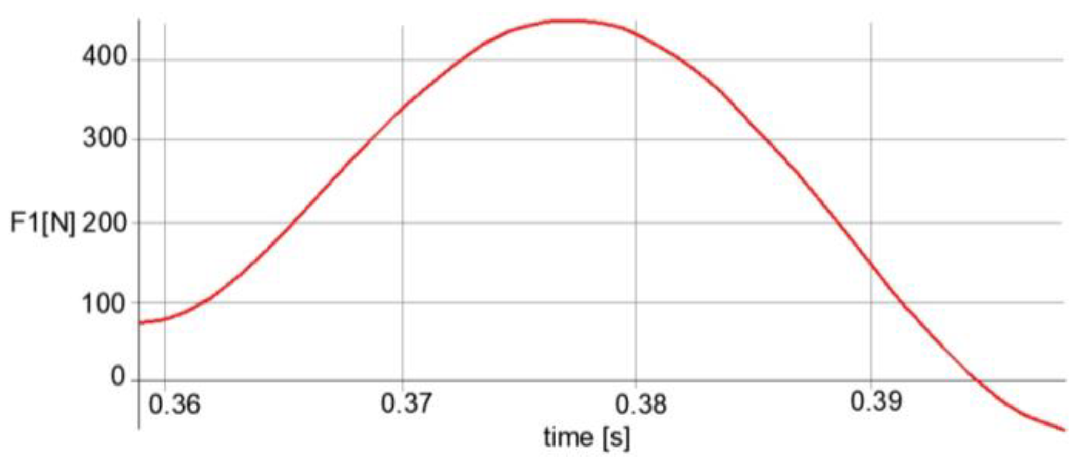
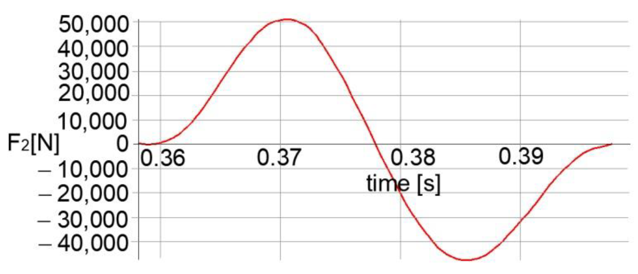
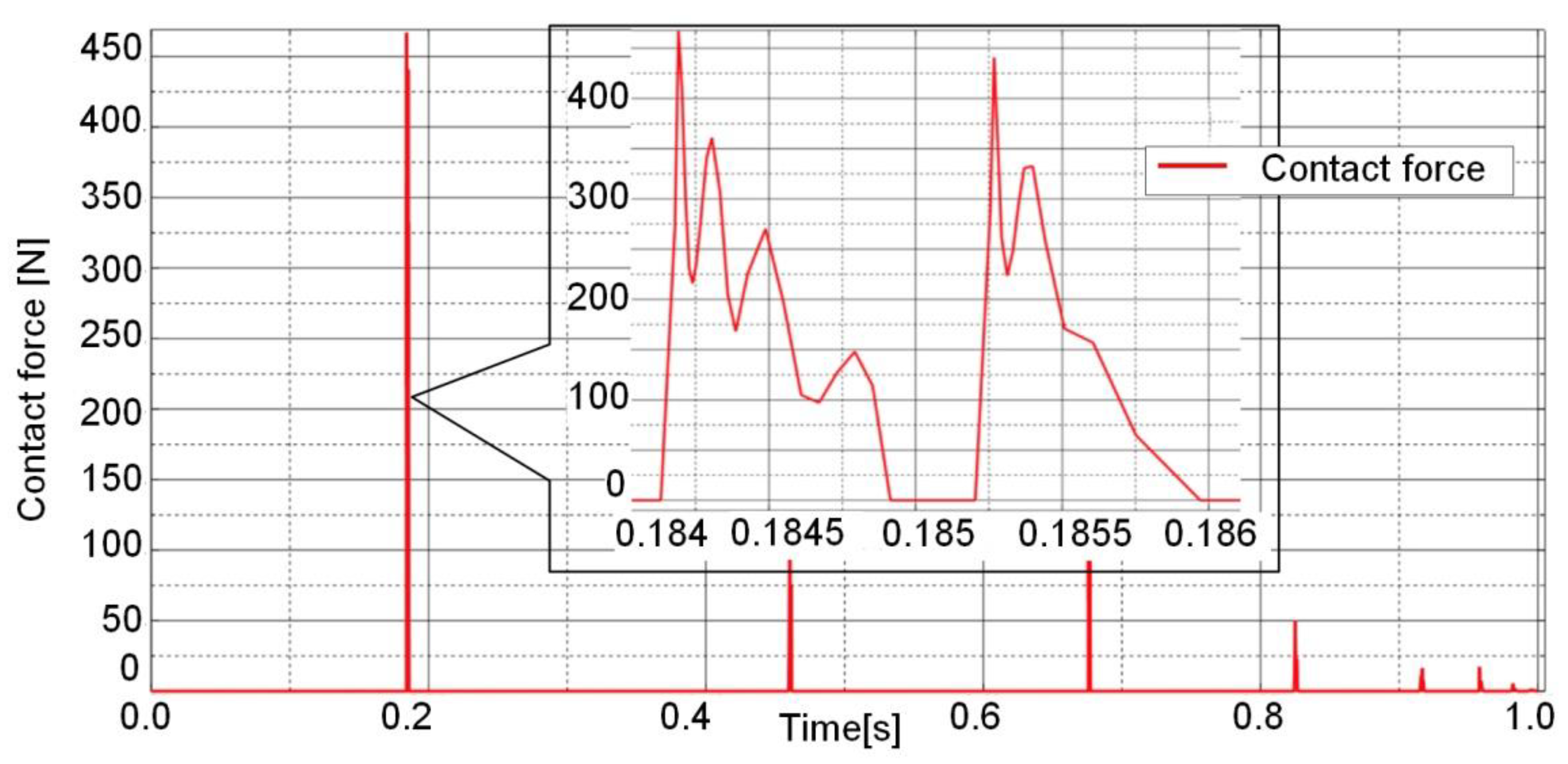
The impact between these components occurs at the time t = 0.1824 s. Thus, it can be observed that the displacement after impact shows a quasilinear variation until the time t = 0.2265 s, when the bar loses contact with the prismatic body component. At the impact moment the bar speed suddenly increases and it records a maximum value of 1325 mm/s. Accordingly, the impact force will occur at the contact moment and it records values ranging from zero to 205.5 N. Between the time interval of 0.1824—0.1862 s, the considered force will record many harmonics and one of them reaches a high value of 406.66 N as it can be seen in the detailed view in Figure 17. This variation has the following dynamic parameters values: k = 48,049, e = 2.2, c = 6, d = 0.01. In addition, this dynamic analysis was set up for an integration step equal to 1 × 10⁻⁴.
By comparing the variation diagrams in Figure 12 and Figure 16, it can be noted that for a high value of the damping coefficient, the number of harmonics will increase, whereas the transversal elastic displacement will decrease.
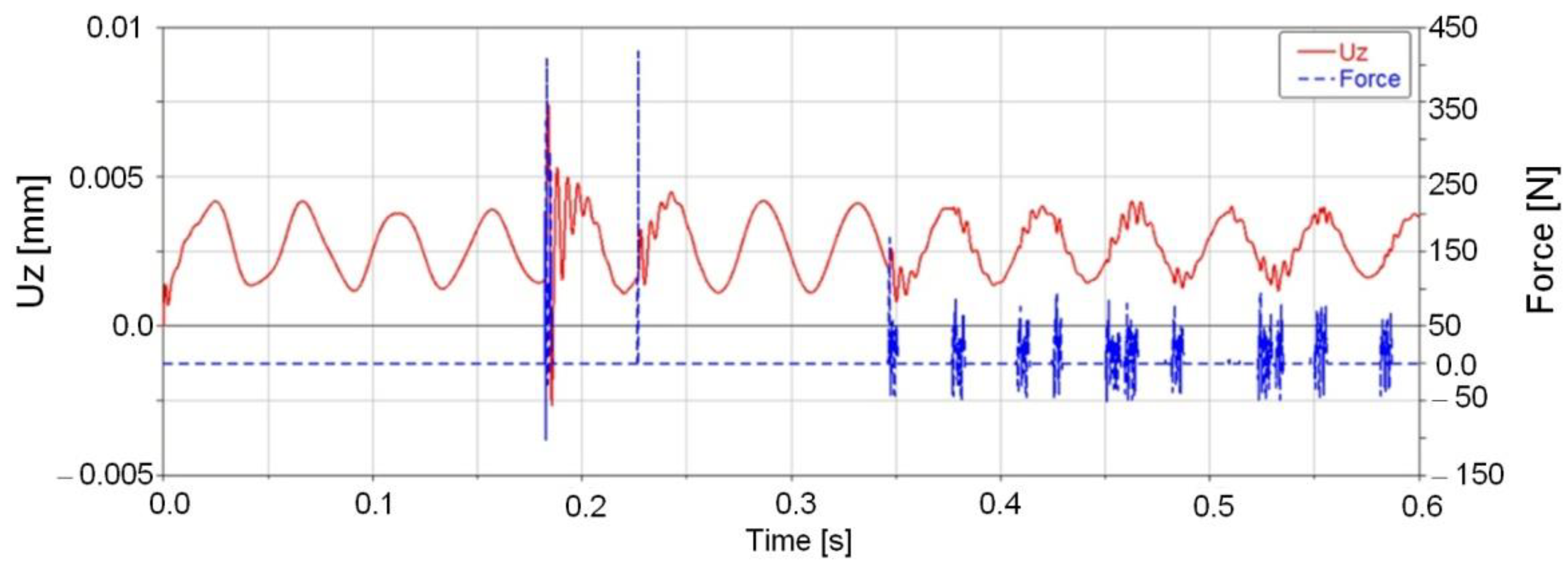
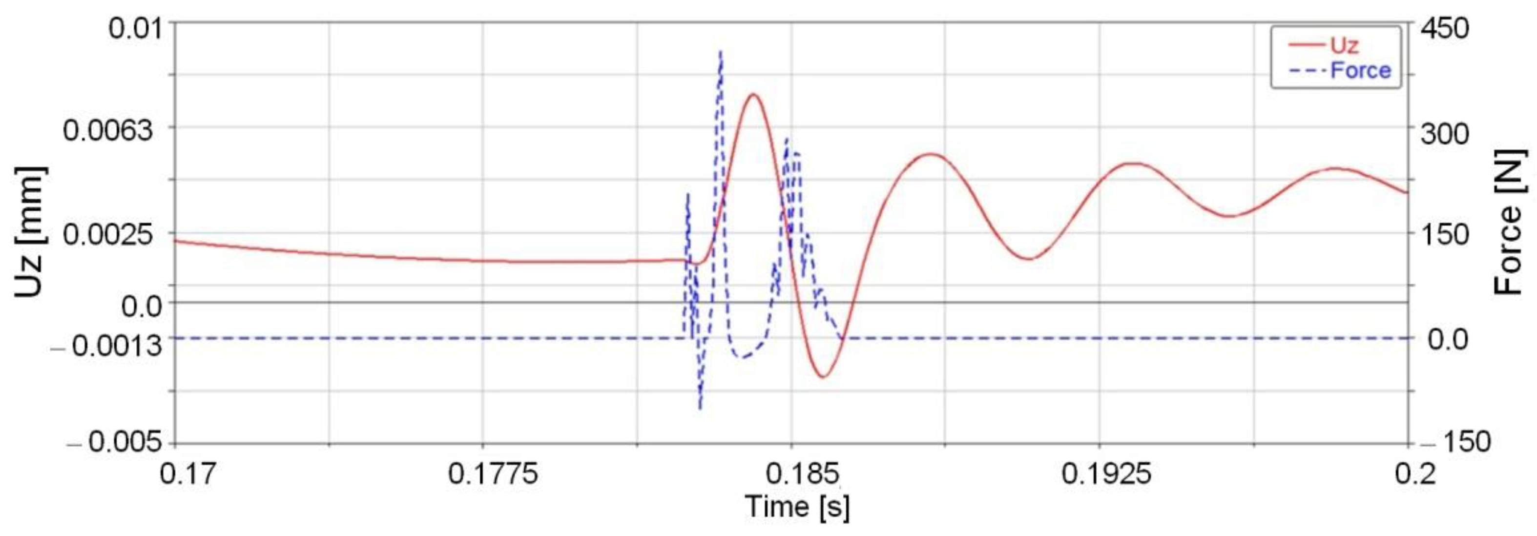
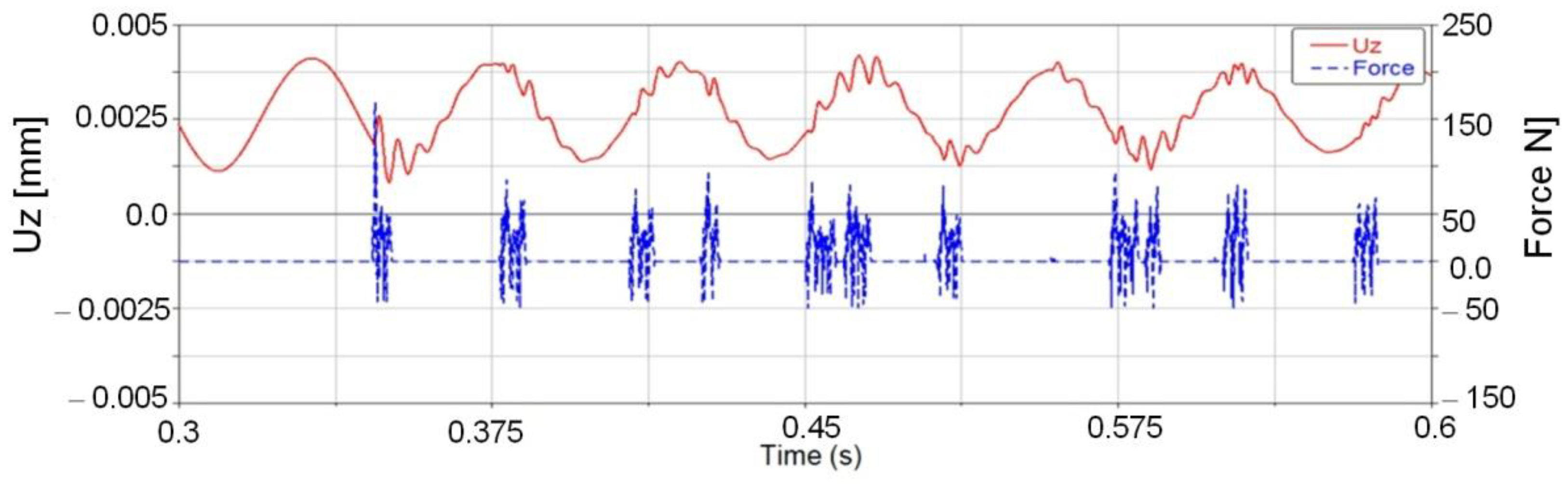
Figure 18 shows the force impact and transversal elastic displacement during time of the prismatic body component considered as a solid deformable one. These variations correspond to an impact force dynamic model where the damping coefficient is equal to c = 6. A detailed view of these variations is shown in Figure 19, which corresponds to the impact force and elastic displacement during the first impact. Another aspect is represented through the diagram in Figure 20, describing the entire impact force and elastic displacement variations on each impact between the bar and prismatic body components.
2.3. Impact Analysis with Finite Element Method
To analyze the impact phenomenon, based on the finite element method, three software programs were used, namely: Abaqus, ANSYS Workbench and ANSYS Mechanical APDL. For the impact phenomenon analysis with ANSYS the following steps were followed: the mechanical system CAD model was imported; the kinematic joints were defined; the entire model was meshed with proper finite elements and material and inertial properties were also defined; there were introduced the contour conditions and the contact between the bar and the prismatic body components was established when that had a free fall at the one end and touched the prismatic body.
The aim of this analysis regards the dynamic parameters, which define the contact between the bar and the prismatic body. Thus, many contact models, such as the ones below, were created:
(a) Frictionless contact, characterized by behavior-symmetric, stabilization damping factor-10, pinball radius—5 mm. In this case, the integration step was set up at 1 × 10⁻⁴ which corresponds to the hypothesis of large deflections. Time variation diagrams were identified for the following parameters: prismatic body stress, computed by considering a local coordinate system solitary with this component and dynamic parameters, which define the impact phenomenon between the bar and the prismatic body, namely, penetration depth, friction stress, contact pressure and contact force. For this model, the contact force is represented in Figure 21 and Figure 22.
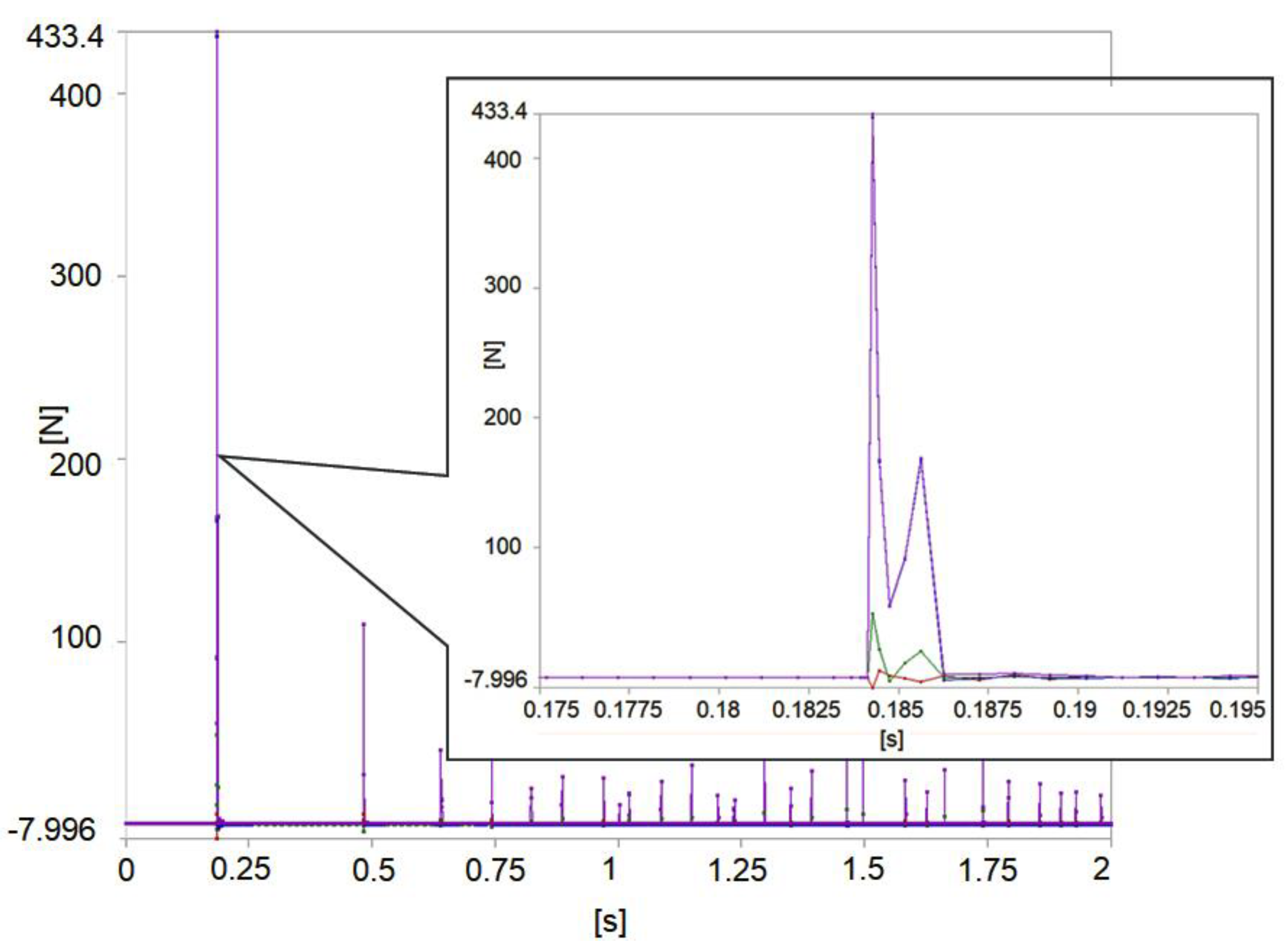
(b) Frictionless contact when the stabilization damping factor is equal to 0.1 and the integration step is equal to 1 × 10⁻⁴. With reference to the previous case, one it can note a decrease of amplitude for the resultant elastic displacement and an increased number of harmonics for all the monitored kinematic and dynamic parameters after the first impact. Thus, the contact force records a maximum value during the impact of 433. N and afterwards, the values will be small due to the damping phenomenon (Figure 23). Considering the diagrams reported in the first case (case a), it can be observed that after the impact, all the monitored parameters reach absolute values at the same time instants, whereas different variation forms are reported. By having in sight the fact that in all the modeling cases the bar motion in a free fall drop records high amplitudes, the finite element analysis was setup under the large deflections hypothesis. Thus the used finite elements support the contact modeling under this hypothesis. This setup was done in order to evaluate in a correct manner the bar component motion before and during the impact phenomenon.
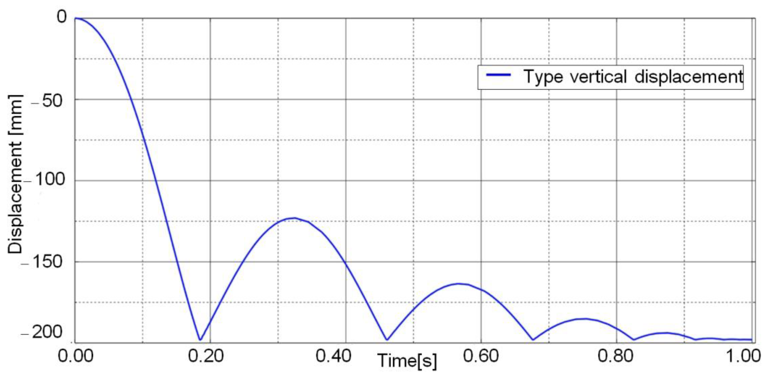
It can be observed that during the time interval 0 to 0.18517 s, the bar component will have a free motion under the gravity force until the impact momentum with the prismatic body component (this occurs at time = 0.18426 s). From the reported diagram it can be seen that the impact length period is around 0.002 s (between time = 0.18426–0.18626 s). After the impact, the displacement amplitude of the bar component will decrease due to the damping phenomenon, as it can be seen in Figure 24. The contact problem processing between the bar and prismatic body components take the time variations of the following parameters: contact pressure, sliding distance, friction stress, penetration and contact force.
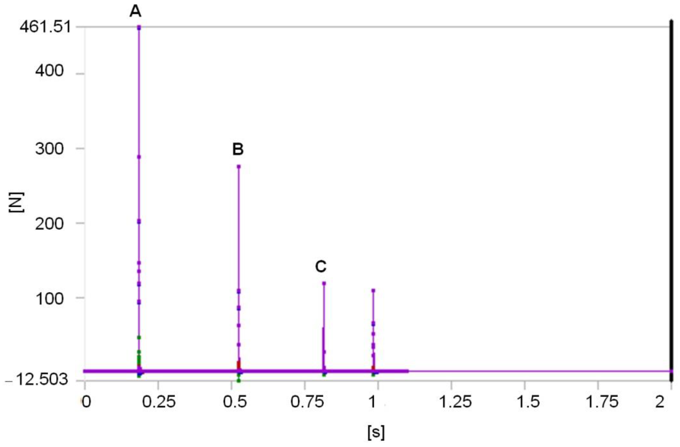
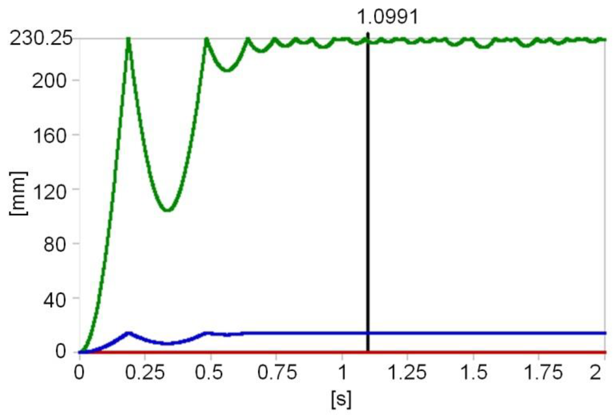
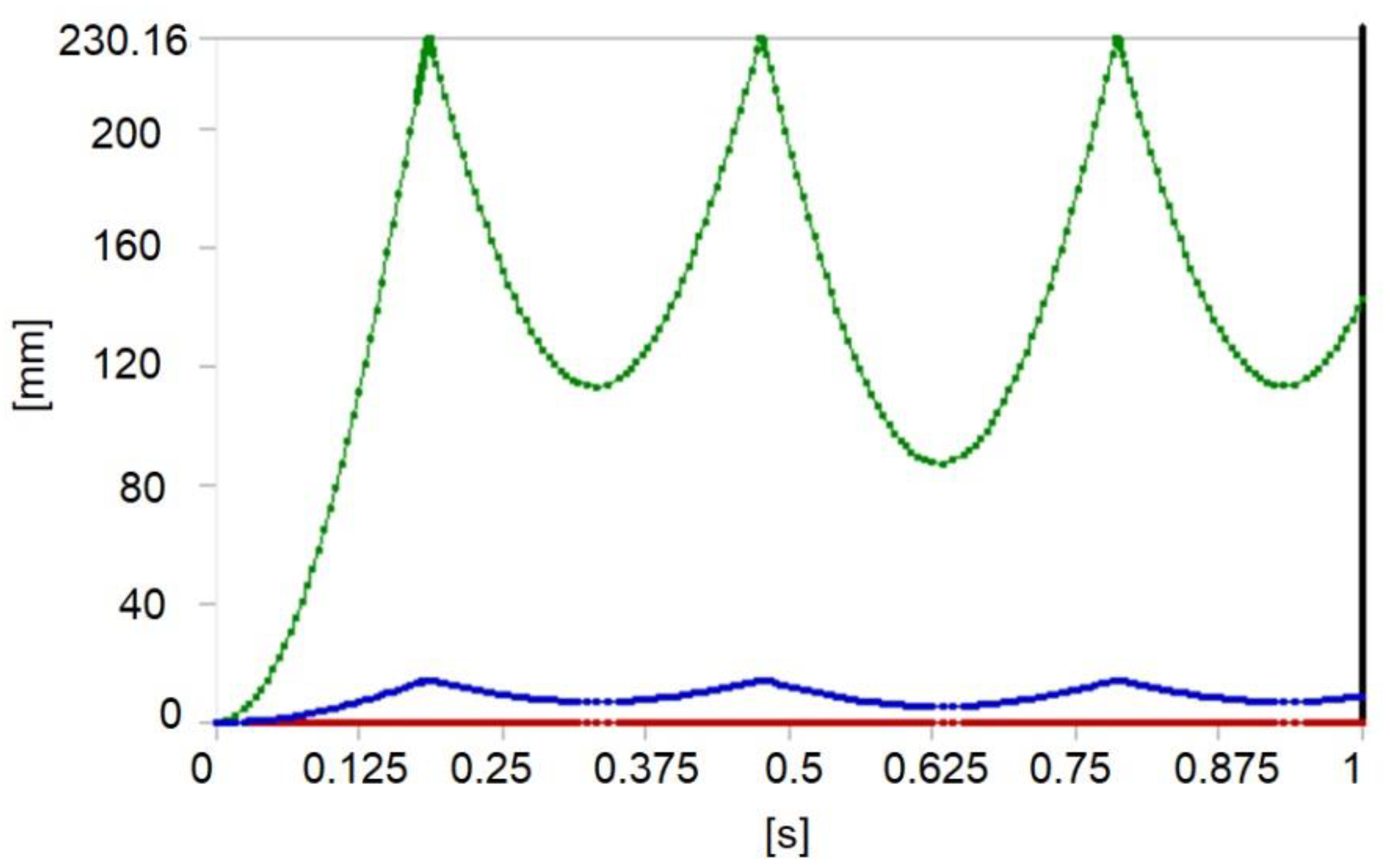
(c) Contact type rough, where the stabilization damping factor is equal to 6. For this contact type it was remarked that the impact force has a higher value, i.e., equal to 915 N. In addition, the bar motion amplitude after the first impact is higher than in the other cases. Thus, the impact was influenced by the quality of the contact surfaces. The obtained results are reported in Figure 25, Figure 26 and Figure 27.
In Figure 25 can be observed that the bar component displacement amplitudes will not decrease immediately after the impact time period. They reach high values around 230.16 mm. The reason for this behavior is represented by the base component surface, which is rough and the analyzed contact problem was included in this hypothesis of contact definition.
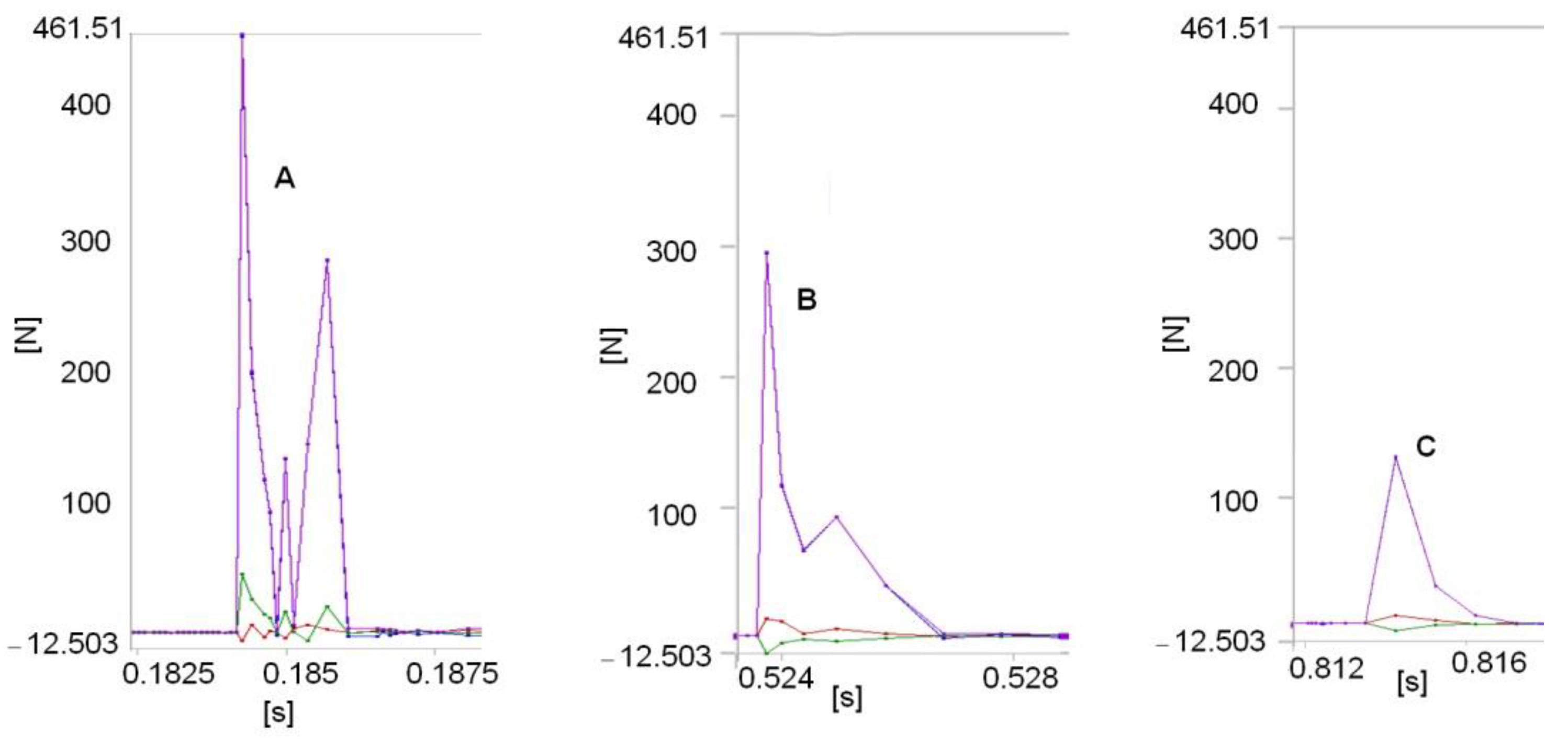
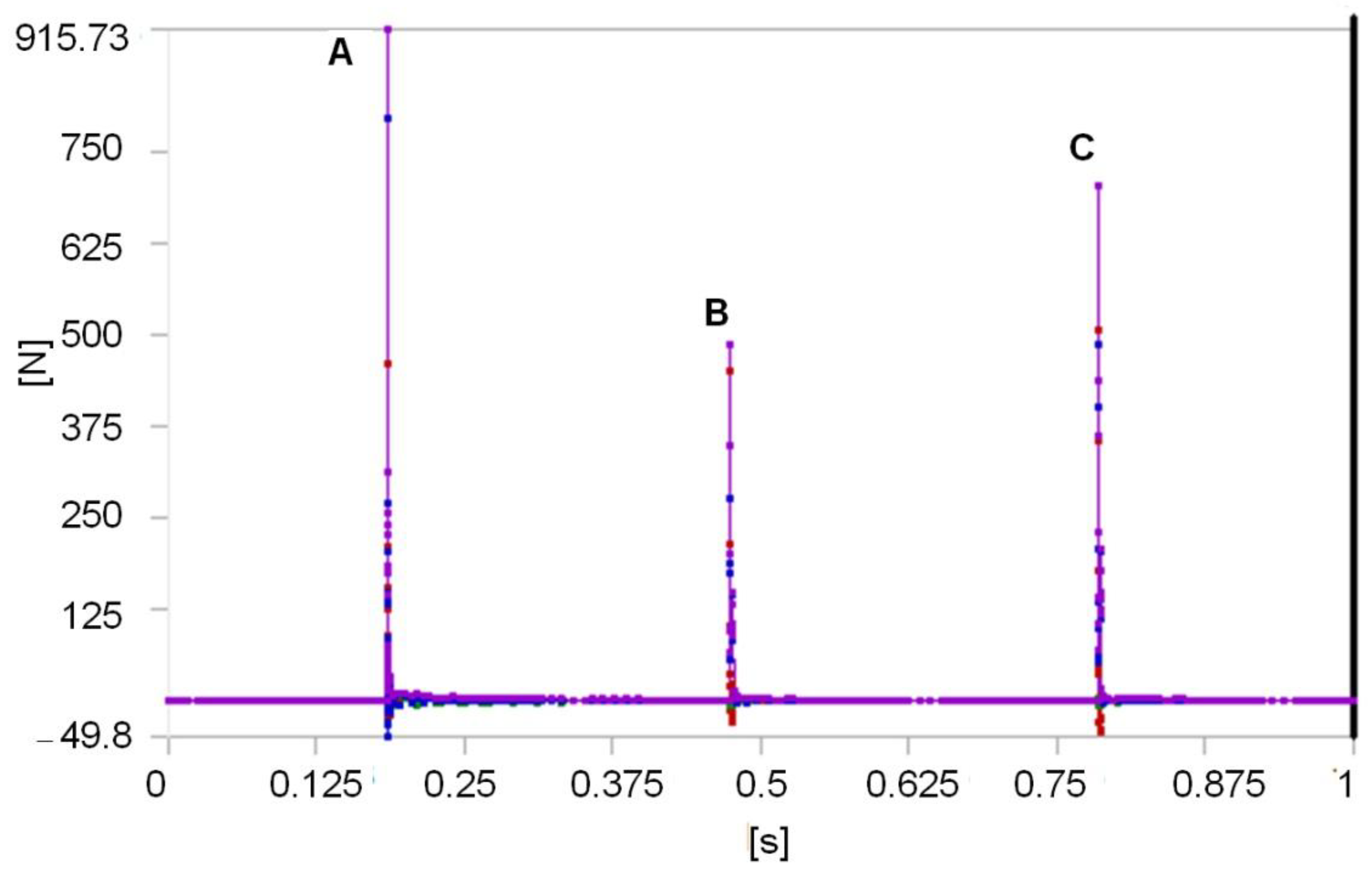
Thus, the impact force records high values at points A, B and C, as shown in Figure 26. A correspondence time interval between the bar component displacement variation and the force at the impact moment and after impact can be spotted.
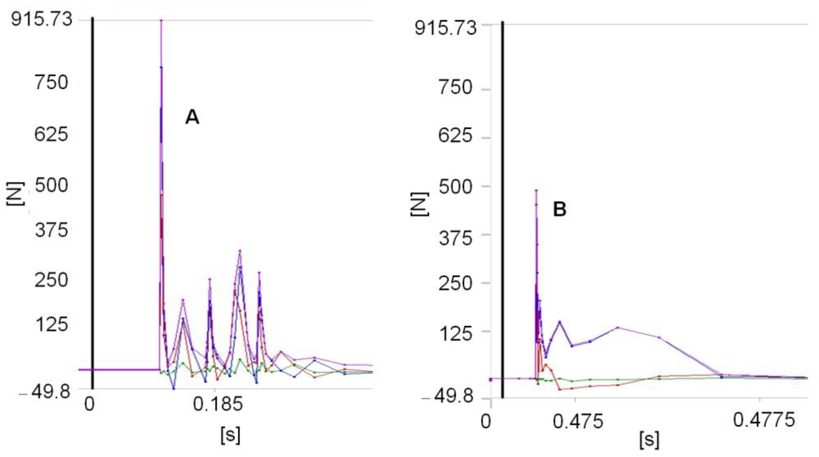
Figure 27 provides details of the impact force variation with time for the most important contact zones, namely, zone A and zone B. It can be remarked that the time period of the impact is higher than the other time periods. In addition, after the first contact, the time periods were smaller for zones B and C compared to Zone A. High values were recorded for the first contact, namely, 915.73 N (corresponding to zone A), then they decreased to around 515 N (corresponding to Zone B) and to around 735 N (corresponding to Zone C).
2.4. Impact Modeling with Abaqus
In order to study the impact phenomenon under the Abaqus software environment, the same mechanical system model that was presented in Figure 11 was considered. The virtual prototyping accomplished with the Abaqus software underpins a kinematic model made up of five parts connected together through kinematic joints. There was made a similar setup as in the previous case studies and the main objective was to determine the impact force variation and the elastic displacement during the impact phenomenon. Thus, the obtained results are reported in Figure 28 and Figure 29.
Figure 28 presents the contact force variation during time at the impact moment and after, between the bar and the prismatic body component. This reaches a maximum value of 450 N. In Figure 29, the bar component displacement in a free fall, before and at the impact moment, records values within an amplitude of 200 mm, which will decrease after the first impact.
3. Dynamic Analysis of the Impact in the Case of a Crank-Connecting Rod Mechanism
With the Adams program, a connecting rod-crank mechanism is examined. Due to the modeling of a radial clearance in the rotational joint between the connecting rod and the slide, an impact occurs, which generates a force impacting the dynamics of the mechanism. The radial clearance resultant value in the rotational joint is equal to 1.1 mm. A procedure was designed for generating the torque, under the Adams programming environment, to actuate the entire mechanism in the impact force conditions between the connecting rod and the slide. The following steps are required to create the impact function:
- time variation functions are defined for the interest marker displacement and velocity (the marker that materializes the force point application, i.e., marker 13, placed in the joint rotation center);
- the impact function will be created based on the following kinematic and dynamic parameters: displacement, dy_ MARKER_i, velocity, vy_ MARKER_i, for marker i, stiffness k, exponential coefficient e, damping c, penetration d, as follows:
IMPACT (.MODEL_1.dy_ MARKER_i, .MODEL_1.vy_ MARKER_i, k, e, c, d)
One will examine the impact force effect developed at the connecting rod-slide contact on the evolution of the mechanism kinematic parameters, in two cases, a mechanism with rigid elements and a mechanism with deformable elements, respectively.
3.1. Impact Dynamic Analysis with Rigid Elements
A function is defined in order to identify the motor torque, based on the following expression:
where: Mm represents the engine torque (Tm—reported in diagrams); M0 is the initial torque; ω0 is an initial angular velocity; WZ represents the resulting angular velocity during the engine torque.
There are three markers placed in the center of rotation of the crank, namely, MARKER_1, MARKER _9, MARKER 10. These will materialize the origins of three reference systems (two reference systems that define the rotation torque and one mobile integrated with the crank). The mechanism dynamics was studied for the dynamic parameters with several sets of values in the impact force structure. These are represented through diagrams as seen in Figure 30, Figure 31, Figure 32 and Figure 33.
The functions used for processing the diagrams in Figure 30 are:
Torque:(−10,000,000 * (1 − WZ(MARKER_1,MARKER_9,MARKER_10)/10);
IMPACT(.MODEL_1.dy_13, .MODEL_1.vy_13, 0.0, 10,000, 0.1, 10, 1 × 10⁻³)
The functions that were the basis for processing the diagrams in Figure 31, Figure 32 and Figure 33, are:
Torque: (−10,000,000 * (1 − WZ(MARKER_1, MARKER_9, MARKER_10)/10)
IMPACT(.MODEL_1.dy_13, .MODEL_1.vy_13, 0.0, 10,000, 0.01, 10, 1 × 10⁻³)
The reported results in Figure 33 generate the following functions:
Torque: (−10,000,000 * (1 − WZ(MARKER_1, MARKER_9, MARKER_10)/10)
IMPACT(.MODEL_1.dy_13, .MODEL_1.vy_13, 0.0, 10,000, 0.2, 10, 1 × 10⁻³)
Torque: (−100,000,000 * (1 − WZ(MARKER_1, MARKER_9, MARKER_10)/10)
IMPACT(.MODEL_1.dy_13, .MODEL_1.vy_13, 0.0, 100,000, 0.2, 10, 1 × 10⁻³)
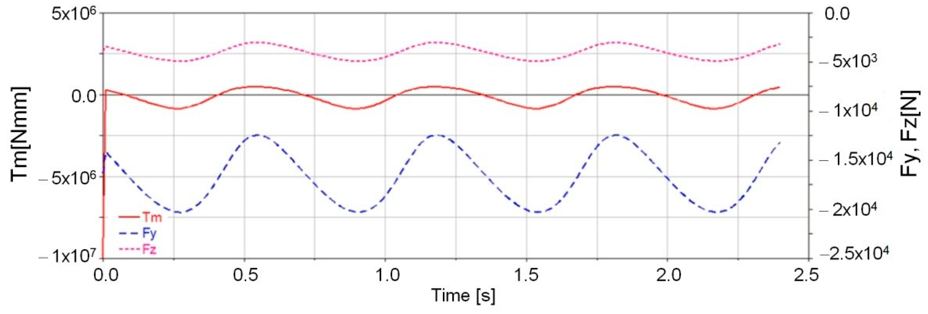
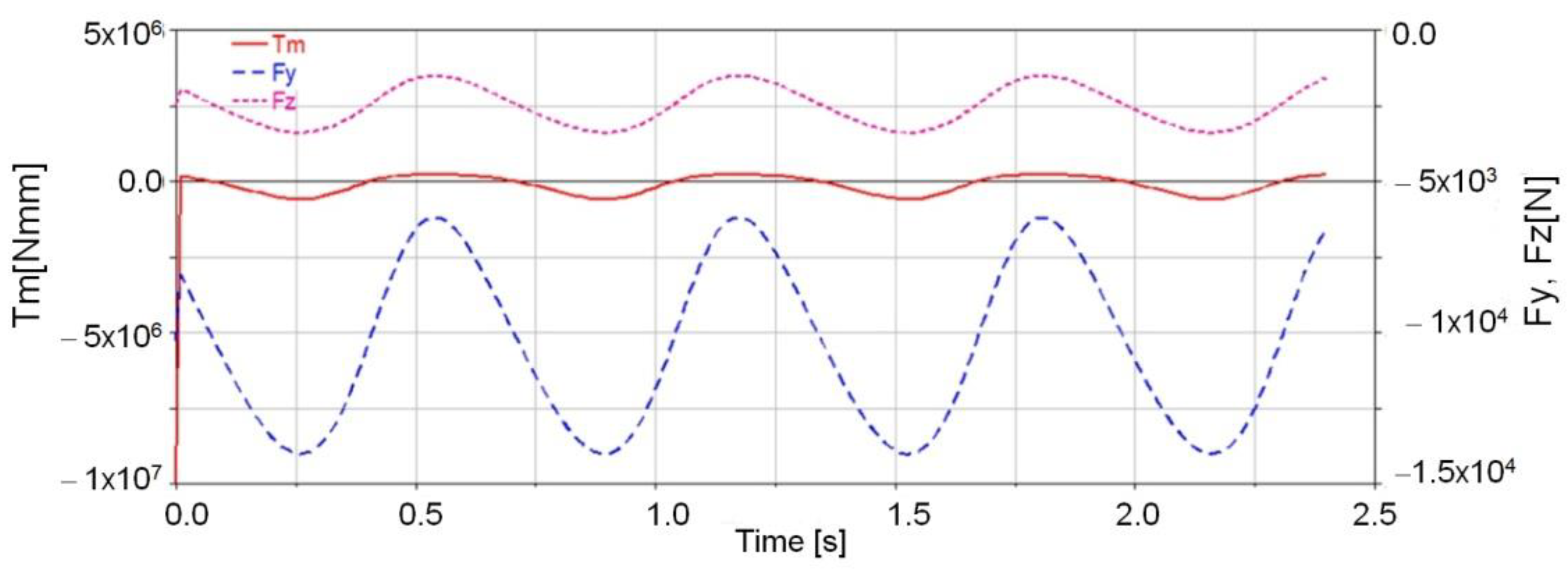
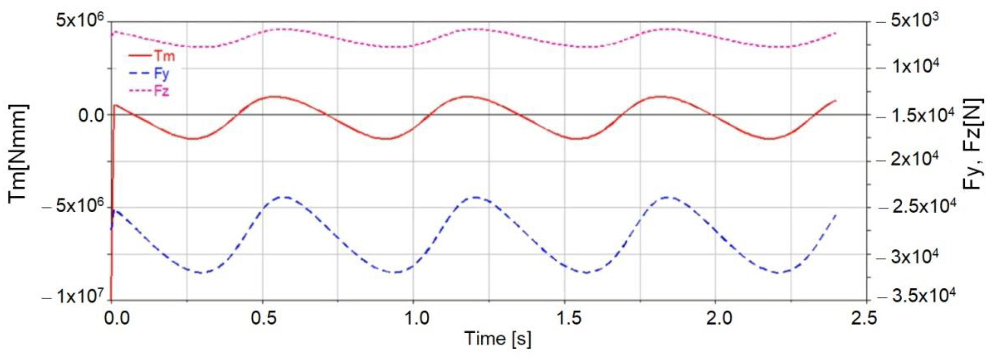
Figure 30, Figure 31, Figure 32 and Figure 33 show the time variation diagrams for the engine torque and the two components of the impact force along the y and z axes.
Figure 30 indicates that the three components have a cyclic variation, and that each cycle was repeated at an interval of 0.63 s.
The engine torque in each case reaches a maximum value at the start-up, due to the mechanism inertia in the first milliseconds. In addition, as seen in Figure 30, the engine torque maximum value on each cycle is around 4.09 × 10⁵ Nmm and the minimum value around −8.25 × 10⁵ Nmm.
It was found that the component along the y-axis of the force reaches higher values than the one along the z-axis. Thus, the component along the y-axis has a maximum value of 12.375 N, and the one along the z-axis has a maximum value of 3.500 N.
In Figure 31 the impact force components have the same variation shape as the ones in Figure 30, with the specification that the extreme values are lower given the dynamic parameters, except for the force exponent which was smaller in this case. The component along the y axis reaches a maximum value of 6181.81 N and around 1462.5 N along the z axis.
In Figure 32, the engine torque and the impact force dynamic parameters are kept, except for the force exponent, which increased. This led to a significant increase of the two force components extreme values along the y and z axes, i.e., 23,875 N for the y-axis and 5.750 N for the z-axis.
In Figure 33 the structure stiffness in the case of the impact force changes, consequently, a higher value of the initial moment M0 is required. In this case, the maximum and minimum values of the engine torque and the impact forces components change, resulting in 8.63 × 10⁶ Nmm for the engine torque, the value of the component along the y-axis being around 2.7 × 10⁵ N and the value of the component along the z axis being of 64,925 N.
As a remark, due to the eccentricity of the spindle-bearing coupling type, the two dynamic components (engine torque and impact force), record jumps in an infinitesimal time at the mechanism start-up. We will consider that these jumps can be neglected and find that the mechanism has a correct cyclic operation, even if in some cases the extreme values of the dynamic components are high. For this reason, a dynamic study of the mechanism is required, regarding the elements in contact as deformable.
3.2. Impact Dynamic Analysis with Deformable Elements
3.2.1. Mathematical Considerations
A geometrical modeling of the engine mechanism was performed using the SolidWorks software, according to its dimensions and construction geometry.
The mechanism modal dynamic analysis was performed via the ADAMS program and it involved two important steps:
- Evaluating the natural frequencies and vibration modes;
- Elastic dynamic analysis.
The modal analysis mathematical models of a mobile mechanical system with deformable elements were proposed and developed by Craig and Bampton [23].
Thus, the equations defining the flexible body motion are differentiated from Lagrange’s equations [23]:
where: L is the Lagrange defined as: L = T − V; T and V are the kinetic energy and potential energy, respectively, F is the energy dissipation function; Ψ are the constraint equations; λ are the constraints Lagrange multipliers; ξ are the generalized coordinates; Q are the generalized applied forces (the applied forces projected on ξ).
The flexible body generalized coordinates are:
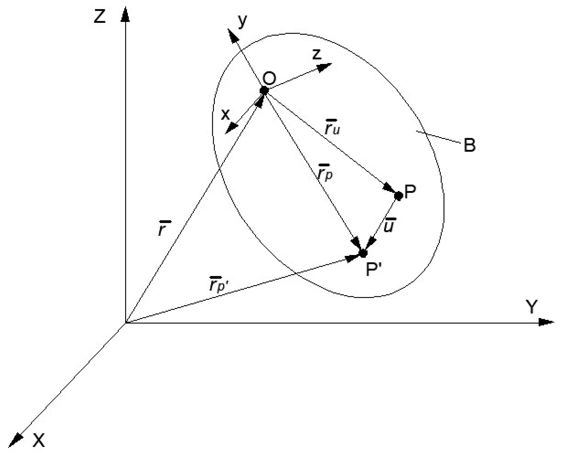
The instantaneous position of a point attached to a node on a flexible body, according to Figure 34, is given by the following mathematical expression:
where: is the position vector from the fixed (ground) reference system origin to point O where the local reference system origin is located of the flexible body; is the position vector of the undeformed position of point P, according to the local reference system attached to body B; —the translational deformation vector of point P, the position vector of the body un-deformed position to its deformed position.
The elements of the vector , x, y and z are the flexible body generalized coordinates. The orientation is evaluated and characterized by the Euler angles set, Ψ, θ and ϕ, according with Figure 34.
The translational deformation vector is a modal superposition as follows:
where: Φp is the part from the modal matrix corresponding to the node P translational degrees of freedom.
The Φp matrix dimension is 3 × M, where M represents the number of vibration modes. The modal coordinates qi, (i = 1, …, M) are the flexible body generalized coordinates. The angular deformations vector was obtained in a similar mode as the translation deformation vector, using a modal superposition, similar to the following expression:
where Φ*p is the modal matrix part corresponding to the rotational degrees of freedom of node P. The Φ* matrix dimension is 3XM, where M is the number of modes of vibration [18].
3.2.2. Numerical Simulation
The same planar mechanism as the one with the rigid elements will be analyzed, but in this case, the connecting rod is considered as a deformable element. The connecting rod transformation from a rigid body to a deformable body was based on the finite element method, adopting the following procedure: The connecting rod body is meshed in tetrahedral finite elements, with a finer network in the joints contact areas.
The flexible body, obtained through the mesh network, must have its attachment points corresponding to the kinematic joints. The connection is made through nodes, with a spider type network. The analytical model of the engine torque is the same as Equation (25) namely ω0 = 10 rad/s, M0 = −100,000 Nmm.
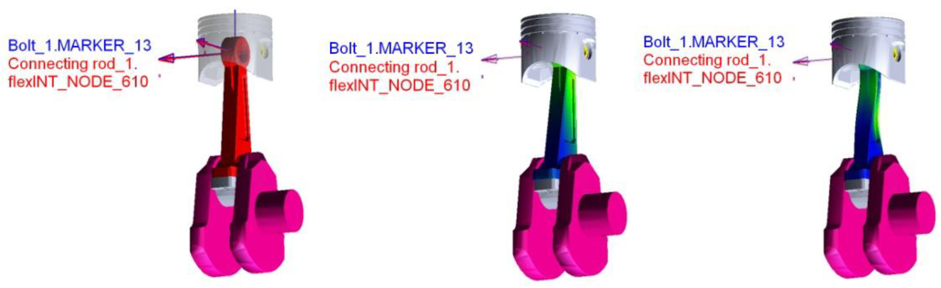
Thus, the time variation laws for the mechanism kinematic and dynamic parameters for two operating cycles are identified. Some snapshots during this simulation are shown in Figure 35.
Figure 35 indicates the location of one node in the center of the bolt as a revolute joint between bolt and connecting rod head. This node is part of the network of hexahedral finite elements in which the mechanism connecting rod is meshed (node 610).
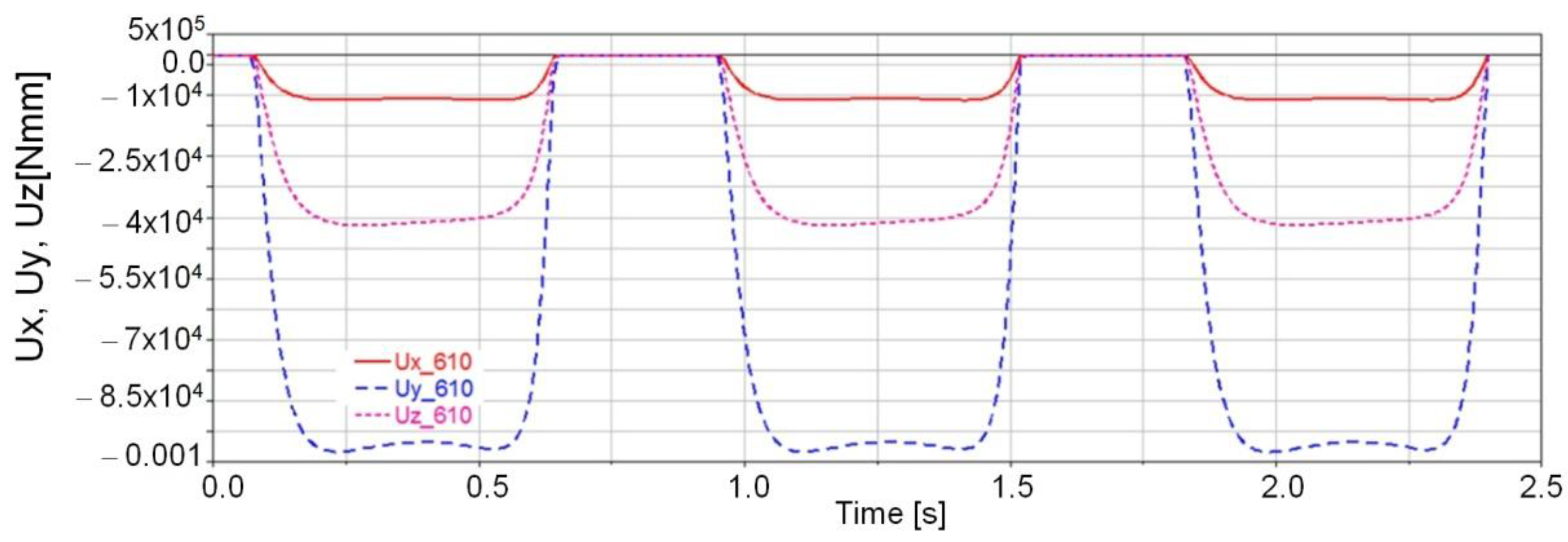
The time variation laws are identified for the kinematic parameters that define the motion of the node 610, i.e., the translational displacement along the x and y axes. These are reported in Figure 36 and Figure 37 in case of the deformable body movement.
The impact structure function is defined as: IMPACT(.MODEL_1.dy_flex13, .MODEL_1.vy_flex13, 0.0, 20,000, 0.1, 10, 1 × 10⁻³), with the following values of the dynamic parameters: k = 20,000, e = 0.1, c = 10, d = 10−3.
In addition, as seen in Figure 35, the connecting rod deformed shape for vibration mode no. 3 with a natural frequency records a value of 6.515 × 10⁴ Hz and for vibration mode no.10 with a natural frequency of 1.061 × 10⁴ Hz.
The performed dynamic analysis consists of two major stages:
- modal-dynamic analysis with calculating the engine torque for the mechanism actuation;
- kinematic and dynamic parameters analysis of the generated contact during the impact between the bolt and the connecting rod head.
The modal-dynamic analysis presupposes the natural frequencies evaluation and the component proper vibration modes when this is considered deformable one.
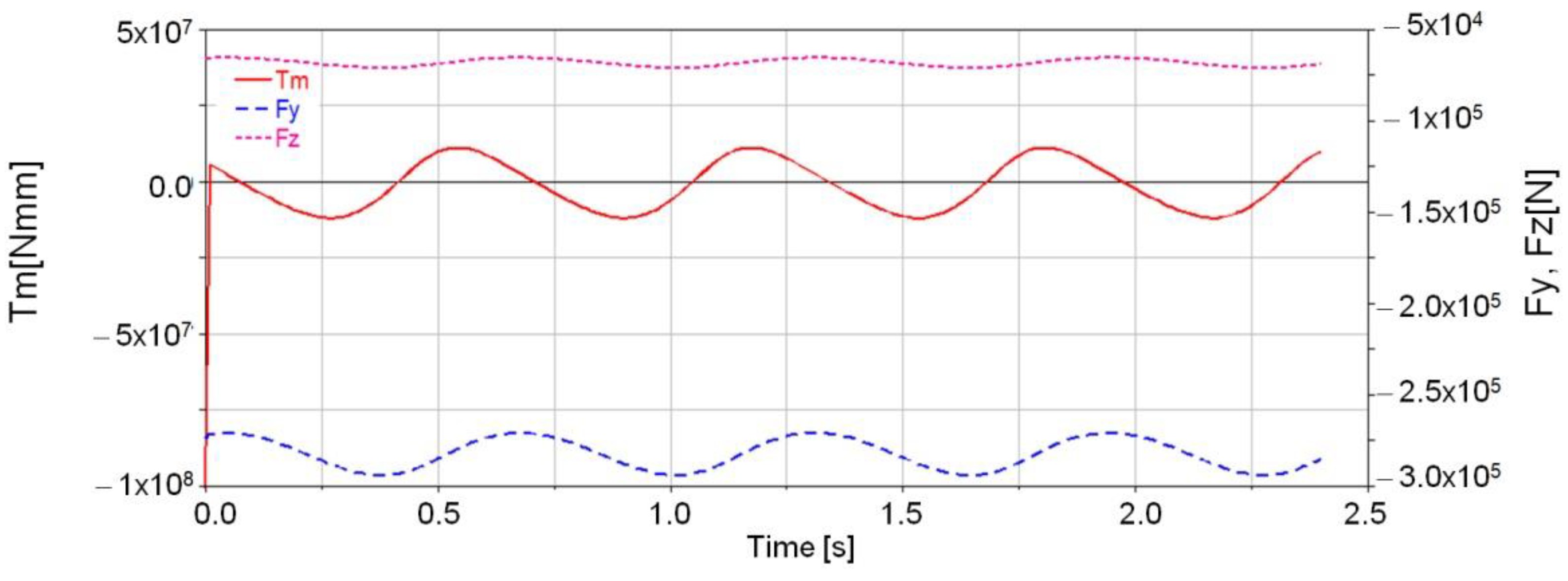
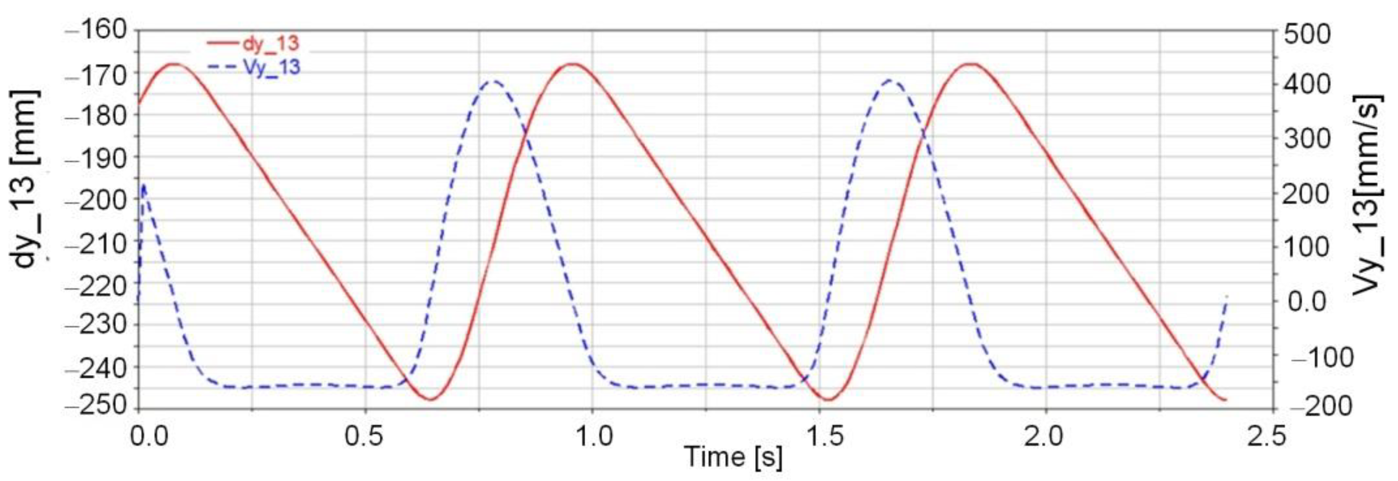
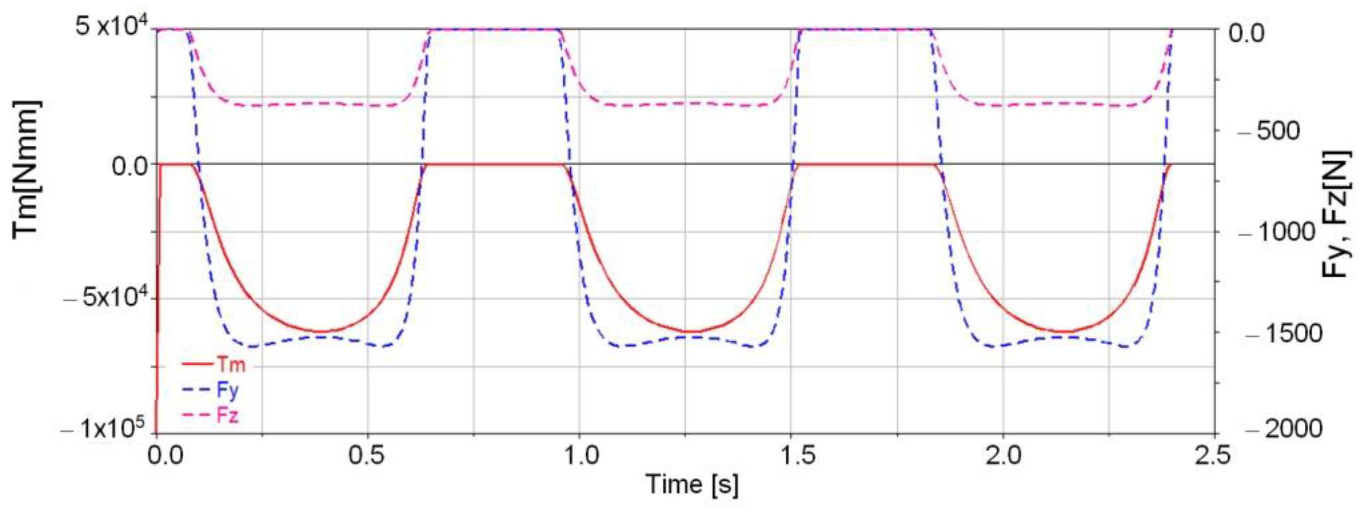
The kinematic parameters involved in the impact force dynamic model definition are the displacement and velocity of the marker 13. This marker is identified as the position with the node 610, so it is located in the bolt center of the revolute joint (between the bolt and the connecting rod). Figure 38 shows the displacement and velocity time variation for marker 13 along the y-axis. Based on Equation (25) and on the numerical simulation performed with the Adams program, the engine torque variation diagram reported in Figure 39 was obtained. In Figure 39 is observed that the engine torque has a periodic variation, with the maximum amplitude around 50,000 Nmm. The jump recorded at start-up results from existence of the impact generated by the shock in the joint.
Figure 39 presents the behavior mode of the impact force on two elements brought in contact, i.e., the connecting rod and the bolt. It is important to note that the effect of this force is visible mainly in the area of maximum eccentricity between the connecting rod and the slide. Figure 39 it shows the time variation diagrams for the considered components along the y and z axes of the impact force. Thus, the engine torque variation mode is close to the impact force variation mode.
4. Results and Conclusions
The impact phenomenon was examined in two major cases, namely the impact resulting from the contact between the two bodies, when one of them was fixed and the other one was mobile, actuating freely under gravity and the impact generated by two mobile bodies from a multi-body mechanical system structure.
In the first case the impact analysis was done through an analytical method and virtual prototyping with the Adams, ANSYS and Abaqus software. Thus, the following conclusions were drawn:
- The mathematical model corresponding to Equation (16) is compatible with the Adams software theory, in relation to the impact phenomenon analysis. A Maple program sequence was derived, which can be numerically processed based on the created mathematical models by considering two major impact force components, namely, the stiffness component and the viscous component. These component variations with time were presented in Figure 7 and Figure 8.
- The dynamic parameters were processed via the Maple program by considering Equation (16) with the numerical values indicated in Figure 7 and these corresponds to the virtual models obtained with the Adams software (Figure 16 and Figure 17), with Ansys software (Figure 24) and Abaqus software (Figure 28), respectively.
- For the analytical models and numerical processing of the imported models with the Adams software, the bar component motion was monitored in a time interval equal to 0.6 s.
- By modifying the damping coefficient value to c = 6, it can be remarked that the impact force maximum value will be modified, as well, along the number of contacts between the bar component and the prismatic body. At the same damping coefficient, by keeping the contact conditions and the integration step of the equations system, which dictate the bar component motion, one can see that the impact force values are not compatible with these cases, namely, analytical case (Figure 9), numerical simulation with the Adams software (Figure 16) and the finite element analysis (Figure 24 and Figure 28).
Thus, the impact analysis based on the finite element method for the proposed model was performed for several cases: contact without friction, contact with friction and a rough type contact. The following kinematic and dynamic parameters were considered: the bar component displacement on three time intervals, i.e., before the impact, during the impact and after the impact, depth penetration; sliding distance, contact pressure and contact force.
Based on these parameters, the analysis was performed for different damping coefficient values and the same materials for contact analysis. In addition, the same integration step for differential equations was preserved. Thus, it was concluded that the variation forms of the impact force are the same for each analyzed case (Figure 22, Figure 24, Figure 27 and Figure 28).
The displacement bar component amplitude is different in terms of value and frequency, depending on the contact and damping coefficient values during motion (Figure 23, Figure 25 and Figure 30).
A parameter which one can consider very important is represented by the prismatic body’s elastic displacement variation due to the impact between the bar component and the prismatic body. These variation diagrams are represented and analyzed in Figure 13, Figure 14 and Figure 15 (via the Adams software). These are very important because they can be compared relatively easy to the ones which were further obtained through experimental analysis.
A crank connecting the rod mechanism was examined, in which a radial clearance was considered in the joint that connects the connecting rod and the piston. Under these conditions, during the engine mechanism operation, a developed impact has major influence on the kinematic parameters that define the movement of the considered bodies brought in contact (the connecting rod and the piston). The dynamics of the mechanism involved two cases, namely, when the kinematic elements are rigid bodies and the case when the connecting rod and the piston are deformable ones.
The impact force dynamic model in the two cases was built on the following parameters: stiffness, force exponent, damping and penetration depth. These parameters were determined by several sets of numerical simulations that were based on the interface between the variation of the impact force and the variation of the engine torque, in the conditions of a cyclic operation of the mechanism. It was found that the results of the numerical simulation, mainly the impact force and the engine torque, are compatible with the mechanism cyclic operation if the elements deformability is taken into account, as well.
Variations of the kinematic parameters were reported, especially in the contact area of the connecting rod-piston, by monitoring the nodes movement on the joint finite elements.
As it was mentioned before, the impact dynamics was analyzed for two cases. Thus, in the first case the impact dynamics between two distinctive bodies were analyzed with the use of the finite element method. This allowed us to determine the kinematic and dynamic factors’ influence mode on the impact force size and variation mode. Moreover the friction coefficient influence through contact surface quality and damping factor can be remarked. Thus, multiple tests were performed with different material types, different friction coefficients which were associated with damping factor values sets. By considering these tests, an influence rapport of the mentioned factors which depends with the contact body stiffness respectively impact force amplitude and frequency during and after impact phenomenon was established.
The obtained diagrams through impact phenomenon analysis in the second case show that impact force characteristics such as the amplitude and variation mode were influenced by assembly errors and kinematic parameters variation during motion. By having in sight other results from specific literature like [14], the impact force influence on mechanism torque was analyzed. Thus, the mechanism torque was established through a function definition under the MSC Adams environment. This function allows the user to perform a complete dynamic analysis of the combustion engine mechanism. In addition, the impact function presence which affects the engine mechanism functionality especially when this mechanism starts and the mechanism torque records high values can be observed.
Author Contributions
Conceptualization, S.D.; methodology, N.D.; software, S.D.; validation, N.D., S.D. and C.C.; formal analysis, A.C.; investigation, A.C.; resources, S.D.; data curation, A.C.; writ-ing—original draft preparation, S.D.; writing—review and editing, C.C.; visualization, S.D., C.C. and N.D; supervision, N.D.; project administration, S.D., C.C. and N.D.; funding acquisition, S.D., C.C. and N.D. All authors have read and agreed to the published version of the manuscript.
Funding
This research received no external funding.
Institutional Review Board Statement
Not applicable.
Informed Consent Statement
Not applicable.
Data Availability Statement
Not applicable.
Conflicts of Interest
The authors declare no conflict of interest.
References
- Ambrósio, J.A.C. Impact of rigid and flexible multibody systems deformation description and contact models. In Virtual Nonlinear Multibody Systems; Springer: Dordrecht, The Netherlands, 2003; pp. 57–81. [Google Scholar]
- Khulief, Y.A.; Haug, E.J.; Shabana, A.A. Dynamic Analysis of Large Scale Mechanical Systems with Intermittent Motion; Technnical Report No. 83-10; University of Iowa, College of Engineering: Iowa City, IA, USA, 1983. [Google Scholar]
- Hunt, K.H.; Grossley, F.R.E. Coefficient of Restitution Interpreted as Damping in Vibroimpact. ASME J. Appl. Mech. 1975, 42, 440–445. [Google Scholar] [CrossRef]
- Ahmed, S.; Lankarani, H.M.; Pereira, M.F.O.S. Frictional impact analysis in open-loop multibody mechanical systems. J. Mech. Des. 1999, 121, 119–127. [Google Scholar] [CrossRef]
- McCoy, M.l.; Lankarani, H.; Moradi, R. Use of simple finite elements for mechanical systems impact analysis based on stereomechanics, stress wave propagation, and energy method approaches. J. Mech. Sci. Technol. 2011, 25, 783–795. [Google Scholar] [CrossRef]
- Tempelman, E.; Dwaikat, M.M.S.; Spitás, C. Experimental and Analytical Study of Free-Fall Drop Impact. Testing of Portable Products. Exp. Mech. 2012, 52, 1385–1395. [Google Scholar] [CrossRef] [Green Version]
- Kantar, E.; Erdem, R.; Ozgur, A. Nonlinear Finite Element Analysis of Impact Behavior of Concrete Beam. Math. Comput. Appl. 2011, 16, 183–193. [Google Scholar] [CrossRef] [Green Version]
- Chen, C.-R.; Wu, C.-H.; Lee, H.-T. Determination of Optimal Drop Height in Free-Fall Shock Test Using Regression Analysis and Back-Propagation Neural Network. Shock Vib. J. 2014. [Google Scholar] [CrossRef] [Green Version]
- Corbin, N.A.; Hanna, J.A.; Royston, W.R.; Warner, R.B. Impact-induced acceleration by obstacles. New J. Phys. 2018, 20, 1–8. [Google Scholar] [CrossRef]
- Brun, P.-T.; Audoly, B.; Goriely, A.; Vella, D. The surprising dynamics of a chain on a pulley: Lift off and snapping. Proc. R. Soc. A Math. Phys. Eng. Sci. 2016, 472, 20160187. [Google Scholar] [CrossRef] [PubMed]
- Dankowicz, H.; Fotsch, E. On the analysis of chatter in mechanical systems with impacts. Procedia IUTAM 2017, 20, 18–25. [Google Scholar] [CrossRef]
- King, H.; White, R.; Maxwell, I.; Menon, N. Inelastic impact of a sphere on a massive plane: Nonmonotonic velocity dependence of the restitution coefficient. Europhys. Lett. 2011, 93, 14002. [Google Scholar] [CrossRef]
- Muller, P.; Heckel, M.; Sack, A.; Poschel, T. Complex velocity dependence of the coefficient of restitution of a bouncing ball. Phys. Rev. Lett. 2013, 110, 254301. [Google Scholar] [CrossRef] [PubMed] [Green Version]
- Yan, M.; Wang, T. Finite Element Analysis of Cylinder Piston Impact Based on ANSYS/LS-DYNA. In Proceedings of the 2012 International Conference on Mechanical Engineering and Material Science (MEMS 2012), Hong Kong, China, 27–28 July 2012. [Google Scholar]
- Žmindák, M.; Pelagić, Z.; Pastorek, P.; Močilan, M.; Vybošťok, M. Finite Element Modelling of High Velocity Impact on Plate Structures. Procedia Eng. 2016, 136, 162–168. [Google Scholar] [CrossRef] [Green Version]
- Wittenburg, J. Dynamics of Systems of Rigid Bodies. Leitfäden der Angewandten Mathematik und Mechanik; Springer: Berlin/Heidelberg, Germany, 1977. [Google Scholar]
- Wehage, R.A. Generalized Coordinate Partitioning in Dynamic Analysis of Mechanical Systems. Ph.D. Thesis, University of Iowa, Iowa, IA, USA, 1980. [Google Scholar]
- Haug, E.J.; Wu, S.C.; Yang, S.M. Dynamics of Mechanical Systems with Coulomb Friction, Stiction, Impact and Constraint Addition and Deletion, I. Mech. Mach. Theory 1986, 21, 401–406. [Google Scholar] [CrossRef]
- Lankaram, M.H.N.; Kravesh, P.E. Application of the Canonical Equations of Motion in Problems of Constrained Multibody Systems with Intermittent Motion. In Proceedings of the 14-th ASME Design Automation Conference, Advances in Design Automation, Kissimmee, FL, USA, 25–28 September 1988; Volume 14, pp. 417–423. [Google Scholar]
- Flores, P.; Ambrósio, J.; Claro, J.P.; Lankarani, H.M. Contact-impact force models for mechanical systems. In Kinematics and Dynamics of Multibody Systems with Imperfect Joints; Springer: Berlin/Heidelberg, Germany, 2008; pp. 47–66. [Google Scholar]
- Flores, P.; Ambrosio, J.; Claro, J.C.P.; Lankarani, H.M. Influence of the contact—impact force model on the dynamic response of multi-body systems. Proc. Inst. Mech. Eng. Part K J. Multi-Body Dyn. 2006, 220, 21–34. [Google Scholar] [CrossRef] [Green Version]
- Khemili, I.; Romdhane, L. Dynamic analysis of a flexible slider–crank mechanism with clearance. Eur. J. Mech. A Solids 2008, 27, 882–898. [Google Scholar] [CrossRef]
- Craig, R.R.; Bampton, M.C.C. Coupling of substructures for dynamics analyses. AIAA J. 1968, 7, 1313–1319. [Google Scholar] [CrossRef] [Green Version]
Figure 1.
Kinematic model of the planar mechanical system.

Figure 2.
Spherical—planar contact type.

Figure 3.
Damping coefficient versus penetration.

Figure 4.
Compression-only spring force from impact function.

Figure 5.
Impact force depending on damping component.

Figure 6.
The proposed STEP function.

Figure 7.
Stiffness component variation during time.

Figure 8.
Viscous component variation during time.

Figure 9.
Stiffness component variation with time.

Figure 10.
Viscous component variation with time.

Figure 11.
A 3D model of the experimental test bed.

Figure 12.
Impact force, displacement and speed time variation (detailed view).

Figure 13.
Variation diagrams for impact force and elastic displacement (c = 1) vs. time.

Figure 14.
Variation diagrams for impact force and elastic displacement (c = 1) vs. time (detailed view).
Figure 14.
Variation diagrams for impact force and elastic displacement (c = 1) vs. time (detailed view).

Figure 15.
Variation diagrams for impact force and elastic displacement (c = 1) vs. time.

Figure 16.
Force, displacement and speed variation diagrams of marker no: 25 vs. time.

Figure 17.
Force, displacement and speed variation diagrams of marker no: 25 vs. time (detailed view at first contact—t = 0.1824 s).
Figure 17.
Force, displacement and speed variation diagrams of marker no: 25 vs. time (detailed view at first contact—t = 0.1824 s).

Figure 18.
Variation diagrams for impact force and elastic displacement (c = 6) during time.

Figure 19.
Detailed view of the impact force and elastic displacement c = 6 during first impact vs. time.
Figure 19.
Detailed view of the impact force and elastic displacement c = 6 during first impact vs. time.

Figure 20.
Impact force and elastic displacement c = 6 for entire simulation vs. time.

Figure 21.
Impact force variation during time.

Figure 22.
A detailed view of impact force variation during time (Zone A–C).

Figure 23.
Displacement variation of the considered bar in the global coordinate system vs. time.

Figure 24.
Force impact variation depending on time for the b-case.

Figure 25.
Resultant displacement depending on time for the c-case.

Figure 26.
Impact force variation vs. time for the c-case.

Figure 27.
A detailed view of the impact force variation vs. time for the c-case (Zone A and B).

Figure 28.
Impact force variation vs. time and a detailed view for the first impact.

Figure 29.
Resultant elastic displacement of the bar component during time.

Figure 30.
Variation diagrams for the engine torque and impact forces during time for e = 0.1.

Figure 31.
Variation diagrams for the engine torque and impact forces during time for e = 0.01.

Figure 32.
Variation diagrams for the engine torque and impact forces during time for e = 0.2.

Figure 33.
Variation diagrams for the engine torque and impact forces during time for e = 0.2.

Figure 34.
The position vector to a deformed point P’ on a flexible body relative to a local body reference system and to the fixed (ground) reference system.
Figure 34.
The position vector to a deformed point P’ on a flexible body relative to a local body reference system and to the fixed (ground) reference system.

Figure 35.
Snapshots during virtual simulations of the considered mechanism with a deformable connecting rod (MARKER_13 Node 610 location).
Figure 35.
Snapshots during virtual simulations of the considered mechanism with a deformable connecting rod (MARKER_13 Node 610 location).

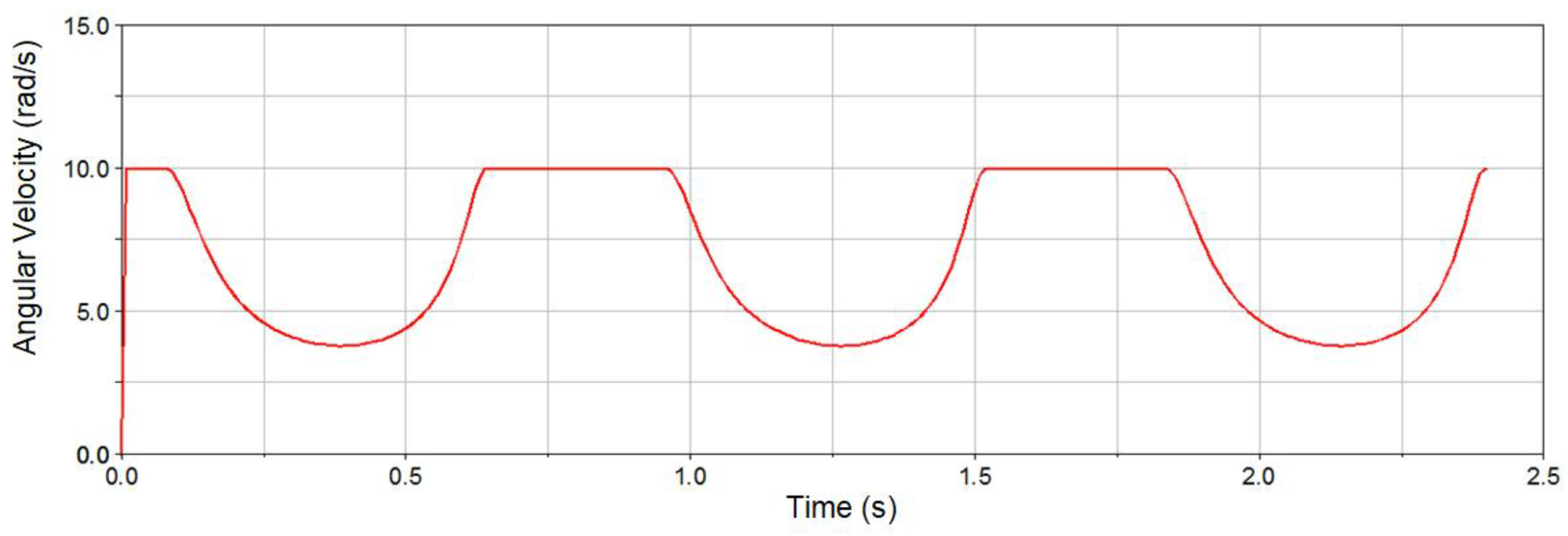
Figure 36.
Angular velocity variation of the drive joint during time.

Figure 37.
The node 610 elastic displacement vector component variation during time.

Figure 38.
Displacement and velocity variation for the marker no.: 13 depending on time.

Figure 39.
Variation diagrams for the engine torque and impact force components depending on time.

Publisher’s Note: MDPI stays neutral with regard to jurisdictional claims in published maps and institutional affiliations. |
© 2021 by the authors. Licensee MDPI, Basel, Switzerland. This article is an open access article distributed under the terms and conditions of the Creative Commons Attribution (CC BY) license (https://creativecommons.org/licenses/by/4.0/).
Share and Cite
MDPI and ACS Style
Dumitru, S.; Constantin, A.; Copilusi, C.; Dumitru, N. Impact Dynamics Analysis of Mobile Mechanical Systems. Mathematics 2021, 9, 1776. https://0-doi-org.brum.beds.ac.uk/10.3390/math9151776
AMA Style
Dumitru S, Constantin A, Copilusi C, Dumitru N. Impact Dynamics Analysis of Mobile Mechanical Systems. Mathematics. 2021; 9(15):1776. https://0-doi-org.brum.beds.ac.uk/10.3390/math9151776
Chicago/Turabian StyleDumitru, Sorin, Andra Constantin, Cristian Copilusi, and Nicolae Dumitru. 2021. "Impact Dynamics Analysis of Mobile Mechanical Systems" Mathematics 9, no. 15: 1776. https://0-doi-org.brum.beds.ac.uk/10.3390/math9151776
Note that from the first issue of 2016, this journal uses article numbers instead of page numbers. See further details here.