Approximation Solution for the Zener Impact Theory

Abstract

Collisions can be classified as completely elastic or inelastic. Collision mechanics theory has gradually developed from elastic to inelastic collision theories. Based on the Hertz elastic collision contact theory and Zener inelastic collision theory model, we derive and explain the Hertz and Zener collision theory model equations in detail in this study and establish the Zener inelastic collision theory, which is a simple and fast calculation of the approximate solution to the nonlinear differential equations of motion. We propose an approximate formula to obtain the Zener nonlinear differential equation of motion in a simple manner. The approximate solution determines the relevant values of the collision force, material displacement, velocity, and contact time.

1. Introduction

Theoretical research on collisions possesses significant value in engineering application. It is widely used in various industrial engineering fields—including aerospace, machinery, transportation, civil engineering, agriculture, and military applications. Collision is a mechanical phenomenon in which two or more objects in relative motion come into contact with each other for an instant, with changes in speed. Collisions are considered either elastic or inelastic based on the material properties and deformation types of the colliding objects. An elastic collision means that only elastic deformations occur in the colliding objects during collision, regardless of local contact deformation or if the entire deformed structure can be restored. Inelastic collisions mainly occur during crashing of metal objects in flexible systems. During these collisions, the structures of the colliding objects undergo elastic and plastic deformations at the local contact surfaces or overall systems. Therefore, even if the collision speed is low, the local contact stress exceeds the yield limit, thereby causing irreversible plastic deformation.

1.1. Hertz and Zener Impact Theory Related Studies

Hertz proposed a static contact problem for elastic bodies [1], where the spherical contact surface is approximated as a parabola. The two elastic balls contact problem was solved analytically. The colliding objects underwent elastic deformations during the elastic phase, which forms the basis of the Hertz elastic contact theory. The relationships between the contact force, deformation, and compression of the object were established to obtain the elastic collision contact time. Zener [2] extended the Hertz contact theory [1] and the effects of thin plate bending. To describe this model, let us consider the situation of a stationary plate or board impacted by a moving ball. In the Zener model, energy dissipation is considered only by bending waves propagating radially from the contact area [3]. The Zener model is not based on waves propagating through the thickness of the plate [4]; instead, it assumes that—during the collision of a large plate—the bending wave will not return to the contact area after being reflected from the lateral boundary of the plate. Additionally, it assumes that the radius of curvature of the large flat plate is greater and the contact radius is smaller than the thickness of the plate; that is, the sphere collides with the thin plate. While the sphere is in contact with the surface, quasi-longitudinal waves may propagate through the thickness of the board several times [2,5]. To calculate the rebound velocity of the ball, Zener [2] combined the equations of motion of the ball and the board—as described by Newton’s second law—to obtain the relationship between impulse and board displacements. Many scholars have subsequently continued their research based on the theoretical models of Hertz [1] and Zener [2,6]. Hunter [7] applied the kinetic energy transferred from the elastic longitudinal waves, etc., to the Hertz model [5] to consider the impact of small objects on infinite objects. Therefore, Hunter’s work was based on Hertz’s perfect elastic impact theory, ignoring all the attenuation effects caused by damping [7,8]. Boettcher et al. [8] modified the Hunter model [7] by considering the loss of kinetic energy during impact (Hunter loss) [7,8], they further modified the collision model proposed by Reed [9] to obtain more accurate elastic collision force–time parameters [5,8]. Mueller et al. [4] measured the coefficient of restitution and contact time for comparison with the theoretical predictions of the Hertz and Zener models. The contact time of the Hertz model does not consider the plate thickness as a parameter of influence. Hence, the model predicts the same result for a glass plate of any thickness [4], which is why the model is insufficient for predicting the contact time. The Hertz model can only accurately predict the contact time when the impact of a large plate is being considered [4,10]. Thus, the Hertz model represents a limiting case of the Zener model. In contrast, the contact time predicted by the Zener theoretical model approaches the actual measured value. The aforementioned research on collision is mostly based on the theories of the Hertz and Zener models.

1.2. Main Work and Purpose

In this study, we combined the Hertz contact theory and Zener inelastic collision models to propose a fast and straightforward method of deriving and establishing the Zener inelastic collision model. It is unnecessary to derive Newton’s second law from the beginning to obtain the Zener collision equation and hence the collision displacement, contact force, contact time, and speed. Another focus of this article is to provide a detailed review of the equations of the Hertz and Zener’s contact theory models for better understanding, along with their possible future applications for theoretical reference.

2. Review of Impact Mechanics

2.1. Hertz Model

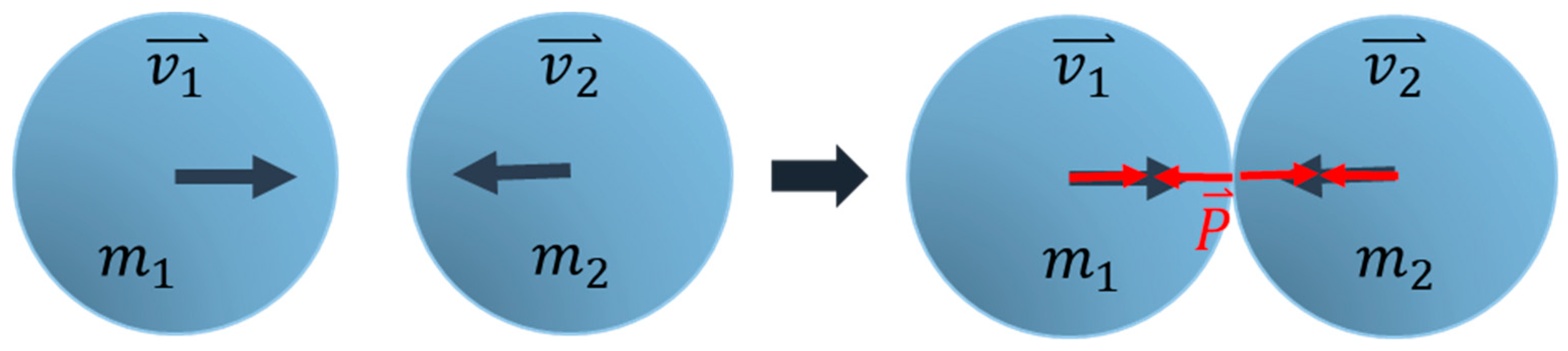
This section refers to Hertz (1882) [1] and Timoshenko and Goodier (1970) [11]. Hertz’s elastic collision theory [1] assumes that two spheres move linearly along their centers to cause a collision. The distance between the centers of the two spheres reduces gradually, and the speed of movement reduces to a static state. The collision that occurs at this moment causes the two spheres to produce the maximum amount of compression deformations. Finally, the two spheres gradually separate and return to their original conditions. This process is known as an elastic collision.

We assume that the masses of the two spheres are $m_1$ and $m_2$. The contact compression force $P$ is generated during collision, and the speed reduces and changes after collision. The velocities of the two spheres during collision are $\stackrel{\rightharpoonup }{v_1}$ and $\stackrel{\rightharpoonup }{v_2}$, as shown in Figure 1, and are expressed by Equation (1) according to Newton’s second law of motion.

$$m_1\frac{d\stackrel{\rightharpoonup }{v_1}}{dt}=-P, m_2\frac{d\stackrel{\rightharpoonup }{v_2}}{dt}=-P.$$

(1)

Assuming that the two spheres collide with the compression displacement $\stackrel{\rightharpoonup }{\alpha }$, the relative velocity of the spheres, $\stackrel{\rightharpoonup }{v_r}$, can be expressed by Equation (2) below.

$$\stackrel{\rightharpoonup }{v_r}=\frac{d\stackrel{\rightharpoonup }{\alpha }}{dt}=\stackrel{\rightharpoonup }{v_1}-\stackrel{\rightharpoonup }{v_2}=v_1\widehat{ı}+v_2\widehat{ı}=\left(v_1+v_2\right)\widehat{ı}.$$

(2)

From Equations (1) and (2), the relationship after collision of the spheres is

$$\frac{d\stackrel{\rightharpoonup }{v_r}}{dt}=\frac{d^2\stackrel{\rightharpoonup }{\alpha }}{d{t}^2}=\frac{d\stackrel{\rightharpoonup }{v_1}}{dt}-\frac{d\stackrel{\rightharpoonup }{v_2}}{dt}=-P\left[\frac{m_1+m_2}{m_1·m_2}\right]=-\frac{P}{M},$$

(3)

where $M=\frac{1}{\left(\frac{1}{m_1}+\frac{1}{m_2}\right)}=\frac{m_1·m_2}{m_1+m_2}$ is the effective (average) mass after collision of the spheres.

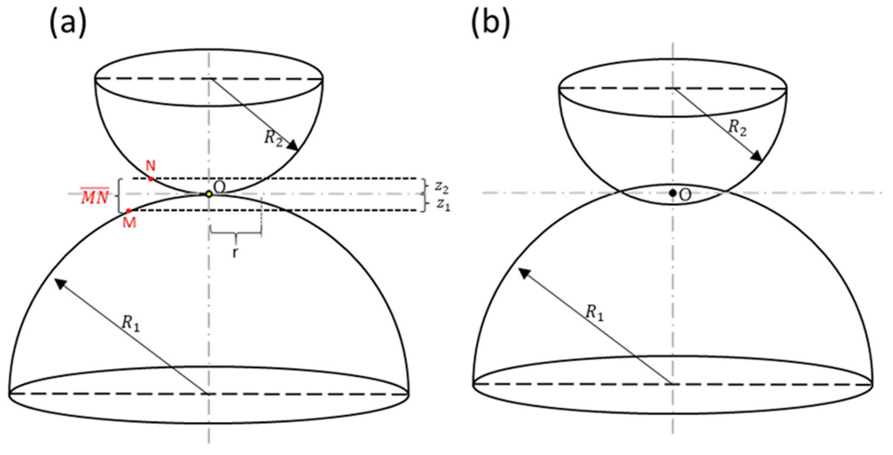
When the two spheres come into contact, as shown in Figure 2, the vertical distance between points $M$ and $O$ is $z_1$, and the vertical distance between points $N$ and $O$ is $z_2$; hence, $\overline{MN}$ distance can be expressed as Equation (4)

$$\overline{MN}=z_1+z_2=r^2\left(\frac{1}{2R_1}+\frac{1}{2R_2}\right)=\frac{r^2\left(R_1+R_2\right)}{2R_1{R}_2}.$$

(4)

When the two spheres collide, the elastic deformations $w_1$ and $w_2$ of the collision point change as shown in Figure 2a,b, and the contact surfaces of the two spheres are deformed. Therefore, the collision compression distance between the two spheres can be expressed by Equations (5) and (6) and are obtained using Equation (4).

$$\alpha =w_1+w_2+z_1+z_2,$$

(5)

$$w_1+w_2=\alpha -\beta r^2,$$

(6)

where $\alpha$ is the collision compression displacement between the centers of the two spheres after collision and $\beta =\frac{R_1+R_2}{2R_1{R}_2}$. Assuming that the maximum pressure intensity of a hemispherical collision is $q_0$ and that it is distributed on the surface of the hemisphere with radius $b$ at the point of contact, the total maximum collision compressive force $P$ can be expressed as in Equation (7).

$$P=\frac{q_0}{b}\frac{2}{3}\pi b^3=q_0\frac{2}{3}\pi b^2.$$

(7)

Here, $\alpha =\left(k_1+k_2\right)\frac{a{\pi }^2{q}_0}{2}$, $b=\left(k_1+k_2\right)\frac{{\pi }^2{q}_0}{4\beta }$, and $\beta =\frac{R_1+R_2}{2R_1{R}_2}$ can be obtained from Equations (7) and (6). Then, $\alpha$, $b$, and $\beta$ are applied in Equation (7) to obtain Equation (8).

$$\alpha ={\left[\frac{9{\pi }^2}{16}·\frac{P^2{\left(k_1+k_2\right)}^2\left(R_1+R_2\right)}{R_1{R}_2}\right]}^{\frac{1}{3}}.$$

(8)

Equation (9) can be obtained from Equation (8) as

$$P=n{\alpha }^{\frac{3}{2}},$$

(9)

where $\alpha$ is the contact displacement, $n$ is the Hertzian stiffness constant where $n=\frac{4}{3\pi \left(k_1+k_2\right)}\sqrt{\frac{R_1{R}_2}{R_1+R_2}}$.

Equation (9) is substituted with Equation (3) and updated as $d{\left(\frac{d\alpha }{dt}\right)}^2=2\frac{d^2\alpha }{d{t}^2}d\alpha$ to obtain Equation (10).

$$\frac{1}{2}\left[d{\left(\frac{d\alpha }{dt}\right)}^2\right]=-\frac{n}{M}{\alpha }^{\frac{3}{2}}d\alpha .$$

(10)

At the beginning of the collision, the compression is 0 and relative velocity is $v_0$. During the compression process, the relative speed is $v_r=\frac{d\alpha }{dt}$, and Equation (11) can be obtained by integrating Equation (10). At the end of the collision compression, the final relative speed is $v_r$ and maximum compression is ${\alpha }_{max}$.

$$\frac{1}{2}\left[{\left(\frac{d\alpha }{dt}\right)}^2-v_0{}^2\right]=-\frac{2}{5}\frac{n}{M}{\alpha }^{\frac{5}{2}} \Rightarrow v_0{}^2=\frac{4}{5}\frac{n}{M}{\alpha }_{max}{}^{\frac{5}{2}}\Rightarrow {\alpha }_{max}={\left[\frac{5}{4}\frac{M}{n}{v}_0{}^2\right]}^{\frac{2}{5}}.$$

(11)

Equation (11) gives time $t$ for the distance compression of the centroids of the two spheres and the maximum compression time $t_f$ of the two colliding bodies as

$$\frac{d\alpha }{dt}=\sqrt{v_0{}^2-\frac{4}{5}\frac{n}{M}{\alpha }^{\frac{5}{2}}}\Rightarrow dt=\frac{d\alpha }{v_0\sqrt{1-\frac{4}{5}\frac{n}{M{v}_0{}^2}{\alpha }^{\frac{5}{2}}}}$$

(12)

Suppose that at the initiation of the collision, the centers of the masses of the two spheres collide with a compression distance $\alpha =0$, $t=0$. For $x=0$ the maximum compression distance of the two collision bodies after collision is $={\alpha }_{max}$, $t=t_f$, where $x=1$, and $t_f$ is the end time of the collision. Let $x=\alpha /{\alpha }_{max}$, ${\alpha }_{max}dx=d\alpha$, after integrating Equation (12), the time $t$ required for compression of the distance between the centroids of the two spheres can be obtained through Equation (13).

$$dt=\frac{{\alpha }_{max}dx}{v_0\sqrt{1-\frac{4}{5}\frac{n}{M{v}_0{}^2}{\left({\alpha }_{max}x\right)}^{\frac{5}{2}}}}\Rightarrow t=\frac{{\alpha }_{max}}{v_0}{{\displaystyle \int }}_0^1\frac{dx}{\sqrt{1-x^{\frac{5}{2}}}}$$

(13)

Using the initial conditions of Equation (13), we obtain Equation (14).

$$\begin{gathered} \{\begin{array}{c}y=x^{\frac{5}{2}}\Rightarrow dx=\frac{2}{5}{y}^{-\frac{3}{5}}dy\\ x=0; y=0\\ x=1; y=1\end{array} \\ {t}_f=\frac{{\alpha }_{max}}{v_0}\frac{2}{5}{{\displaystyle \int }}_0^1{y}^{-\frac{3}{5}}{\left(1-y\right)}^{-\frac{1}{2}}dy. \end{gathered}$$

(14)

Using the beta function, ${\rm B}\left(m,n\right)={{\displaystyle \int }}_0^1{x}^{m-1}{\left(1-x\right)}^{n-1}dx=\frac{\mathsf{\Gamma }\left(m\right)\mathsf{\Gamma }\left(n\right)}{\mathsf{\Gamma }\left(m+n\right)}$, $m,n>0$ and gamma function, $\mathsf{\Gamma }\left(n\right){{\displaystyle \int }}_0^{\infty }{x}^{n-1}{e}^{1x}dx$, $\mathsf{\Gamma }\left(n-1\right)=n\mathsf{\Gamma }\left(n\right)=n!$, $n=1,2,3$. The maximum compression time of the colliding bodies of the two spheres ($t_f$) is given by Equation (15).

$$t_f =\frac{{\alpha }_{max}}{v_0}\frac{2}{5}\frac{\mathsf{\Gamma }\left(\frac{2}{5}\right)\mathsf{\Gamma }\left(\frac{1}{2}\right)}{\mathsf{\Gamma }\left(\frac{2}{5}+\frac{1}{2}\right)}=1.47\frac{{\alpha }_{max}}{v_0}.$$

(15)

The Hertz perfect elastic collision time is $2t_f$ and is given as in Equation (16)

$$2t_f=2.94\frac{{\alpha }_{max}}{v_0}=2.94{\left[\frac{5}{4}\frac{M}{n}{v}_0{}^2\right]}^{\frac{2}{5}}\frac{1}{v_0}=3.215{\left(\frac{M}{n{v}_0{}^{\frac{1}{2}}}\right)}^{\frac{2}{5}}=3.215{\left(T\right)}^{\frac{2}{5}},$$

(16)

where $T=\frac{M}{n{v}_0{}^{\frac{1}{2}}}$.

2.2. Zener Model

This section refers to Zener (1941) [2]. When a collision occurs between two spheres, it is generally not completely elastic, as assumed in Hertz theory [1]. Because of the energy consumed during a collision, inelastic collision occurs instead. During the impact, pressure is generated in the contact area. Local deformation causes a stress wave, which propagates inward through the object from the excitation point [4]. In addition, the generation of collision waves from the surfaces of the object and body can cause energy loss at the impact area. Elastic waves propagate through solids and exhibit characteristic velocities. Therefore, multiple refractions or reflections of waves at the interface cause energy dissipation. The Hertz model [1] is a conservative force field; hence, it does not consider the energy consumption during actual collision. As a result, there is a gap in the analysis results of actual collisions.

Zener [2] extended the Hertz theory through the bending effect of the board; thus, it is assumed that the board extends infinitely in the horizontal direction. The Zener model describes a sphere hitting a thin plate, and as per the model, bending waves do not return to the contact area after reflecting from the lateral boundary of the plate. Zener [2] combined the sphere and plate motion equations explained by Newton’s second law to describe the interaction between the bending effect of the ball colliding with the plate and its process.

First, we assume that the radius of curvature of the plate and the angle between the plate and arrival plate overall are small. However, it is large compared to its thickness. For the theory of thin plates with the reaction to localized impulsivity, the transverse displacement $U\left(x,y,t\right)$ of the plate can be represented by the differential equation

$$\left(D{\nabla }^4+2\rho h\frac{d^2}{d{t}^2}\right)U=f,$$

(17)

where $f$ is the surface density of the normal force, $\rho$ is the density, $2h$ is the thickness of the plate, $D=\frac{2}{3}{h}^3\frac{E}{1-{\nu }^2}$ the rigidity modulus, and ν is Poisson’s ratio of the impacting bodies.

$$\begin{gathered} {\nabla }^2:\frac{{\partial }^2}{\partial x^2}+\frac{{\partial }^2}{\partial y^2}, {\nabla }^4:\frac{{\partial }^4}{\partial x^4}+2\frac{{\partial }^4}{\partial x^2\partial y^2}+\frac{{\partial }^4}{\partial y^4}. \\ \mathrm{Let} U\left(x,y,t\right)={{\displaystyle \sum }}_n{C}_n\left(t\right)U_n\left(x,y\right), \end{gathered}$$

(18)

where $C_n\left(t\right)$ is an eigenvalue, and $U_n\left(x,y\right)$ are normalized eigenfunctions. Substituting Equation (18) into Equation (17) and multiplying by $U_k$, with $dA$ being integrated over the surface of plate, we get Equation (19).

$$2\rho h{\omega }_k{}^2{C}_k={\displaystyle \int }{U}_{k}fdA=U_k\left(0\right)F\left(t\right),$$

(19)

where ${\omega }_k$ and $U_k$ are the eigenvalues and normalized eigenfunctions, respectively. $U_k\left(0\right)$ is the value of $U_k$ at the point of application of force $F\left(t\right)$, which gives $C_k={\left(2\rho h{\omega }_k\right)}^{-1}{U}_k\left(0\right){{\displaystyle \int }}_0^{t}F\left(t^{\prime }\right)\sin {\omega }_k\left(t-t^{\prime }\right)d{t}^{\prime }$. For the integral of $t^{\prime }$, as long as $t$ is sufficiently small, the boundaries do not reflect the disturbance. Hence, this integration process does not depend on the shape of the plate and boundary conditions.

$$U\left(0,t\right)={{\displaystyle \sum }}_n{C}_n\left(t\right)U_n\left(0\right),$$

(20)

$$={\left(2\rho h\right)}^{-1}{{\displaystyle \sum }}_n{\omega }_n{}^{-1}{U}_n{}^2\left(0\right){{\displaystyle \int }}_0^{t}F\left(t^{\prime }\right)\sin {\omega }_n\left(t-t^{\prime }\right)d{t}^{\prime },$$

(21)

$$=\xi {{\displaystyle \int }}_0^{t}F\left(t^{\prime }\right)d{t}^{\prime },$$

(22)

where the $\xi$ is the bending coefficient given as

$$\xi =\frac{{\left(\frac{3\rho }{E^{\prime }}\right)}^{\frac{1}{2}}}{16\rho h^2},$$

(23)

Here, $h$ is the plate thickness, $\rho$ is the density of the plate, and $E^{\prime }$ is the modulus of elasticity of the plate.

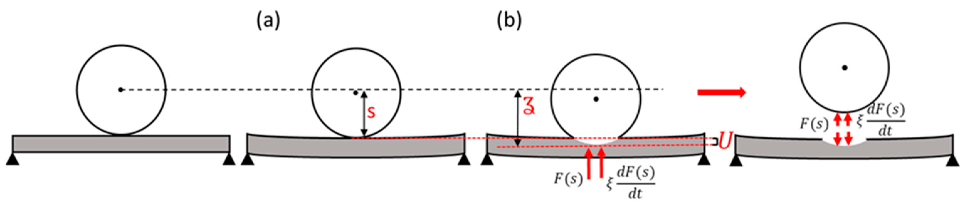
Suppose that when a sphere hits the plate, as it falls freely from a height, the ball and plate collide through an ideal elastic collision, and the total displacement $\left(s\right)$ is as shown in Figure 3a. On the other hand, in the case of an inelastic collision, the total displacement caused by the actual collision is $(ʓ)$, and the irreversible deformation of the plate after collision is $\left(U\right)$, as shown in Figure 3b. The total displacements of the elastic and inelastic collisions are as follows.

$$ʓ=s+U.$$

(24)

The acceleration obtained using the second differential of the displacement in Equation (24) as well as Equations (1) and (23) gives Zener’s nonlinear motion equation as

$$\frac{d{s}^2}{d{t}^2}+\frac{1}{M}F\left(s\right)+\xi \frac{dF\left(s\right)}{dt}=0.$$

(25)

The nonlinear differential equation proposed by Zener [2] is transformed to provide an analytical solution by simplifying the Hertzian contact force as a function of the displacement. Thus, Equation (9) is rewritten as

$$\frac{d{s}^2}{d{t}^2}+\frac{1}{M}F\left(s\right)+\xi \frac{dF\left(s\right)}{dt}=0.$$

(26)

where $s$ is the contact displacement, $k$ is the Hertzian stiffness constant, and Equation (26) can be written in dimensionless form using transformations $\sigma \left(\tau \right)=\frac{s\left(t\right)}{T{v}_0}$ and $\tau =\frac{t}{T}$; $\sigma$ and $\tau$ are dimensionless displacement and time, respectively; $t$ is the time and $T$ is a characteristic time constant that reflects the mechanical material properties of the sphere and plate as

$$T={\left(\frac{M}{n{v}_0{}^{\frac{1}{2}}}\right)}^{\frac{2}{5}}.$$

(27)

Equation (25) can be transformed into a dimensionless differential equation of Equation (28), which is given as [2]

$$\frac{d^2\sigma }{d{\tau }^2}+\left(1+\lambda \frac{d}{d\tau }\right){\sigma }^{\frac{3}{2}}=0.$$

(28)

According to Zener [2], all parameters that influence the impact are summarized using a dimensionless inelasticity parameter, $\lambda$, as per Equation (29)

$$\lambda =\xi k{v}_0{}^{\frac{1}{2}}{T}^{\frac{3}{2}}=\xi M\left(\frac{k}{M}{v}_0{}^{\frac{1}{2}}{T}^{\frac{3}{2}}\right)=\xi M\left(T^{-\frac{5}{2}}·T^{\frac{3}{2}}\right)=\frac{\xi M}{T}.$$

(29)

3. Results and Discussion

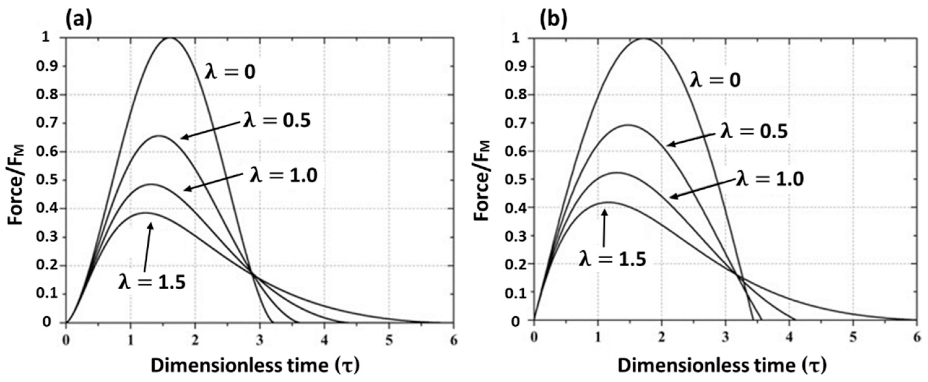
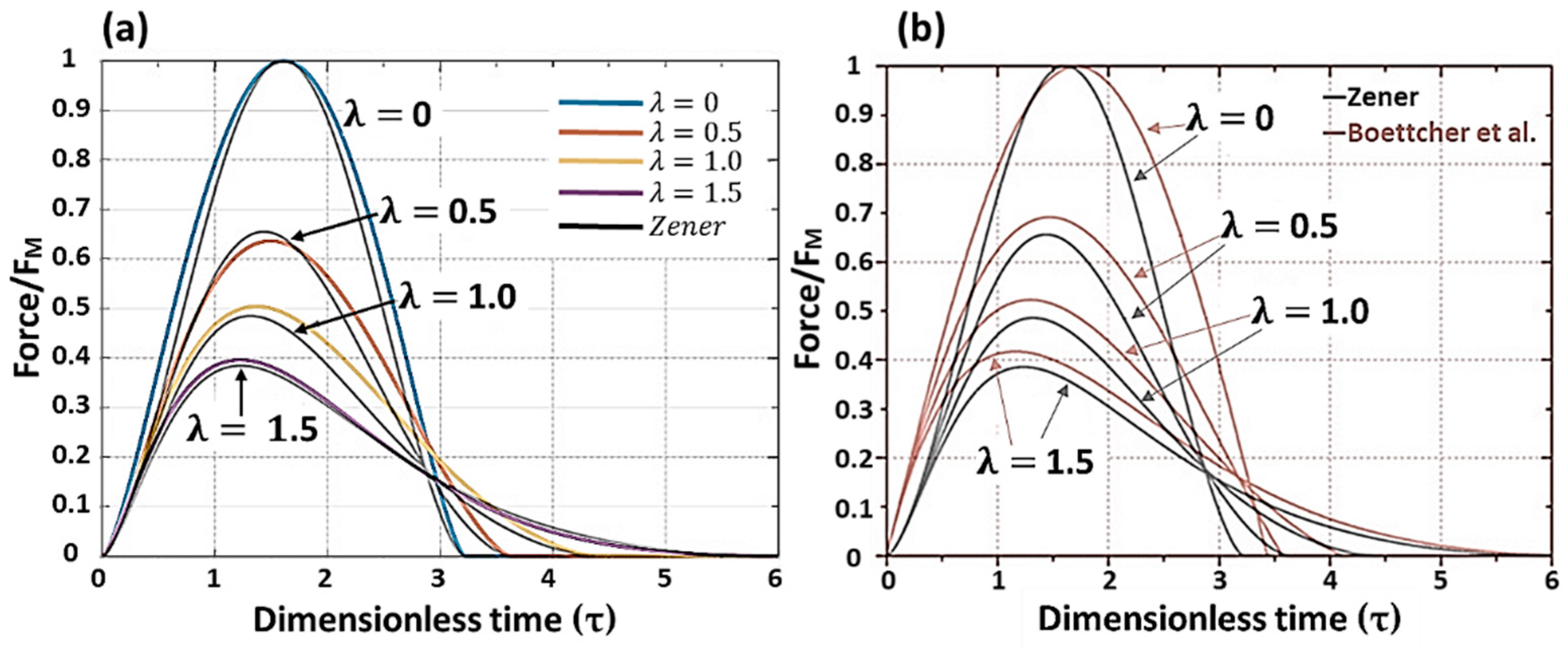
When the ball collides with the plate material, the inelasticity parameter ($\lambda$) between the two and force time during the impact change owing to different material properties. The Zener collision theory equation was numerically analyzed and complex calculations were performed. Furthermore, the force–time collision curve diagram was drawn with $\lambda$ at 0, 0.5, 1.0, and 1.5, as shown in Figure 4a. Figure 4a shows the process of change in the impact contact time and the magnitude of the contact force. Through the Hertzian contact force as a function of the displacement (Equation (26)), the impact force was converted to material displacement and other parameters. Next, the material inelasticity parameter ($\lambda$) was calculated using Equation (29).

Boettcher et al. [12] revised the nonlinear motion equation (Equation (25)) [2] proposed by Zener with a dimensionless parameter, ${\omega }_0$, to be adjusted (determined by adapting the ${\omega }_0$ dimensionless analytical displacement–time function), and Hertz’s equation (Equation (26)) [1], and established a method that simply analyzes the nonlinear motion equation of the Zener collision [3,12]. Boettcher et al. also simplified the Zener nonlinear collision equation (Equation (28)) to a linear differential equation, which can be regarded as a damped oscillation equation. When $\lambda =0$, an ideal elastic collision without damping is indicated, whereas $\lambda >0$ is an inelastic collision and has a damping state [12]. The process obtains the force–time impact curve of $\lambda =0$, which is a perfect elastic collision equation, and then adjusts ${\omega }_0$ to obtain $\lambda >0$, that is, the inelastic collision [3,12]. Figure 4b shows the normalized impact force curve obtained by Boettcher et al. after a simplified analysis of Zener’s nonlinear motion equation [12]. This work is based on the nonlinear motion equation provided by Zener [2], which establishes the force–time collision curve equation in different ways.

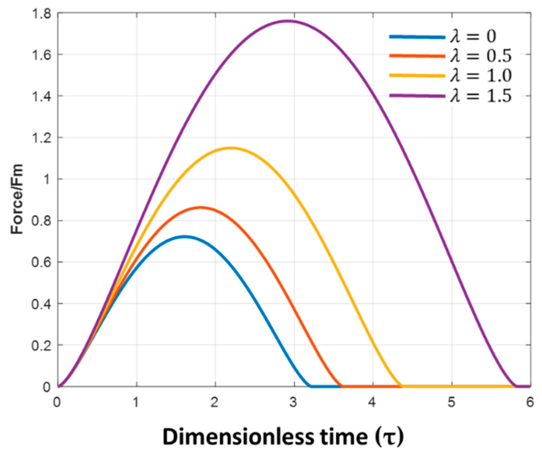
As observed in Figure 4, the sphere collides with the plate, and the contact force changes with time. Additionally, the force ascends from zero to the maximum value and then decreases gradually. It is considered to be an ideal elastic collision when the inelasticity parameter is zero. The impact process is not affected by the friction force and causes energy attenuation. Consequently, the force–time variation curve is a symmetrical graph. When the inelasticity parameter is larger ($\lambda \ne 0$), it is an inelastic collision. Energy loss was generated during the collision between the sphere and the plate, and the contact force was smaller, while the contact time was longer. As seen in Figure 4, the force–time collision curve based on Equation (28) correlates well with the dimensionless displacement ($\sigma$) and time ($\tau$). As shown in Figure 5, the force–time curve is a graph of the quadratic function. First, we used the approximation method, and the curve was drawn based on Equation (30).

$$\frac{Force}{F_m}={\sigma }^{\frac{3}{2}}={\left[\tau \left(1-\frac{\tau }{{\tau }_{el}}\right)\right]}^{\frac{3}{2}}.$$

(30)

The relationship between the elastic collision time (τ) and the inelasticity parameter ($\lambda$) of the plate is based on the equation ${\tau }_{el}=2.762+0.4568e^{1.27\lambda }$ provided by Müller et al. [4]. Additionally, the displacement ($\sigma$) can be converted into force using Equation (26). Equation (30) provides the left–right symmetrical quadratic function graph. When the elasticity parameter is 0, it is an elastic collision curve. Consequently, the inelasticity parameter value ($\lambda \ne 0$) and impact force are greater and the contact time is longer, as shown in Figure 5.

However, in the actual collision process, $\lambda \ne 0$. After the sphere collides with the plate, the force on the plate shows an exponential attenuation as the sphere leaves the plate. Therefore, we multiply the $\sigma$ in Equation (30) by $e^{-\lambda \tau }$ to obtain Equation (31), as

$$\frac{Force}{F_m}={\sigma }^{\frac{3}{2}}={\left[\tau \left(1-\frac{\tau }{{\tau }_{el}}\right)e^{-\lambda \tau }\right]}^{\frac{3}{2}}.$$

(31)

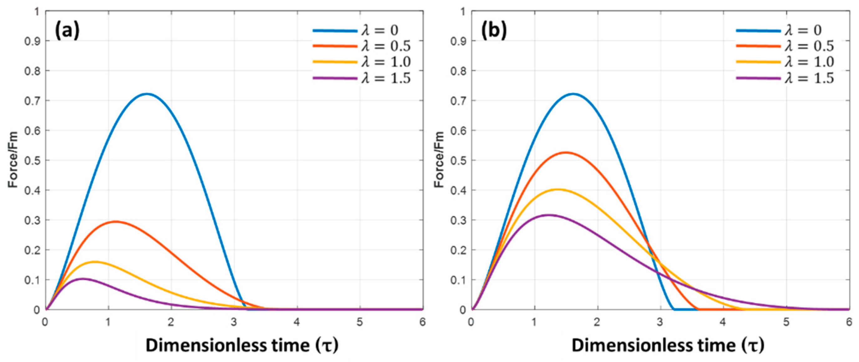
Equation (31), as seen from Figure 6a, shows an exponential decay change with time in the force process of different inelasticity parameter materials. The selection range of $e^{-\lambda \tau }$ coefficient is from $e^{-0.3\lambda \tau }$ to $e^{-0.5\lambda \tau }$. When multiplied by $e^{-0.4\lambda \tau }$, the force is an attenuated process of the contact time. As per the comparison curve between Figure 6b and the $\sigma$ of Equation (30) multiplied by $e^{-0.4\lambda \tau }$ and Figure 4a, Zener’s standard force–time collision curve is the closest.

Figure 6b shows that $\lambda =0$, and the maximum collision force ($\mathit{Force}/F_m$) is not equal to 1. Therefore, the correction Equation (31), multiplied by $\frac{4}{{\tau }_{el}}$, aims to correct the change in contact time and force of different inelasticity parameters, and the force ($\mathit{Force}/F_m$) of $\lambda =0$ can be corrected to 1, as shown in Figure 7a.

$$\frac{Force}{F_m}={\sigma }^{\frac{3}{2}}={\left[\frac{4\tau }{{\tau }_{el}}\left(1-\frac{\tau }{{\tau }_{el}}\right)e^{-0.4\lambda \tau }\right]}^{\frac{3}{2}}.$$

(32)

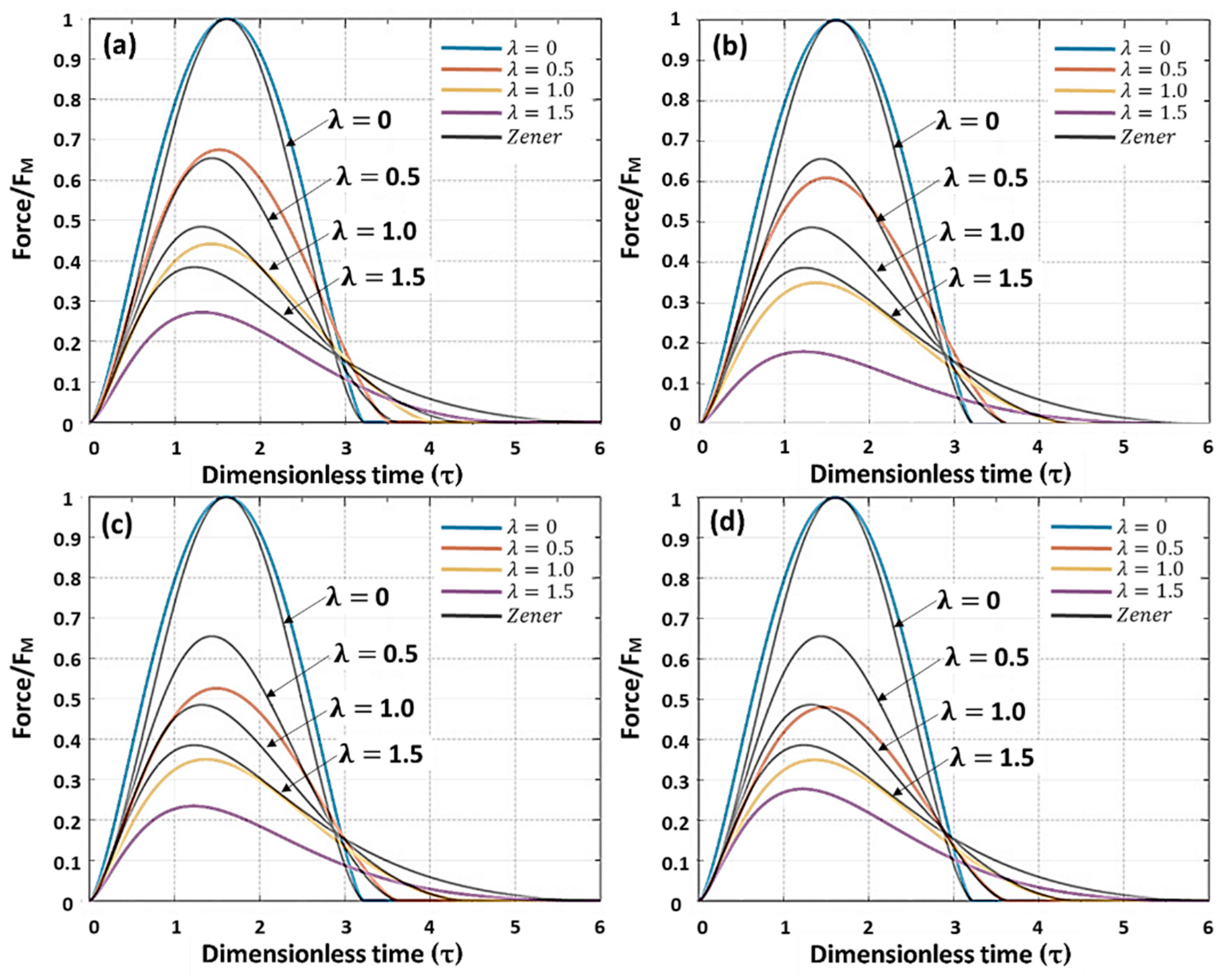
The force–time collision curve of Equation (32) is quite close to the original Zener force–time diagram (Figure 4), as shown in Figure 7a. However, when the inelasticity parameters are 1 and 1.5, the maximum force curve is very different from the Zener curve; hence, we multiply the $\sigma$ in Equation (32) by $({\lambda }^n+\left(1-\lambda \right))$ to modify the same, as shown in Equation (33).

$$\frac{Force}{F_m}={\sigma }^{\frac{3}{2}}={\left[({\lambda }^n+\left(1-\lambda \right))\frac{4\tau }{{\tau }_{el}}\left(1-\frac{\tau }{{\tau }_{el}}\right)e^{-0.4\lambda \tau }\right]}^{\frac{3}{2}}.$$

(33)

When the $\sigma$ of Equation (32) is multiplied by $({\lambda }^n+\left(1-\lambda \right))$, the force–time curve with n > 0 and $\lambda =1$ does not change, as shown in Figure 7b–d. However, when the value of n in Equation (33) becomes larger, and $\lambda =0.5$, the impact force curve gradually becomes smaller, whereas for $\lambda =1.5$, it gradually becomes larger, as shown in Figure 7b–d. Additionally, the value of n gradually increases from 1.0, 1.3, and 1.5 for comparison. Finally, the value of $\mathrm{n}=1.3$ is the maximum force peak value of the force–time curve drawn using Equation (33) established in this study is between the peak force value of the inelasticity parameter 0.5 to 1.5 and the Zener value, and the peaks of the force–time curve are equidistant, as shown in Figure 7c.

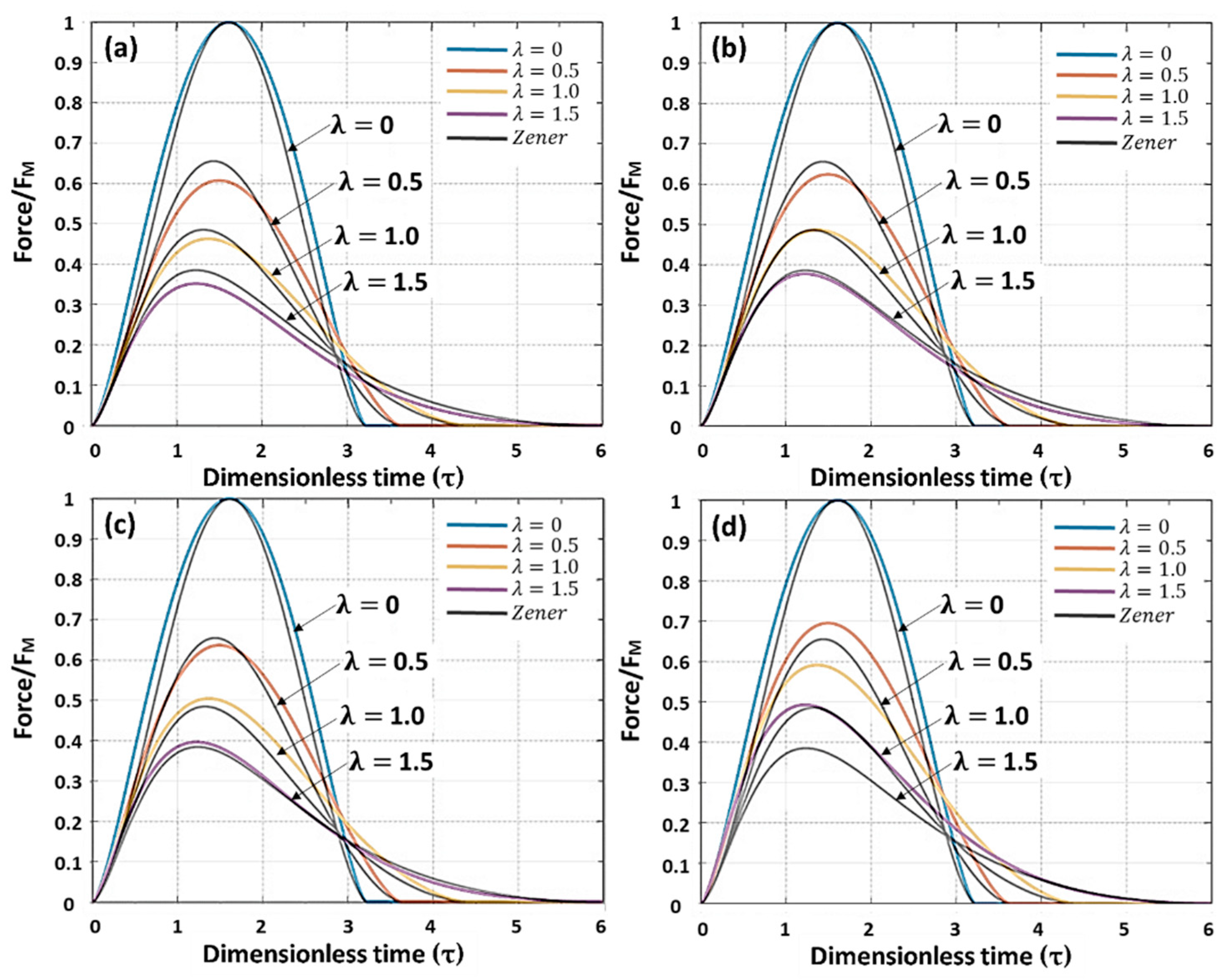
As shown in Figure 7c, the force–time curve peak values of the inelasticity parameters 0.5–1.5 are approximately equidistant from the Zener force–time curve peak values. Therefore, the correction Equation (33) adjusts the peak force of the force–time curve and multiplies it by ${\left(1+\mathrm{n}\times \lambda \right)}^2$ to provide Equation (34).

$$\frac{Force}{F_m}={\sigma }^{\frac{3}{2}}={\left(1+\mathrm{n}\times \lambda \right)}^2{\left[({\lambda }^{1.3}+\left(1-\lambda \right))\frac{4\tau }{{\tau }_{el}}\left(1-\frac{\tau }{{\tau }_{el}}\right)e^{-0.4\lambda \tau }\right]}^{\frac{3}{2}}.$$

(34)

When $\lambda =0$, ${\left(1+\mathrm{n}\times \lambda \right)}^2$, n is any value, the force is 1, and the force–time curve remains constant. Thus, the inelasticity parameter is between 0.5 and 1.5. When the value of n in Equation (34) is larger, the force–time curve of the inelasticity parameter gradually increases the force value, as shown in Figure 8. When $\mathrm{n}=0.2$, it is nearly identical to the time–force curve of the original Zener, and the curve drawn with inelasticity parameters of 1–1.5 uses Equation (34). Therefore, $\mathrm{n}=0.2$ is the most suitable. As shown in Figure 9a,b, the force–time collision curve given using Equation (34) and that given by Boettcher et al. are different from the analytical methods that provide graphs and equations that are considerably similar to the diagrams of the force–time collisions proposed by Zener.

4. Conclusions

The nonlinear collision motion equation proposed by Zener [2] is the force–time collision curve of the inelasticity parameter ($0\le \lambda \le 1.5$) considered in the collision process through numerical analysis. In this study, we have proposed an approximate solution to Zener’s inelastic collision theory, which is expressed as

$$\frac{Force}{F_m}={\sigma }^{\frac{3}{2}}={\left(1+0.2\lambda \right)}^2{\left[({\lambda }^{1.3}+\left(1-\lambda \right))\frac{4\tau }{{\tau }_{el}}\left(1-\frac{\tau }{{\tau }_{el}}\right)e^{-0.4\lambda \tau }\right]}^{\frac{3}{2}}.$$

The contribution of the present study to literature includes an approximate solution that is simple and can be used directly without complex calculations. The contact time, magnitude of the material impact force and displacement, and inelasticity parameter can be obtained simply by substituting the parameters into the equation. Using the approximate solution, the inelasticity parameter can be obtained from the thickness, density, and modulus of elasticity of the material, and the relationship between thickness and contact time can be obtained by simple and fast calculation. Furthermore, the method can be applied to nondestructive impact quality inspections of commercial materials, such as internal defects and thickness differences of liquid crystal glass panels. It can also be applied to the quality inspection of golf club heads in the future. In summary, the use of the proposed formula does not require complex numerical calculations and can be verified easily to obtain the collision-related parameters. Furthermore, the proposed approximate solution can be adjusted for application based on user requirements.

References

- Hertz, H. Ueber die Berührung fester elastischer Körper. J. Für Die Reine Und Angew. Math. 1882, 1882, 156–171. [Google Scholar] [CrossRef]
- Zener, C. The Intrinsic Inelasticity of Large Plates. Phys. Rev. 1941, 59, 669–673. [Google Scholar] [CrossRef]
- Boettcher, R.; Russell, A.; Mueller, P. Energy dissipation during impacts of spheres on plates: Investigation of developing elastic flexural waves. Int. J. Solids Struct. 2017, 106–107, 229–239. [Google Scholar] [CrossRef]
- Müller, P.; Böttcher, R.; Russell, A.; Trüe, M.; Aman, S.; Tomas, J. Contact time at impact of spheres on large thin plates. Adv. Powder Technol. 2016, 27, 1233–1243. [Google Scholar] [CrossRef]
- Jebelisinaki, F.; Boettcher, R.; van Wachem, B.; Mueller, P. Impact of dominant elastic to elastic-plastic millimeter-sized metal spheres with glass plates. Powder Technol. 2019, 356, 208–221. [Google Scholar] [CrossRef]
- Koller, M.G.; Kolsky, H. Waves produced by the elastic impact of spheres on thick plates. Int. J. Solids Struct. 1987, 23, 1387–1400. [Google Scholar] [CrossRef]
- Hunter, S.C. Energy absorbed by elastic waves during impact. J. Mech. Phys. Solids 1957, 5, 162–171. [Google Scholar] [CrossRef]
- Boettcher, R.; Kunik, M.; Eichmann, S.; Russell, A.; Mueller, P. Revisiting energy dissipation due to elastic waves at impact of spheres on large thick plates. Int. J. Impact Eng. 2017, 104, 45–54. [Google Scholar] [CrossRef]
- Reed, J. Energy losses due to elastic wave propagation during an elastic impact. J. Phys. D Appl. Phys. 1985, 18, 2329–2337. [Google Scholar] [CrossRef]
- Stevens, A.B.; Hrenya, C.M. Comparison of soft-sphere models to measurements of collision properties during normal impacts. Powder Technol. 2005, 154, 99–109. [Google Scholar] [CrossRef]
- Timoshenko, S.P.; Goodier, J.N. Theory of Elasticity, 3rd ed.; McGraw-Hill: New York, NY, USA, 1970. [Google Scholar]
- Böttcher, R.; Müller, P.; Trüe, M.; Russell, A.; Tomas, J. Energiedissipation aufgrund von Biegewellen bei Stoßvorgängen gegen dünne Platten. Chem. Ing. Tech. 2016, 88, 1002–1011. [Google Scholar] [CrossRef]
Figure 1.
Schematic illustration of the elastic collision of two spheres.
Figure 2.
Schematic of compression changes after collision of two balls (a) coming into contact with each other and (b) colliding with each other.
Figure 3.
Ball collides with a plate via (a) elastic and (b) inelastic collisions.
Figure 4.
(a) Zener standard force–time collision curve [2,12]. (b) Boettcher et al. simplified the normalized force–time collision curve graph obtained from the analysis of the Zener equation [12].
Figure 5.
Force–time change quadratic function curve.
Figure 6.
The of Equation (30) is multiplied by (a) and (b) .
Figure 7.
(a) The of Equation (31) is multiplied by . Multiplying the σ in Equation (32) by (b) , (c) , (d) .
Figure 8.
Equation (33) multiplied by , when (a) n = 0.15, (b) n = 0.18, (c) n = 0.2, and (d) n = 0.3.
Publisher’s Note: MDPI stays neutral with regard to jurisdictional claims in published maps and institutional affiliations. |
© 2021 by the authors. Licensee MDPI, Basel, Switzerland. This article is an open access article distributed under the terms and conditions of the Creative Commons Attribution (CC BY) license (https://creativecommons.org/licenses/by/4.0/).
Share and Cite
MDPI and ACS Style
Tsai, P.-K.; Li, C.-H.; Lai, C.-C.; Huang, K.-J.; Cheng, C.-W. Approximation Solution for the Zener Impact Theory. Mathematics 2021, 9, 2222. https://0-doi-org.brum.beds.ac.uk/10.3390/math9182222
AMA Style
Tsai P-K, Li C-H, Lai C-C, Huang K-J, Cheng C-W. Approximation Solution for the Zener Impact Theory. Mathematics. 2021; 9(18):2222. https://0-doi-org.brum.beds.ac.uk/10.3390/math9182222
Chicago/Turabian StyleTsai, Ping-Kun, Cheng-Han Li, Chia-Chun Lai, Ko-Jung Huang, and Ching-Wei Cheng. 2021. "Approximation Solution for the Zener Impact Theory" Mathematics 9, no. 18: 2222. https://0-doi-org.brum.beds.ac.uk/10.3390/math9182222
Note that from the first issue of 2016, this journal uses article numbers instead of page numbers. See further details here.