Reliability and Inference for Multi State Systems: The Generalized Kumaraswamy Case

Abstract

Semi-Markov processes are typical tools for modeling multi state systems by allowing several distributions for sojourn times. In this work, we focus on a general class of distributions based on an arbitrary parent continuous distribution function G with Kumaraswamy as the baseline distribution and discuss some of its properties, including the advantageous property of being closed under minima. In addition, an estimate is provided for the so-called stress–strength reliability parameter, which measures the performance of a system in mechanical engineering. In this work, the sojourn times of the multi-state system are considered to follow a distribution with two shape parameters, which belongs to the proposed general class of distributions. Furthermore and for a multi-state system, we provide parameter estimates for the above general class, which are assumed to vary over the states of the system. The theoretical part of the work also includes the asymptotic theory for the proposed estimators with and without censoring as well as expressions for classical reliability characteristics. The performance and effectiveness of the proposed methodology is investigated via simulations, which show remarkable results with the help of statistical (for the parameter estimates) and graphical tools (for the reliability parameter estimate).

1. Introduction

The Kumaraswamy distribution is a well-known distribution, especially to those familiar with the hydrological literature [1]. Kumaraswamy’s densities are unimodal and uniantimodal and, depending on the parameter values chosen, are either increasing or decreasing or constant functions. Note that most if not all of the above characteristics are shared by both Kumarasawmy and Beta distributions (see [2,3,4]). In fact, Kumarasawmy and Beta distributions share numerous characteristics, although some of them are much more readily available, from the mathematical point of view, for the Kumaraswamy distribution. Kumaraswamy distribution is appropriate for the modeling of bounded natural and physical phenomena, such as atmospheric temperatures or hydrological measurements [5,6], record data, such as tests, games or sports [7], economic observations [8], or for empirical data with failure rate with an increasing prior [9]. It is also appropriate in situations where one considers a distribution with infinite lower and/or upper bounds to fit data, when, in fact, the bounds are finite, which makes Kumaraswamy useful in preventive maintenance. Some specific examples discussed in the literature include failure and running times of devices [10] and deterioration or fatigue failure [11]. Furthermore, due to the closed form of both its distribution as well as its quantile function (inverse cumulative distribution), Kumaraswamy appears advantageous when it comes to the quantile modeling perspective [12,13]. These characteristics make Kumaraswamy useful and easily applicable in reliability theory.

A general class of distributions with Kumaraswamy as a baseline distribution is considered in this work by using a parent continuous distribution function: $G(·)$. The Kumaraswamy distribution is viewed as the baseline distribution of the proposed G-class because it arises in the trivial case associated with $G\left(x\right)$ being the identity function, which corresponds to the $U(0,1)$ parent distribution. For an arbitrary continuous parent distribution, one can generate a general subclass of distributions with the support that is different from the support of the baseline distribution (i.e., the Kumaraswamy distribution), distribution that is defined like the Beta distribution, in $[0,1]$. The general form of the G-class of distributions based on an arbitrary parent cdf $G(·),$ with Kumaraswamy as the baseline distribution, is defined by the following (see [2,14,15,16]):

$$\begin{array}{c}\hfill F(t;a)=1-{(1-{G\left(t\right)}^c)}^a,c,a>0,\end{array}$$

(1)

where both parameters c and a are considered shape parameters associated with the skewness and a tail weight of $F(·)$. Note that additional structural parameters associated with $F(·)$ (such as the shape parameter c) and/or distributional parameters associated with the parent distribution $G(·)$ may also be involved in (1). Due to the fact that the distribution function in (1) is written in a closed form, it can be effectively used for both uncensored and censored data in reliability theory as well as in survival analysis.

The statistical inference, including parameter estimation in the context of reliability modeling, is of vital importance. In addition to the use of a proper distribution, such as (1), for modeling purposes, one may also be interested in evaluating the performance of the reliability system involved. Indeed, for instance, the problem of performance of a system is of great importance in mechanical engineering and refers to a component of strength X, which is subject to stress Y. The system stays in operation as long as the stress is less than the strength, so the system performance is associated with the probability of exceedance, usually denoted by R. The quantity of interest in such cases is the stress–strength reliability or reliability parameter which is a measure of reliability defined by the following:

$$\begin{array}{c}\hfill R=\mathbb{P}(Y<X)=\mathbb{E}\left[\mathbb{P}\right(Y<X\left)\right|X].\end{array}$$

(2)

The concept of stress–strength reliability has been investigated extensively in the literature for various lifetime distributions. The reliability parameter has been obtained for several distributions that typically appear in reliability analyses, such as Exponential, Gamma, Weibull, Burr, Marshall–Olkin extended Lomax distribution and inverse Rayleigh distribution. Such distributions were considered for at least one of the two variables of interest, namely X and Y (see [17,18,19,20,21]).

In this work, we focus on the general class of distributions of the form (1), using a parent continuous distribution function, and discuss some of its properties, including the stress–strength reliability. In addition, and for a multi-state system, we provide parameter estimates for the class given in (1), which are assumed to vary over the states of the system. The theoretical part of the work also includes the asymptotics for the proposed estimators. The performance of the proposed methodology is investigated with simulated results.

The paper is organized as follows: In Section 2, we propose and discuss the G-class of distributions (1). In Section 3 and Section 4, the semi-Markov setting and the parameter estimation are provided. Reliability characteristics are discussed in Section 5, while applications are analyzed in the final section.

2. The G-Class of Distributions

Consider the family of distributions with shape parameter a and distribution function, given by the following:

$$\begin{array}{c}\hfill F(t;a):=1-{\left(1-F(t;1)\right)}^a,\end{array}$$

(3)

which is absolutely continuous w.r.t. the Lebesgue measure, with density function $f(t;a)$ and with $F(t;1)$ being the standard family member when $a=1$. Classical reliability distributions, such as Exponential, Rayleigh and Weibull distributions are members of (3). One of the special features of (3) is that the distribution of the minimum, i.e., of the ordered statistic $X_{\left(1\right)}$ of a random sample $X_1,X_2,\dots ,X_n$ from (3), falls within this class (see [22,23]).

Notice that the general G-class of distributions in (1) with a parent continuous distribution $G(·)$ builds a new general class of distributions with each member lying within the class given in (3), with

$$F(t;1)=G^c\left(t\right)$$

and Kumaraswamy as the baseline distribution of the entire class. It should be noted that the baseline (Kumaraswamy) distribution is obtained for the Uniform distribution in $[0,1]$, i.e., for the identity function $G\left(x\right)=x$, with cdf provided by the following expression:

$$\begin{array}{c}\hfill F_K(t;a):=1-{\left(1-t^c\right)}^a,t\in (0,1).\end{array}$$

(4)

Note that the Kumaraswamy distribution is a member of the G-class (1) with $F_K(t;1)=t^c$. Kumaraswamy distribution, which, due to the form of the function G, can be viewed as a Generalized Uniform distribution, is an easy to handle distribution in the sense that it has simple explicit expressions for the distribution and quantile functions as well as the L-moments and the moments of order statistics [2]. Furthermore, it has a simple formula for the generation of random samples. The proposed general G-class though, goes beyond the Kumaraswamy since for each (any) continuous distribution chosen as the parent distribution G (i.e., Exponential, Gamma, Weibull, Gumbel, Rayleigh, and Inverse Gaussian), a new special/specific general (sub)class of densities arises (Generalized Exponential, Gamma, Weibull, Gumbel, Rayleigh or Inverse Gaussian, etc.). Observe that each of these general specific subclasses offers additional flexibility to the researcher for accommodating complex reliability phenomena. Observe further that the G-class in (1) generates a family of distributions with support that goes beyond the restrictive support $[0,1]$ of the baseline distribution in (4) and, in fact, it coincides with the support of the parent distribution $G(·)$. This characteristic extends even further the applicability of the G-class of distributions, covering, among others, classical reliability and survival analysis problems, where the time-to-event is the main feature to be investigated (see, for example, [24]).

2.1. Basic Characteristics of the G-Class of Distributions

The basic functions, including the pdf of the G-class of distributions (1), are given in the lemma below.

Lemma 1.

Let X be a random variable from the G-class of distributions (1) with $G(·)$ being absolutely continuous with respect to the Lebesgue measure. Then, the density function, $f\left(t\right),$ the hazard (failure) rate function, $h\left(t\right),$ the reversed hazard rate function, $r\left(t\right),$ and the cumulative hazard rate function, $H\left(t\right),$ are the following:

$$\begin{array}{cc}\hfill f\left(t\right)=& cag\left(t\right)G{\left(t\right)}^{c-1}{\left(1-G{\left(t\right)}^c\right)}^{a-1},\hfill \end{array}$$

(5)

$$\begin{array}{cc}\hfill h\left(t\right)=& cag\left(t\right)G{\left(t\right)}^{c-1}{\left(1-G{\left(t\right)}^c\right)}^{a-1},\hfill \end{array}$$

(6)

$$\begin{array}{cc}\hfill r\left(t\right)=& cag\left(t\right)G{\left(t\right)}^{c-1}{\left(1-G{\left(t\right)}^c\right)}^{a-1}{\left[1-{\left(1-G{\left(t\right)}^c\right)}^a\right]}^{-1},\hfill \end{array}$$

(7)

$$\begin{array}{cc}\hfill H\left(t\right)=& -a\log \left(1-G{\left(t\right)}^c\right),\hfill \end{array}$$

(8)

where $g\left(t\right)=\frac{dG\left(t\right)}{dt}$ the pdf associated with $G(·)$.

Proof. 

The results follow immediately using the following standard definitions:

$$f\left(t\right)=dF\left(t\right)/d\left(t\right),h\left(t\right)=f\left(t\right)/\left(1-F\left(t\right)\right),r\left(t\right)=f\left(t\right)/F\left(t\right),H\left(t\right)={\int }_0^{t}h\left(y\right)dy,$$

where F is the cdf of the random variable involved, given in the case at hand, by (1). □

Having as the baseline distribution of (1) the Kumaraswamy distribution given in (4), it is easily seen that the associated pdf is given by the following:

$$\begin{array}{c}\hfill f_K\left(t\right)=ca{t}^{c-1}{\left(1-t^c\right)}^{a-1}.\end{array}$$

(9)

Taking as a parent distribution the Exponential distribution with $G(t;\lambda )=1-e^{-\lambda t}$, we have the following:

$$\begin{array}{c}\hfill F(t;a;c;\lambda )=1-{\left(1-{\left[1-e^{-\lambda t}\right]}^c\right)}^a,\end{array}$$

(10)

and

$$\begin{array}{c}\hfill f(t;a;c;\lambda )=ca\lambda e^{-\lambda t}{\left(1-e^{-\lambda t}\right)}^{c-1}{\left(1-{\left[1-e^{-\lambda t}\right]}^c\right)}^{a-1},\end{array}$$

(11)

while for the Weibull distribution with $G\left(t\right)=1-e^{-\lambda t^{\beta }}$ as a parent distribution, we have the following:

$$\begin{array}{c}\hfill F(t;a;c;\beta ;\lambda )=1-{\left(1-{\left[1-e^{-\lambda t^{\beta }}\right]}^c\right)}^a,\end{array}$$

(12)

and

$$\begin{array}{c}\hfill f(t;a;c;\beta ;\lambda )=ca\lambda \beta t^{\beta -1}{e}^{-\lambda t^{\beta }}{\left(1-e^{-\lambda t^{\beta }}\right)}^{c-1}{\left(1-{\left[1-e^{-\lambda t^{\beta }}\right]}^c\right)}^{a-1}.\end{array}$$

(13)

For the baseline Kumaraswamy distribution $K(a,c)$, observe that if the random variable $X\sim K(a;1),$ then $1-X\sim K(1;a)$ and $-\ln \left(X\right)\sim Exp\left(a\right)$. However, if $X\sim K(1;c),$ then $1-X\sim K(c;1)$ and $-\ln (1-X)\sim Exp\left(c\right)$. In addition, if $X\sim K(1;c),$ then $X\sim Beta(1;c)$. In general, the parameters c and a control the skewness and the tail of the distribution so that the G-class becomes ideal for fitting skew data, which cannot be otherwise described.

As expected, irrespective of the parent distribution, the resulting distribution is a member of (1) as summarized below.

Lemma 2.

Let G be a specific distribution function with $k–$dimensional distribution parameter $\theta \in R^k$. Then, for the specific parent continuous distribution $G\left(x\right)$, the resulting $F(·)$ is a member of the G-class of distributions (1).

Proof. 

Consider a cdf $G\left(x\right)$ and define $F(t;1)\equiv G^c\left(t\right)$ such that $1-F(t;a)={\left(1-G^c\left(t\right)\right)}^a$. Then, the resulted F satisfies expression (1) and the result is immediate. □

Reliability Characteristics

In this section, we provide some basic reliability characteristics, including the expression for the reliability parameter in the case of two random variables with distributions in the G-class of distributions, with different shape parameters.

Theorem 1.

Let T be a random variable with cdf belonging to the G-class. Then, the reliability and hazard functions of the random variable T are given, respectively, by the following:

$$\begin{array}{c}\hfill R(t;a):={\left(1-G{\left(t\right)}^c\right)}^a\end{array}$$

(14)

and

$$\begin{array}{c}\hfill h(t;\alpha )=cag\left(t\right)G{\left(t\right)}^{c-1}{\left(1-G{\left(t\right)}^c\right)}^{-1}.\end{array}$$

(15)

Proof. 

The result is immediate from the definitions of the reliability and hazard functions and the expressions (1) and (5). □

Theorem 2.

Let $X,Y$ be independent random variables from the G-class with shape parameters ${\alpha }_1$ and ${\alpha }_2$, respectively, and common shape parameter c. Then, the reliability parameter R given in (2) is a constant that depends only on the shape parameters ${\alpha }_1$ and ${\alpha }_2$.

Proof. 

Let $X\sim F\left(x\right)=1-{(1-G{\left(x\right)}^c)}^{a_1}$ and $Y\sim H\left(y\right)=1-{(1-G{\left(y\right)}^c)}^{a_2}$ with $G(·)$, the common parent distribution that may or may not depend on distributional parameters. The reliability parameter can be written as the following:

$$\begin{array}{ccc}\hfill R& =& \mathbb{P}(X>Y)=\mathbb{E}\left[{\int }_0^{x}h\left(y\right)dy\right]=\mathbb{E}\left[H_Y\left(x\right)\right]\hfill \\ & =& {\int }_0^1{f}_X\left(x\right)\left[{\int }_0^x{h}_Y\left(y\right)dy\right]dx={\int }_0^1{f}_X\left(x\right)H_Y\left(x\right)dx\hfill \\ & =& {\int }_0^{1}c{a}_{1}g\left(x\right)G{\left(x\right)}^{c-1}{\left(1-G{\left(x\right)}^c\right)}^{a_1-1}\left(1-{(1-G{\left(x\right)}^c)}^{a_2}\right)dx.\hfill \end{array}$$

Setting $1-G{\left(x\right)}^c=u$ and $-cG{\left(x\right)}^{c-1}g\left(x\right)dx=du,$ the above integration becomes:

$$\begin{array}{ccc}& -& a_1{\int }_1^0{u}^{a_1-1}du+a_1{\int }_1^0{u}^{a_1+a_2-1}du\hfill \\ & =& 1-\frac{a_1}{a_1+a_2}=\frac{a_2}{a_1+a_2}.\hfill \end{array}$$

□

Remark 1.

Consider X and Y, two random variables having the baseline Kumaraswamy distribution of the G-class. In this case and under the setting of Theorem 2, the reliability parameter between X and Y is the following:

$$\begin{array}{c}\hfill R={\int }_0^{1}c{a}_{1}1x^{c-1}{\left(1-x^c\right)}^{a_1-1}\left(1-{(1-x^c)}^{a_2}\right)dx.\end{array}$$

Setting $1-x^c=u$ and $-c{x}^{c-1}dx=du$, we have the following:

$$\begin{array}{c}\hfill R=-{\int }_1^0{a}_1{u}^{a_1-1}\left(1-u^{a_2}\right)du=\frac{1}{1+\frac{a_1}{a_2}}.\end{array}$$

Remark 2.

If we consider as the parent distribution the Exponential distribution $G\left(x\right)=1-e^{-\lambda x}$, $x>0,$ and under the setting of Theorem 2, the reliability parameter associated with X and Y is the following:

$$\begin{array}{c}\hfill R={\int }_0^{1}c{a}_1\lambda e^{-\lambda x}{x}^{c-1}{\left(1-{\left(1-e^{-\lambda x}\right)}^c\right)}^{a_1-1}\left(1-{\left(1-{\left(1-e^{-\lambda x}\right)}^c\right)}^{a_2}\right)dx,\end{array}$$

which, for $1-{\left(1-e^{-\lambda x}\right)}^c=u$ and $-c{\left(1-e^{-\lambda x}\right)}^{c-1}\lambda e^{-\lambda x}dx=du,$ takes the following form:

$$\begin{array}{c}\hfill R=-{\int }_1^0{a}_1{u}^{a_1-1}\left(1-u^{a_2}\right)du=\frac{a_2}{a_1+a_2}.\end{array}$$

Remark 3.

If $R=1/2$, then the two distributions of the G-class (for any continuous $G(·)$) share a common shape parameter, i.e., $a_1=a_2$. In general, for $\delta =a_1/a_2,$ then

$$R=\frac{1}{1+\delta },$$

so that $R<1/2$ if $a_1>a_2$ while $R>1/2$ if $a_2>a_1$. Thus, R increases if $a_2$ increases as compared to $a_1$; otherwise R decreases.

2.2. Ordered Statistics and Distribution of the Minimum

In this section, we establish that the G-class is closed under minima which is a significant property with a pivotal role in inferential statistics under the multi-state setting of the following section.

Theorem 3.

If $X_1,\dots ,X_n$ are random variables from the G-class, then the distribution function $F_{min}$ of the minimum ordered statistic $X_{\left(1\right)}$ is given by the following:

$$\begin{array}{c}\hfill F_{min}\left(x\right)=1-{(1-G{\left(x\right)}^c)}^{na}\end{array}$$

and belongs to the G-class.

Proof. 

It is straightforward that

$$\begin{array}{ccc}\hfill F_{min}\left(x\right)& =& \mathbb{P}(X_{\left(1\right)}\le x)=1-\prod _{i=1}^n\left(\mathbb{P}(X_i\ge x)\right)\hfill \\ & =& 1-{\left[1-\mathbb{P}(X_i\le x)\right]}^n=1-{\left[1-\left[1-{(1-G{\left(x\right)}^c)}^a\right]\right]}^n\hfill \\ & =& 1-{(1-G{\left(x\right)}^c)}^{na},\hfill \end{array}$$

which belongs to the G-class with shape parameters c and $na$. □

Lemma 3.

Let $X_1,\dots ,X_n$ be random variables from the G-class of distributions (1), where G is the Exponential distribution. The distribution function $F_{min}$ of the first ordered statistic $X_{\left(1\right)}$ falls into the G-class.

Proof. 

The result arises naturally from the previous theorem. In fact, by substituting $G\left(x\right)=1-e^{-\lambda x},$ the distribution of the minimum becomes the following:

$$\begin{array}{c}\hfill F(x;a;c;\lambda )=1-{\left(1-{\left[1-e^{-\lambda x}\right]}^c\right)}^{na}.\end{array}$$

□

Remark 4.

The results of this section can be generalized by dropping the assumption of identically distributed random variables. Indeed, if one considers the case of independent but not necessarily identically distributed (inid) r.v’s and assumes a random sample $X_1,\dots ,X_n$ with the cdf of $X_i$, $i=1,\dots ,n$ being given by

$$\begin{array}{c}\hfill F(t;a_i):=1-{\left(1-G{(t;\theta )}^c\right)}^{a_i},\end{array}$$

(16)

then Theorem 3 still holds true with $F_{min}$ belonging to the G-class (1) with parameters c and ${\sum }_{i=1}^n{a}_i$, namely the following:

$$\begin{array}{c}\hfill F_{min}(x;a_1,\dots ,a_n)=1-{(1-G{\left(x\right)}^c)}^{{\sum }_{i=1}^n{a}_i}.\end{array}$$

The next subsection concentrates on inid r.v’s under the multi-state setting with the sojourn times $T_{ij}$ (the time spend on state i before moving to state j) having a distribution $F_{ij}(·;a_{ij})$, belonging to (1) with shape parameter $a_{ij}$, and a common parameter c for any $i,j=1,\dots ,N,$ with N representing the finite number of system states. From a practical point of view, such a setting is quite meaningful since the transition from one state to another in multi-state systems is not necessarily described by the iid framework. Thus, for instance, the waiting time in a state i (before the system moves to state j) could be properly described by, for example, the Exponential distribution, but the distribution of the waiting time in state i or even in state j (before moving to state k) may have a heavier or lighter tail than the Exponential distribution. Such situations are tractable within our inid framework by allowing the parameter controlling the tail part of the distribution, i.e., the parameter a, to vary according to the specific current and next visited states. The case of varying both a and c parameters is a complex mathematical problem that will be left for future work.

3. The Semi-Markov Model and Multi-State Systems

A multi-state model is a continuous time stochastic process with values in a discrete set. Diverting from the standard class of Markov processes to the semi-Markov processes, we abandon the restriction of memoryless state sojourn times but, at the same time, we retain the treatment of the data as jump processes in continuous time. In fact, for semi-Markov processes, the Markov property is assumed only for the embedded chain of distinct visited states and we also have a Markov property that acts on random time instants, i.e., on the jump time instants. Such characteristics allow for a great applicability of semi-Markov processes in fields such as economics, finance, survival analysis, reliability, health care systems, etc. [25,26,27,28,29,30,31].

Consider a stochastic jump process $Z={\left(Z_t\right)}_{t\in {\mathbb{R}}_{+}}$ with state space $E=\{1,\dots ,N\},$ $N<\infty .$ We denote by $S={\left(S_n\right)}_{n\in \mathbb{N}}$ the jump times, by $J={\left(J_n\right)}_{n\in \mathbb{N}}$ the visited states at these times and by $X={\left(X_n\right)}_{n\in \mathbb{N}}$ the sojourn times, $X_n=S_n-S_{n-1},$ $n\in {\mathbb{N}}^{*},$ $X_0=S_0=0.$

We assume that $Z={\left(Z_t\right)}_{t\in {\mathbb{R}}_{+}}$ is a semi-Markov process (SMP) and that $(J,S)={(J_n,S_n)}_{n\in \mathbb{N}}$ is a Markov renewal process (MRP) associated to the SMP (cf. [29]). It immediately follows that ${\left(J_n\right)}_{n\in \mathbb{N}}$ is a Markov chain, called the embedded Markov chain. Let us also denote by

$$N\left(t\right):=\max \{n\in \mathbb{N}\mid S_n\le t\},t\in {\mathbb{R}}_{+},$$

(17)

the counting process of the number of jumps in the time interval $(0,t]$.

We assume that the SMP is regular, that is ${\mathbb{P}}_i(N\left(t\right)<\infty )=1$ for all $t>0$ and state $i\in E.$

A SMP is defined by the initial law:

$$\alpha =({\alpha }_1,\dots ,{\alpha }_N),{\alpha }_j:=\mathbb{P}(J_0=j),j\in E,$$

and the semi-Markov kernel:

$$\begin{array}{c}\hfill Q_{ij}\left(t\right):=\mathbb{P}(J_n=j,X_n\le t|J_{n-1}=i).\end{array}$$

We can also define the transition probabilities of ${\left(J_n\right)}_{n\in \mathbb{N}},$ as follows:

$$\begin{array}{c}\hfill p_{ij}:=\mathbb{P}(J_n=j|J_{n-1}=i)=\underset{t\to \infty }{\lim }{Q}_{ij}\left(t\right),\end{array}$$

and the conditional sojourn time distribution functions as the following:

$$\begin{array}{ccc}\hfill W_{ij}\left(t\right)& :=& \mathbb{P}(S_n-S_{n-1}\le t|J_{n-1}=i,J_n=j);\hfill \end{array}$$

So, we have the following: $Q_{ij}\left(t\right)=p_{ij}{W}_{ij}\left(t\right).$

The time spent in state i before moving directly to state j is denoted by $T_{ij};$ let $F_{ij}(t;a_{ij})$ be the corresponding cumulative distribution function and $f_{ij}(t;a_{ij})$ the density function with respect to the Lebesgue measure.

The model we consider assumes that the next state to be visited after i is the one for which $T_{ij}$ is the minimum. Under this condition, we have the following:

$$\begin{array}{ccc}\hfill Q_{ij}\left(t\right)& =& \mathbb{P}(\underset{l}{\min }{T}_{il}\le t\&\mathrm{the} \min \mathrm{occurs} \mathrm{for} j|J_{n-1}=i)\hfill \\ & =& p_{ij}{W}_i\left(t\right),\hfill \end{array}$$

where

$$\begin{array}{ccc}\hfill p_{ij}& =& \mathbb{P}(J_n=j|J_{n-1}=i)=\mathbb{P}(T_{ij}\le T_{il},\forall l|J_{n-1}=i)\hfill \end{array}$$

and

$$\begin{array}{ccc}\hfill W_{ij}\left(t\right)& =& \mathbb{P}(\underset{l}{\min }{T}_{il}\le t|J_{n-1}=i)=:W_i\left(t\right),\mathrm{independent} \mathrm{of} j.\hfill \end{array}$$

We denote by $f_i\left(t\right)$ the density of $W_i\left(t\right)$ w.r.t. the Lebesgue measure. Note that ${\sum }_j{Q}_{ij}\left(t\right)=W_i\left(t\right).$

The following proposition holds under the G-class.

Proposition 1.

$$\begin{array}{c}\hfill Q_{ij}\left(t\right)=\frac{a_{ij}}{{\displaystyle \sum _{k\in E}}{a}_{ik}}\left[1-{\left(1-G{\left(t\right)}^c\right)}^{{\displaystyle \sum _{k\in E}}{a}_{ik}}\right],\end{array}$$

(18)

$$\begin{array}{c}\hfill p_{ij}=\frac{a_{ij}}{{\displaystyle \sum _{k\in E}}{a}_{ik}},\end{array}$$

(19)

$$\begin{array}{c}\hfill W_i\left(t\right)=1-{\left[1-G{\left(t\right)}^c\right]}^{{\displaystyle \sum _{j=1}^N}{a}_{ij}}\end{array}$$

(20)

and

$$\begin{array}{c}\hfill f_i\left(t\right)={\displaystyle \sum _{j=1}^N}{a}_{ij}{\left(1-G{\left(t\right)}^c\right)}^{{\displaystyle \sum _{j=1}^N}{a}_{ij}}\frac{cg\left(t\right)G{\left(t\right)}^{c-1}}{1-G{\left(t\right)}^c}.\end{array}$$

(21)

Remark 5.

The model considered in this work assumes that the next state to be visited after state i is the one for which $T_{ij}$ is the minimum. In many cases, especially in reliability applications, the optimal choice for the next state to be visited is the one with the “lowest cost” or the “minimum distance”. This can be achieved by setting a system such that j is chosen so that the potential time spent in state i before moving directly to state j is minimal over all states in the state-space. The definition for $T_{ij}$ can be adjusted accordingly if one focuses on the cost instead of the time, in which case $T_{ij}$ is the potential cost for the route from state i to state j.

4. Inference with and without Censoring

We proceed now to the statistical inference with and without censoring. More specifically, for the latter case, the sojourn times are fully observed, while, for the former, right censoring is observed at the last visited state.

Let M be the total observation time. Then, the likelihood function for the case without censoring and for the sample paths

$$\left\{j_0^{\left(l\right)},x_1^{\left(l\right)},j_1^{\left(l\right)},x_2^{\left(l\right)},\dots ,j_{N^l\left(M\right)}^{\left(l\right)}\right\},l=1,\dots ,L,$$

is given by the following:

$$\begin{array}{ccc}\hfill \mathcal{L}& =& \prod _{l=1}^L{\alpha }_{j_0}^{\left(l\right)}{p}_{j_0^{\left(l\right)}{j}_1^{\left(l\right)}}{f}_{j_0^{\left(l\right)}}\left(x_1^{\left(l\right)}\right)\dots f_{j_{N^l\left(M\right)-1}^{\left(l\right)}}\left(x_{N^l\left(M\right)}^{\left(l\right)}\right)\hfill \\ & =& \left(\prod _{i\in E}{\alpha }_i^{N_{i,0}^{\left(L\right)}}\right)\left(\prod _{i,j\in E}{p}_{ij}^{{\displaystyle \sum _{l=1}^L}{N}_{ij}^{\left(l\right)}\left(M\right)}\right)\times \left(\prod _{l=1}^L\prod _{i\in E}\prod _{k=1}^{N_i^{\left(l\right)}\left(M\right)}{f}_i\left(x_i^{(l,k)}\right)\right),\hfill \end{array}$$

(22)

where

• $N_{i,0}^{\left(L\right)}:={\displaystyle \sum _{l=1}^L}{\mathbf{1}}_{\{J_0^{\left(l\right)}=i\}}$,
• $N_i^{\left(l\right)}\left(M\right)$: the number of visits to state i up to time M of the lth trajectory, $l=1,\dots ,L$,
• $N_{ij}^{\left(l\right)}\left(M\right)$: the number of transitions from state i to state j up to time M during the lth trajectory, $l=1,\dots ,L$,
• $N_{ij}(L,M):={\displaystyle \sum _{l=1}^L}{N}_{ij}^{\left(l\right)}\left(M\right)$,
• $x_i^{(l,k)}$: the sojourn time in state i during the kth visit, $k=1,\dots ,N_i^{\left(l\right)}\left(M\right)$ of the lth trajectory, $l=1,\dots ,L$.

Using the relevant expressions associated with the G-class, Equation (22) becomes the following:

$$\begin{array}{ccc}\hfill \mathcal{L}& =& \prod _{i\in E}{\alpha }_i^{N_{i,0}^{\left(L\right)}}\left(\prod _{l=1}^L\prod _{i,j\in E}{a}_{ij}^{N_{ij}^{\left(l\right)}\left(M\right)}\right)\hfill \\ & \times & \prod _{l,i,k}\left\{{\left(1-G{\left(x_i^{(l,k)}\right)}^c\right)}^{{\displaystyle \sum _{j\in E}}{a}_{ij}}\frac{cg\left(x_i^{(l,k)}\right)G{\left(x_i^{(l,k)}\right)}^{c-1}}{1-G{\left(x_i^{(l,k)}\right)}^c}\right\}.\hfill \end{array}$$

Maximizing accordingly the above function, the maximum likelihood estimators of the parameters $a_{ij}$ and of the initial distribution law ${\alpha }_i(L,M)$ are obtained:

$$\begin{array}{c}\hfill {\widehat{a}}_{ij}(L,M)=-\frac{N_{ij}(L,M)}{{\displaystyle \sum _{l=1}^L}{B}_i^{\left(l\right)}\left(M\right)}\end{array}$$

(23)

and

$$\begin{array}{c}\hfill {\widehat{\alpha }}_i(L,M)=\frac{N_{i,0}^{\left(L\right)}}{L},\end{array}$$

(24)

where

$$\begin{array}{c}\hfill B_i^{\left(l\right)}\left(M\right)={\displaystyle \sum _{k=1}^{N_i^{\left(l\right)}\left(M\right)}}\log \left(1-G{\left(X_i^{(l,k)}\right)}^c\right).\end{array}$$

Observe that the results above hold for any number of trajectories. For the special case of a single sample path the estimator ${\widehat{a}}_{ij}(1,M)$ could be simplified as follows:

$$\begin{array}{c}\hfill {\widehat{a}}_{ij}\left(M\right)=-\frac{N_{ij}(1,M)}{B_i^{\left(1\right)}\left(M\right)}\equiv -\frac{N_{ij}^{}\left(M\right)}{B_i^{}\left(M\right)},i,j\in E.\end{array}$$

(25)

Turning now to the case with censoring at time M, we consider L censored sample paths denoted by $\left\{j_0^{\left(l\right)},x_1^{\left(l\right)},j_1^{\left(l\right)},x_2^{\left(l\right)},\dots ,j_{N^l\left(M\right)}^{\left(l\right)},u_M^{\left(l\right)}\right\},$ $l=1,\dots ,L$. Then, the associated likelihood function is equal to the following:

$$\begin{array}{ccc}\hfill \mathcal{L}& =& \left({\displaystyle \prod _{i\in E}}{\alpha }_i^{N_{i,0}\left(L\right)}\right)\left({\displaystyle \prod _{i,j\in E}}{p}_{ij}^{{\displaystyle \sum _{l=1}^L}{N}_{ij}^{\left(l\right)}\left(M\right)}\right)\hfill \\ & \times & \left({\displaystyle \prod _{l=1}^L}{\displaystyle \prod _{i\in E}}{\displaystyle \prod _{k=1}^{N_i^{\left(l\right)}\left(M\right)}}{f}_i\left(x_i^{(l,k)}\right)\right){\displaystyle \prod _{i\in E}}{\displaystyle \prod _{k=1}^{N_{i,M}\left(L\right)}}\left(1-W_i\left(u_i^{\left(k\right)}\right)\right),\hfill \end{array}$$

(26)

where

• $u_M^{\left(l\right)}:=M-S_{N^l\left(M\right)}$ is the observed censored time of the lth trajectory;
• $N_{i,M}\left(L\right)={\displaystyle \sum _{l=1}^L}{\mathbf{1}}_{\{J_{N^l\left(M\right)}^{\left(l\right)}=i\}}$ is the number of visits of state i, as last visited state, over the L trajectories; note that ${\displaystyle \sum _{i\in E}}{N}_{i,M}\left(L\right)=L;$
• $u_i^{\left(k\right)}$ is the observed censored sojourn time in state i during the kth visit, $k=1,\dots ,N_{i,M}\left(L\right)$.

It should be pointed out that, if M happens to be a jump time, then, for the associated path(s), we have $u_M^{\left(l\right)}=0$ and thus the corresponding likelihood term equals 1. If this happens to occur for all values of $l=1,2,\dots ,L$, then the censoring case described above collapses to the uncensored case discussed earlier.

For the G-class, the likelihood with censoring for the case of L trajectories given in (26) takes the following form:

$$\begin{array}{ccc}\hfill \mathcal{L}& =& \left({\displaystyle \prod _{i\in E}}{\alpha }_i^{N_{i,0}^{\left(L\right)}}\right)\left({\displaystyle \prod _{l=1}^L}{\displaystyle \prod _{i,j\in E}}{a}_{ij}^{N_{ij}^{\left(l\right)}\left(M\right)}\right)\hfill \\ & & \times {\displaystyle \prod _{l,i,k}}\left[{\left(1-G{\left(x_i^{(l,k)}\right)}^c\right)}^{{\displaystyle \sum _{j\in E}}{a}_{ij}}\left(\frac{cg\left(x_i^{(l,k)}\right)G{\left(x_i^{(l,k)}\right)}^{c-1}}{1-G{\left(x_i^{(l,k)}\right)}^c}\right)\right]\hfill \\ & & \times \left({\displaystyle \prod _{i\in E}}{\displaystyle \prod _{k=1}^{N_{i,M}\left(L\right)}}{\left(1-G{\left(u_i^{\left(k\right)}\right)}^c\right)}^{\sum _{j\in E}{a}_{ij}}\right).\hfill \end{array}$$

(27)

The resulting estimators ${\widehat{a}}_{ij}(L,M)$ and of the initial distribution law ${\widehat{\alpha }}_i(L,M)$ are provided by the following expressions:

$$\begin{array}{c}\hfill {\widehat{a}}_{ij}(L,M)=-\frac{N_{ij}(L,M)}{{\displaystyle \sum _{l=1}^L}{B}_i^{\left(l\right)}\left(M\right)+{\displaystyle \sum _{k=1}^{N_{i,M}\left(L\right)}}\log \left(1-G{\left(U_i^{\left(k\right)}\right)}^c\right)}\end{array}$$

(28)

and

$$\begin{array}{c}\hfill {\widehat{\alpha }}_i(L,M)=\frac{N_{i,0}^{\left(L\right)}}{L}.\end{array}$$

(29)

Note that, the above results hold for any number of trajectories. For the special case of $L=1,$ the parameter estimates take the following simplified form:

$$\begin{array}{c}\hfill {\widehat{a}}_{ij}(1,M)\equiv {\widehat{a}}_{ij}\left(M\right)=-\frac{N_{ij}(1,M)}{B_i^{\left(1\right)}\left(M\right)+\log \left(1-G{\left(U_M\right)}^c\right)},i,j\in E,\end{array}$$

(30)

where $U_M=M-S_{N\left(M\right)}$ represents the last sojourn censored time.

Choosing the appropriate estimator from those obtained in this section, we can now proceed to introduce the estimators of the main components $p_{ij}$, $W_i$ and $Q_{ij}$ of the semi-Markov model:

$$\begin{array}{c}\hfill {\widehat{p}}_{ij}\left(M\right)=\frac{{\widehat{a}}_{ij}(L,M)}{{\displaystyle \sum _{l\in E}}{\widehat{a}}_{il}(L,M)}=\frac{N_{ij}\left(M\right)}{N_i\left(M\right)},\end{array}$$

(31)

$$\begin{array}{c}\hfill {\widehat{W}}_i(t,M)=\left[1-{\left(1-G{\left(t\right)}^c\right)}^{{\displaystyle \sum _{j\in E}}{\widehat{a}}_{ij}(L,M)}\right]\end{array}$$

(32)

and

$$\begin{array}{c}\hfill {\widehat{Q}}_{ij}(t,M)=\frac{{\widehat{a}}_{ij}(L,M)}{{\displaystyle \sum _{k\in E}}{\widehat{a}}_{ik}(L,M)}\left[1-{\left(1-G{\left(t\right)}^c\right)}^{{\displaystyle \sum _{k\in E}}{\widehat{a}}_{ik}(L,M)}\right].\end{array}$$

(33)

Parameter Estimation for Kumaraswamy Distribution

The estimator of the parameter $a_{ij}$ for the Kumaraswamy distribution with $G\left(x\right)=x$ in (1) and without censoring takes the following form:

$$\begin{array}{c}\hfill {\widehat{a}}_{ij}(L,M)=-\frac{N_{ij}(L,M)}{{\displaystyle \sum _{l=1}^L}{\displaystyle \sum _{k=1}^{N_i^{\left(l\right)}\left(M\right)}}\log \left(1-{\left(X_i^{(l,k)}\right)}^c\right)}.\end{array}$$

(34)

Note that the maximum likelihood estimator $\widehat{c}$ of the shape parameter c is obtained by solving the equation given by the following:

$$\begin{array}{ccc}\hfill \frac{\partial \log \mathcal{L}}{\partial c}& =& \sum _{l,i,j,k}\left[-\frac{N_{ij}^{\left(l\right)}\left(M\right)}{\log \left(1-{\left(X_i^{(l,k)}\right)}^c\right)}-1\right]\sum _{k=1}^{N_i^{\left(l\right)}\left(M\right)}\left[\frac{-{\left(x_i^{(l,k)}\right)}^c\log x_i^{(l,k)}}{1-{\left(x_i^{(l,k)}\right)}^c}\right]+\hfill \\ & & +\frac{{\displaystyle \sum _{l,i,k}}\left(1+c\log x_i^{(l,k)}\right)}{c}=0.\hfill \end{array}$$

Finally note that, in the censored case, the estimator of $a_{ij}$ becomes:

$$\begin{array}{c}\hfill {\widehat{a}}_{ij}(L,M)=-\frac{N_{ij}(L,M)}{{\displaystyle \sum _{l=1}^L}{\displaystyle \sum _{k=1}^{N_i^{\left(l\right)}\left(M\right)}}\log \left(1-{\left(X_i^{(l,k)}\right)}^c\right)+{\displaystyle \sum _{k=1}^{N_{i,M}\left(L\right)}}\log \left(1-{\left(U_i^{\left(k\right)}\right)}^c\right)}.\end{array}$$

(35)

5. Transition Matrix and Reliability Approach of Semi-Markov Processes

For the purpose of this section, the Markov renewal function, ${\Psi }_{ij}\left(t\right)$, $i,j\in E$, $t\ge 0,$ is defined as the following [29]:

$$\begin{array}{ccc}\hfill {\Psi }_{ij}\left(t\right)& =& {\mathbb{E}}_i\left[N_j\left(t\right)\right]=\sum _{n=1}^{\infty }{Q}_{ij}^{\left(n\right)}\left(t\right),\hfill \end{array}$$

(36)

where $Q_{ij}^{\left(n\right)}\left(t\right)$ is the nth convolution of Q by itself. For $i,j\in E$, the semi-Markov transition matrix is defined as follows [29]:

$$\begin{array}{c}\hfill P_{ij}\left(t\right)=\mathbb{P}(Z_t=j|Z_0=i)={\int }_0^t{\Psi }_{ij}\left(ds\right)\left(1-\sum _{k\in E}{Q}_{jk}\right)(t-s).\end{array}$$

(37)

The main idea for a reliability analysis is that the space E is divided into two subsets—U, which contains the functioning states, and D, which contains the failure states—such that $E=U\cup D$ and $E=U\cap D=⌀$, i.e., $U=\{1,\dots ,n\}$ and $D=\{n+1,\dots ,N\}$. We also consider the corresponding restrictions of any matrix or matrix valued-function, for example, $f,$ denoted by $f_{UU},$$f_{UD},$$f_{DU},$$f_{DD}$ respectively. We denote by $P\left(t\right)$ the semi-Markov transition matrix, by $P_{UU}\left(t\right)$ and $P_{DD}\left(t\right)$ the restrictions of $P\left(t\right)$ induced by the corresponding restrictions of the semi-Markov kernel to the set U and D, respectively (attention: $P_{UU}\left(t\right)$ and $P_{DD}\left(t\right)$ are not the restrictions of $P\left(t\right)$ to the sets U and D) and by ${\alpha }_U$ and ${\alpha }_D$ the restrictions of the initial law $\alpha$ to the sets U and D, respectively. Finally, let $p_{UU}$ be the restriction of the embedded Markov chain transition matrix to the set U. Having this in mind, one can furnish several reliability indices as those derived below. Indeed, for instance, the reliability function and the failure rate are given respectively by the following:

$$\begin{array}{c}\hfill R\left(t\right)=\mathbb{P}(Z_s\in U,s\le t)={\alpha }_U{P}_{UU}\left(t\right){\mathbf{1}}_n\end{array}$$

and

$$\lambda \left(t\right)=-\frac{R{}^{\prime }(t,M)}{R(t,M)},fort>0.$$

Furthermore, the availability $A\left(t\right)$ and maintainability $M\left(t\right)$ at time t for a semi-Markov system are defined respectively by the following (for details see [29,32]):

$$\begin{array}{ccc}\hfill A\left(t\right)& =& \mathbb{P}(Z_t\in U)=\alpha P\left(t\right){\mathbf{1}}_{N;n},\hfill \\ \hfill M\left(t\right)& =& 1-\mathbb{P}(Z_s\in D,s\le t)=1-{\alpha }_D{P}_{DD}\left(t\right){\mathbf{1}}_{N-n},\hfill \end{array}$$

(38)

where ${\mathbf{1}}_{N;n}={(\underset{n}{\underbrace{1,\cdots ,1}},\underset{N-n}{\underbrace{0,\cdots ,0}})}^{\top }$ and ${\mathbf{1}}_m={(\underset{m}{\underbrace{1,\cdots ,1}})}^{\top }$.

Finally, MTTF (the mean time to failure) is given by the following:

$$\begin{array}{c}\hfill \mathbb{E}\left(T_D\right)={\alpha }_U{(I_n-p_{UU})}^{-1}{m}_U,\end{array}$$

(39)

where $m_U$ is the restriction to set U of the mean sojourn time in state i, $m_i$, which can be estimated by the following:

$${\widehat{m}}_i^{\left(1\right)}\left(M\right):={\int }_0^{\infty }\left(1-{\widehat{W}}_i(t,M)\right)dt={\int }_0^{\infty }{\left(1-G{\left(t\right)}^c\right)}^{{\displaystyle \sum _{j=1}^N}{\widehat{a}}_{ij}\left(M\right)}dt$$

or

$${\widehat{m}}_i^{\left(2\right)}\left(M\right):=\frac{{\displaystyle \sum _{k=1}^{N_i\left(M\right)}}{X}_i^{\left(k\right)}}{N_i\left(M\right)}.$$

6. Simulations

The proposed methodology is evaluated via simulations for both cases of one sample path and several sample paths. In addition, the case of censoring is also taken into account in some of the above cases. More precisely, in the first part, we consider the case of a single sample path for several values of observation time M; in the second part, we assume L sample paths where $T_{ij}\sim K(a_{ij},2)$ and the observation time M is set to be 1000 where the real values for the parameters $a_{ij}$ and the transition probabilities of the embedded Markov chain respectively are given below

Table 1. Real values for the parameters $a_{ij}$ and transition probabilities $p_{ij}$.

${\mathit{a}}_{\mathit{i}\mathit{j}}$	1	2	3	${\mathit{p}}_{\mathit{i}\mathit{j}}$	1	2	3
1	0	0.9	2.1	1	0	0.3	0.7
2	1.5	0	0.3	2	0.833	0	0.167
3	1.2	1.8	0	3	0.4	0.6	0

.

6.1. Single Sample Path

Table 2. Squared errors (S.E.) for the estimators of $a_{ij}$ and $p_{ij}$ in the case of no censoring, for various values of M.

M	10	50	100	1000
S.E.$\left({\widehat{a}}_{ij}\left(M\right)\right)$	$1.41$	$1.036$	$2.82\times {10}^{-1}$	$8.97\times {10}^{-3}$
S.E.$\left({\widehat{p}}_{ij}\left(M\right)\right)$	$1.76\times {10}^{-1}$	$5.06\times {10}^{-2}$	$7\times {10}^{-3}$	$1.49\times {10}^{-6}$

provides the squared errors of the estimators for several values of observation time M in order to study their accuracy. As was expected, the estimators improve with respect to the squared error while the value of M is increasing ($M=10,50,100$ and 1000).

6.2. Several Sample Paths

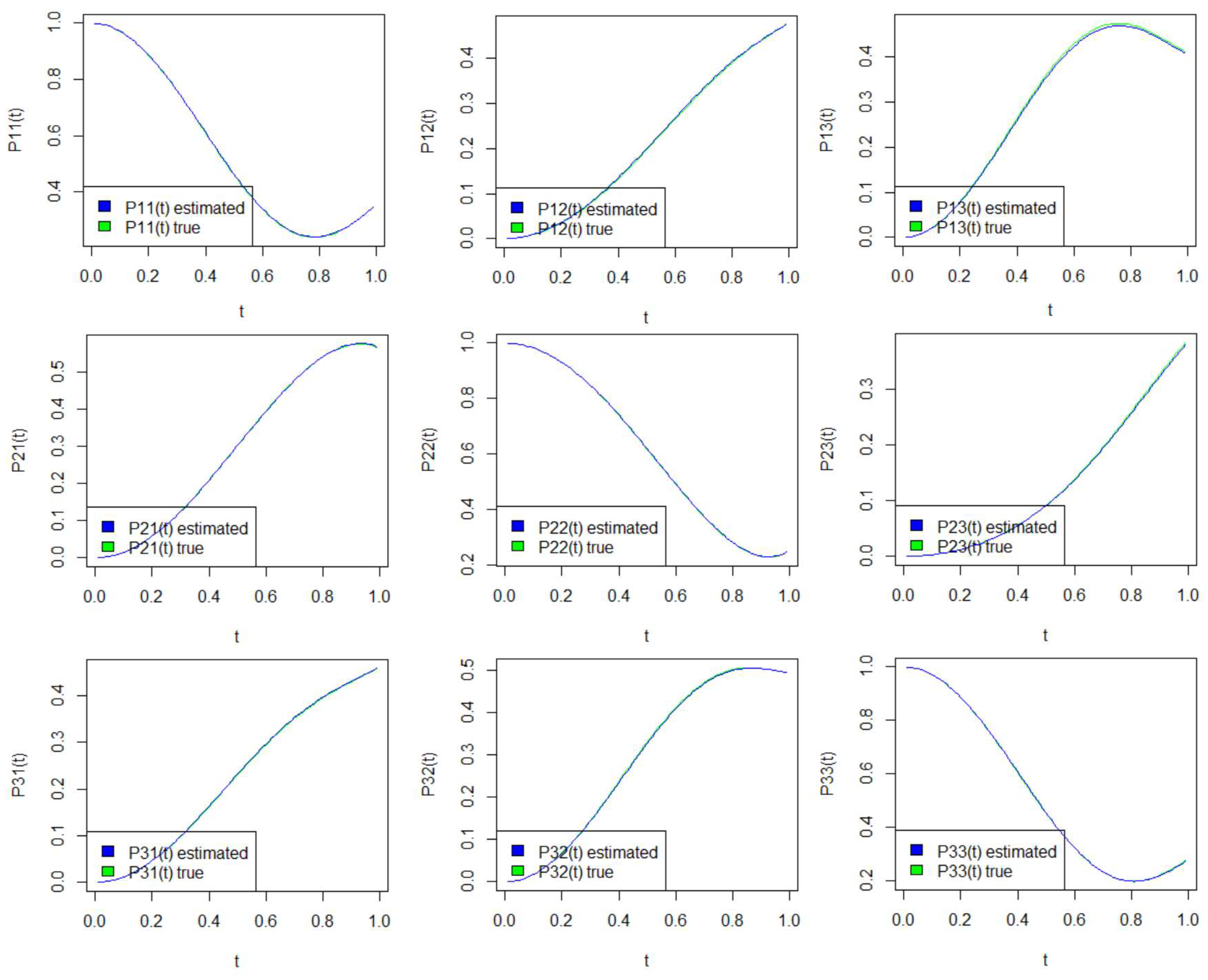
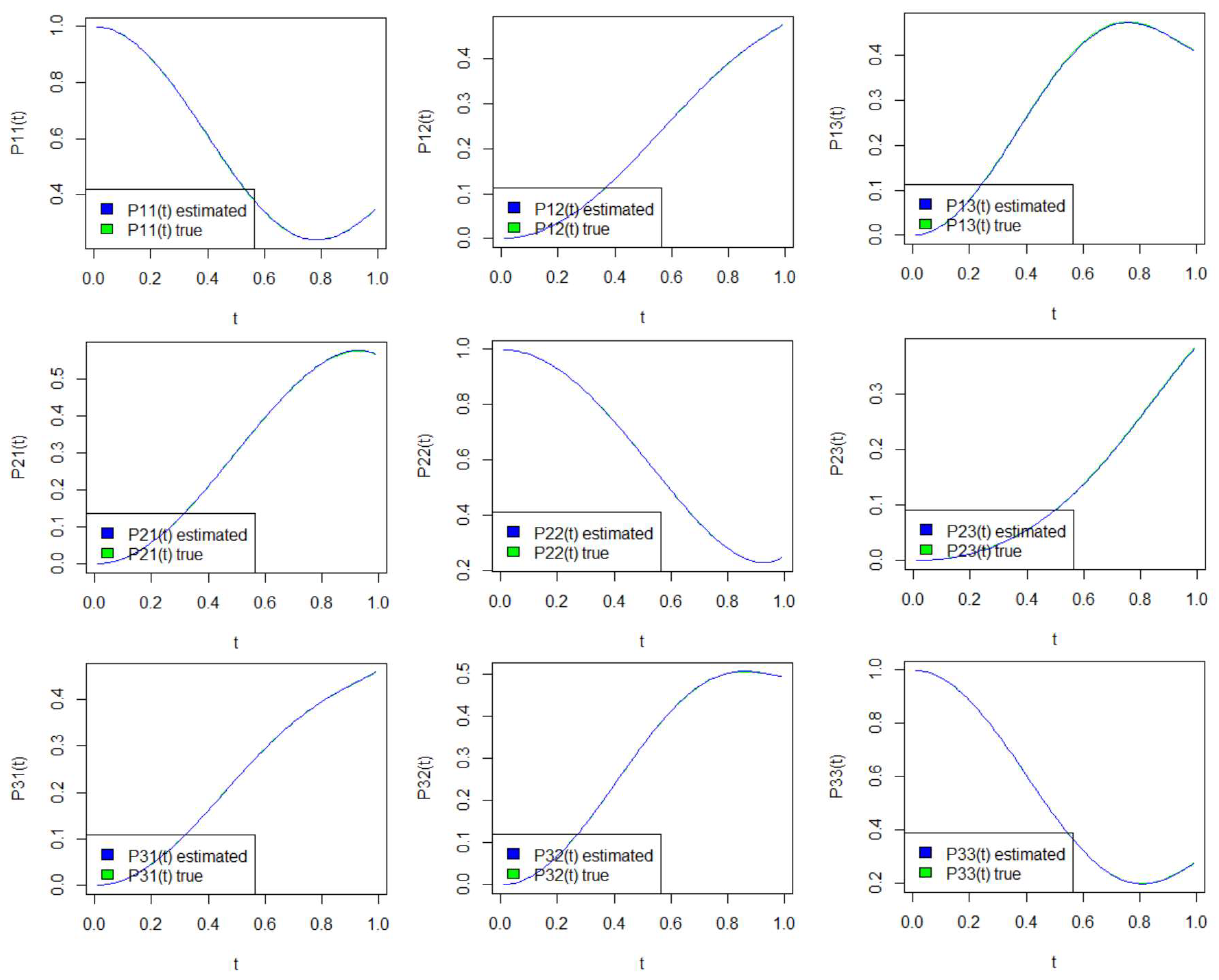
The results for the estimated transition probabilities of the semi-Markov process $P_{ij}\left(t\right)$ are provided in this subsection for various times t and for several sample paths, together with the associated standard errors.

Table 3. The estimated values of the initial law $a_i$ in the case of $L=1000$ trajectories without censoring.

i	1	2	3
${\widehat{\alpha }}_i(L,M)$	0.319	0.355	0.326

,

Table 4. Squared errors (S.E.) for the estimators of $a_{ij}$ and $p_{ij}$ in the case of no censoring, for various values of L.

L	5	10	100	1000
S.E.$\left({\widehat{a}}_{ij}(L,M)\right)$	$5.71\times {10}^{-3}$	$1.05\times {10}^{-3}$	$7\times {10}^{-4}$	$4.35\times {10}^{-5}$
S.E.$\left({\widehat{p}}_{ij}(L,M)\right)$	$2.6\times {10}^{-4}$	$1.06\times {10}^{-4}$	$1.47\times {10}^{-5}$	$7.58\times {10}^{-7}$

and

Table 5. Squared errors (S.E.) for the estimators of the semi-Markov transition probabilities in the case of no censoring.

t	0.1	0.2	0.5	0.9
S.E.$\left({\widehat{P}}_{ij}(t;L,M)\right)$	$2.72\times {10}^{-6}$	$3.75\times {10}^{-5}$	$4.47\times {10}^{-4}$	$1.34\times {10}^{-4}$

and Figure 1 refer to the uncensored case, while

Table 6. The estimated values of the initial law $a_i$ in the case of $L=1000$ trajectories with censoring at the beginning and/or at the end.

i	1	2	3
${\widehat{\alpha }}_i(L,M)$	0.328	0.328	0.344

,

Table 7. Squared errors (S.E.) for the estimators of $a_{ij}$ and $p_{ij}$ in the case of censoring at the beginning and/or at the end, for various values of L.

L	5	10	100	1000
S.E.$\left({\widehat{a}}_{ij}(L,M)\right)$	$1.13\times {10}^{-2}$	$6.18\times {10}^{-3}$	$2.79\times {10}^{-4}$	$3.27\times {10}^{-5}$
S.E.$\left({\widehat{p}}_{ij}(L,M)\right)$	$2\times {10}^{-4}$	$9.24\times {10}^{-5}$	$1.13\times {10}^{-5}$	$6.91\times {10}^{-7}$

and

Table 8. Squared errors for the estimators of the semi-Markov transition probabilities in the case of censoring at the beginning and/or at the end.

t	0.1	0.2	0.5	0.9
S.E.$\left({\widehat{P}}_{ij}(t;L,M)\right)$	$1.69\times {10}^{-6}$	$2.39\times {10}^{-5}$	$3.91\times {10}^{-4}$	$5.37\times {10}^{-4}$

and Figure 2 refer to the censored case.

According to the results in Table 4 and Table 7, the estimators are more accurate as the number of trajectories is increasing. Furthermore, the estimator of the initial law (Table 3 and Table 6) seems to be very close to the target value for both the censored and the uncensored case.

According to the above results, observe that as long as the time is close to the lower limit of the domain (i.e., close to 0), it is more likely that the process will remain in the same state (see

Table 9. Estimators for the transition probabilities of the semi-Markov process for $t=0.1$ and $t=0.5$.

${\widehat{\mathit{P}}}_{\mathit{i}\mathit{j}}(\mathit{t}=0.1)$	1	2	3	${\widehat{\mathit{P}}}_{\mathit{i}\mathit{j}}(\mathit{t}=0.5)$	1	2	3
1	0.970	0.009	0.021	1	0.456	0.200	0.358
2	0.014	0.983	0.003	2	0.288	0.625	0.096
3	0.012	0.017	0.971	3	0.226	0.326	0.460

and

Table 10. Estimators for the transition probabilities of the semi-Markov process for $t=0.7$ and $t=0.99$.

${\widehat{\mathit{P}}}_{\mathit{i}\mathit{j}}(\mathit{t}=0.7)$	1	2	3	${\widehat{\mathit{P}}}_{\mathit{i}\mathit{j}}(\mathit{t}=0.99)$	1	2	3
1	0.254	0.334	0.470	1	0.276	0.387	0.337
2	0.459	0.383	0.202	2	0.466	0.207	0.327
3	0.345	0.470	0.239	3	0.365	0.408	0.227

and Figure 1 and Figure 2). However, as time goes on, this changes. More specifically, for $t=0.7$, if the semi-Markov process is in state 1 at time 0, the most probable transition is to state 3. If the semi-Markov process starts at time 0 from state 2, the most probable transition is to state 1. If starting from state 3, the most probable transition is to state 2. For $t=0.99$, the semi-Markov process will most likely transition to state 2, given that at time 0, it has started in state 1 or 3. Finally, if it was in state 2, the process would most likely move to state 1. For the overall behavior of the estimators of the transition probabilities, see Table 5 and Table 8, where the associated standard errors are provided.

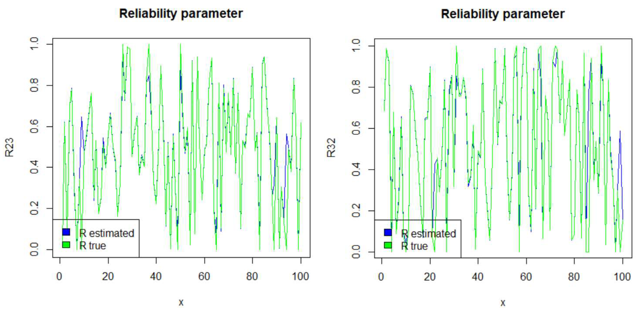
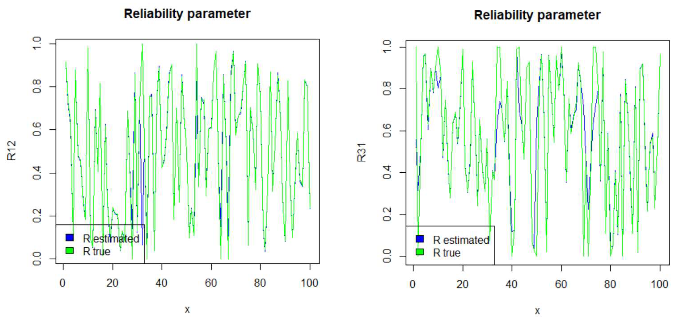
6.3. Reliability Parameter Estimation

In engineering, one of the main problems of interest is the event that the system remains in a working state during the whole observation period. As mentioned in the introduction, the performance of a system in mechanical engineering is evaluated via the reliability parameter. Such a system stays in a functioning condition as long as the stress (pressure) Y is at a lower level than the strength X. In general, in a multi-state system, the transition from one state to another may be defined according to whether a component of the system fails due to the fact that the stress exceeds the strength. In this section, we provide the performance of the estimator of the reliability parameter when X and Y follow the Kumaraswamy distribution with shape parameters $a_1$ and $a_2$, respectively. Observe that in Figure 3 and Figure 4, the estimated values (in blue) almost coincide with the true values (in green). We provide here the simulated results of the reliability parameter, using, for illustrative purposes, selected states i and j from the previous section. The notation $R_{ij}$ refers to the reliability parameter for i and j.

References

- Kumaraswamy, P. A generalized probability density function for double-bounded random processes. J. Hydrol. 1980, 46, 79–88. [Google Scholar] [CrossRef]
- Jones, M.C. Kumaraswamy’s distribution: A beta-type distribution with some tractability advantages. Stat. Methodol. 2008, 6, 70–81. [Google Scholar] [CrossRef]
- Kohansal, A. On estimation of reliability in a multicomponent stress-strength model for a Kumaraswamy distribution based on progressively censored sample. Stat. Pap. 2019, 60, 2185–2224. [Google Scholar] [CrossRef]
- Mitnik, P.A. New Properties of the Kumaraswamy Distribution. Comm. Stat. Theory Methods 2013, 42, 741–755. [Google Scholar] [CrossRef]
- Fletcher, S.G.; Ponnambalam, K. Estimation of reservoir yield and storage distribution using moments analysis. J. Hydrol. 1996, 182, 259–275. [Google Scholar] [CrossRef]
- Ganji, A.; Ponnambalam, K.; Khalili, D.; Karamouz, M. Grain yield reliability analysis with crop water demand uncertainty. Stoch. Environ. Res. Risk Assess. 2006, 2, 259–277. [Google Scholar] [CrossRef]
- Nadar, M.; Papadopoulos, A.; Kizilaslan, F. Statistical analysis for Kumaraswamy’s distribution based on record data. Stat. Pap. 2013, 54, 355–369. [Google Scholar] [CrossRef]
- Courard-Hauri, D. Using Monte Carlo analysis to investigate the relationship between overconsumption and uncertain access to one’s personal utility function. Ecol. Econ. 2007, 64, 152–162. [Google Scholar] [CrossRef]
- Seifi, A.; Ponnambalam, K.; Vlach, J. Maximization of manufacturing yield of systems with arbitrary distributions of component values. Ann. Oper. Res. 2000, 99, 373–383. [Google Scholar] [CrossRef]
- Cordeiro, G.M.; Edwin, M.M.; Ortega, S.N. The Kumaraswamy Weibull distribution with application to failure data. J. Franklin Inst. 2010, 347, 1399–1429. [Google Scholar] [CrossRef]
- Ghosh, I. On the reliability for some bivariate dependent Beta and Kumaraswamy distributions: A brief survey. Stoch. Qual. Control 2019, 34, 115–121. [Google Scholar] [CrossRef]
- Gilchrist, W.G. Statistical Modelling with Quantile Functions; Chapman & Hall/CRC: Boca Raton, FL, USA, 2001. [Google Scholar]
- Mitnik, P.A.; Baek, S. The Kumaraswamy distribution: Median-dispersion re-parameterizations for regression modeling and simulation-based estimation. Stat. Pap. 2013, 54, 177–192. [Google Scholar] [CrossRef]
- Cordeiro, G.M.; Castro, M. A new family of generalized distributions. J. Stat. Comput. Simul. 2011, 81, 883–898. [Google Scholar] [CrossRef]
- Eugene, N.; Lee, C.; Famoye, F. Beta-normal distribution and its applications. Comm. Stat. Theory Methods 2002, 31, 497–512. [Google Scholar] [CrossRef]
- Jones, M.C. Families of distributions arising from distributions of order statistics (with discussion). Test 2004, 13, 1–43. [Google Scholar] [CrossRef]
- Awad, A.M.; Azzam, M.M.; Hamdan, M.A. Some inference results on Pr(X < Y) in the bivariate exponential model. Comm. Stat. Theory Methods 1981, 10, 2515–2524. [Google Scholar]
- Church, J.D.; Harris, B. The estimation of reliability from stress strength relationships. Technometrics 1970, 12, 49–54. [Google Scholar] [CrossRef]
- Constantine, K.; Karson, M. Estimation of P(Y < X) in gamma case. Comm. Stat. Simul. Comput. 1986, 15, 365–388. [Google Scholar]
- Kotz, S.; Lumelskii, Y.; Pensky, M. The Stress-Strength Model and Its Generalizations. Theory and Applications; World Scientific: Singapore, 2003. [Google Scholar]
- Weerahandi, S.; Johnson, R.A. Testing reliability in a stress-strength model when X and Y are normally distributed. Technometrics 1992, 34, 83–91. [Google Scholar] [CrossRef]
- Balasubramanian, K.; Beg, M.I.; Bapat, R.B. On families of distributions closed under extrema. Sankhya A 1991, 53, 375–388. [Google Scholar]
- Barbu, V.S.; Karagrigoriou, A.; Makrides, A. Semi-Markov Modelling for Multi-State Systems. Methodol. Comput. Appl. Probab. 2017, 19, 1011–1028. [Google Scholar] [CrossRef]
- Slud, E.V.; Vonta, F. Efficient semiparametric estimators via modified profile likelihood. J. Stat. Plan. Inference 2005, 129, 339–367. [Google Scholar] [CrossRef]
- Asanjarani, A.; Liquet, B.; Nazarathy, Y. Estimation of semi-Markov multi-state models: A comparison of the sojourn times and transition intensities approaches. Int. J. Biostat. 2020. [Google Scholar] [CrossRef]
- Barbu, V.; Boussemart, M.; Limnios, N. Discrete-time semi-Markov model for reliability and survival analysis. Comm. Stat. Theory Methods 2004, 33, 2833–2868. [Google Scholar] [CrossRef]
- D’Amico, G.; Manca, R.; Petroni, F.; Selvamuthu, D. On the Computation of Some Interval Reliability Indicators for Semi-Markov Systems. Mathematics 2021, 9, 575. [Google Scholar] [CrossRef]
- Janssen, J.; Manca, R. Semi-Markov Risk Models for Finance, Insurance and Reliability; Springer: New York, NY, USA, 2007. [Google Scholar]
- Limnios, N.; Oprişan, G. Semi-Markov Processes and Reliability; Birkhäuser: Boston, MA, USA, 2001. [Google Scholar]
- Lisnianski, A.; Frenkel, I.; Karagrigoriou, A. Recent Advances in Multi-State Reliability, Theory and Applications; Springer Series in Reliability Engineering; Springer: Berlin, Germany, 2018. [Google Scholar]
- Lisnianski, A.; Levitin, G. Multi-State System Reliability: Assessment, Optimization and Applications; World Scientific: Singapore, 2003. [Google Scholar]
- Ouhbi, B.; Limnios, N. Non-parametric estimation for semi-Markov kernels with application to reliability analysis. Appl. Stoch. Models Data Anal. 1996, 12, 209–220. [Google Scholar] [CrossRef]
Figure 1.
Real and estimated semi-Markov transition probabilities in the case of uncensored trajectories.
Figure 2.
Real and estimated semi-Markov transition probabilities in the case of censored trajectories.
Figure 3.
Reliability parameters for the case of uncensored trajectories.
Figure 4.
Reliability parameters for the case of censoring at the beginning and/or at the end.