A New Nonlinear Ninth-Order Root-Finding Method with Error Analysis and Basins of Attraction

Abstract

Nonlinear phenomena occur in various fields of science, business, and engineering. Research in the area of computational science is constantly growing, with the development of new numerical schemes or with the modification of existing ones. However, such numerical schemes, objectively need to be computationally inexpensive with a higher order of convergence. Taking into account these demanding features, this article attempted to develop a new three-step numerical scheme to solve nonlinear scalar and vector equations. The scheme was shown to have ninth order convergence and requires six function evaluations per iteration. The efficiency index is approximately 1.4422, which is higher than the Newton’s scheme and several other known optimal schemes. Its dependence on the initial estimates was studied by using real multidimensional dynamical schemes, showing its stable behavior when tested upon some nonlinear models. Based on absolute errors, the number of iterations, the number of function evaluations, preassigned tolerance, convergence speed, and CPU time (sec), comparisons with well-known optimal schemes available in the literature showed a better performance of the proposed scheme. Practical models under consideration include open-channel flow in civil engineering, Planck’s radiation law in physics, the van der Waals equation in chemistry, and the steady-state of the Lorenz system in meteorology.

1. Introduction

Applied mathematics, biological sciences, and engineering disciplines are full of systems and processes whose response is not proportional to the input, thereby demanding numerical schemes with a high order of convergence and a reasonable computational cost. The literature has provided us with various numerical schemes to fulfill this demand, while still leaving significant room for continuous improvements in this vibrant area of numerical analysis. Fortunately, the need to solve nonlinear equations does not end with mathematical studies since many ordinary, partial, integral, and integro-differential equations often give rise to systems of nonlinear equations after discretization, so they must be handled with numerical schemes. Generally, nonlinear phenomena designed in terms of models with nonlinear equations are seen not only in academia and the physical industry, but also in the fields of medical sciences and other real-world situations. For instance, the triangulation of GPS signals, combustion, heat transfer, and fluid flow amongst others are some of those fields [1,2,3,4].

When it comes to solving nonlinear equations arising from physical and natural sciences, researchers often resort to numerical schemes as such equations are, in many cases, extremely complicated to be solved to obtain the exact solutions. Because of this, mathematicians, mostly those working in applied fields, are trying to obtain numerical schemes with higher orders of convergence, but at the same time, with a reduced number of function evaluations required for each iteration, while keeping in mind the importance of the stability features of the schemes. Among various existing classical schemes, Newton–Raphson (NR) is always considered the first choice due to its simplicity. Like the Euler scheme in ordinary differential equations, the NR scheme serves as a basic building block for the emergence of many higher-order numerical schemes to solve nonlinear equations. Since achieving an optimal order of convergence is not always possible, because of Kung and Traub’s conjecture [5], several researchers have primarily focused on achieving a high order of convergence with a low number of function evaluations per iteration. In this context, we cannot ignore the concept of efficiency index (E) defined as $E=p^{1/c}$, where p and c are the convergence order and the number of function evaluations required at each step, respectively. Some notable recently developed nonlinear schemes include the homotopy perturbation method [6,7], the Adomian decomposition method [8], the variational iteration method [9,10], and those based on quadrature rules [11,12].

In [13], the authors combined two schemes of orders $p_1$ and $p_2$ to design a new two-step scheme with order $p_1{p}_2$. The process brings additional function evaluations at each step of the iteration, however, with a higher order of convergence. On the other hand, Noor and Noor [14] developed a three-step scheme with third-order convergence at the cost of five function evaluations per iteration and Noor et al. [15] presented two schemes having third- and fourth-order convergence needing five and eight function evaluations per iteration, respectively. Consequently, Shah et al. [16] proposed a three-step sixth-order convergent scheme that uses seven function evaluations per iteration. Such approaches, despite being convergent with high orders, require additional computational cost in terms of CPU time. A recently published study [17] used a similar approach to obtain an efficient three-step numerical scheme. The main objective of this research was to develop a new hybrid three-step numerical scheme to solve both scalar and vector nonlinear equations. Motivated by such approaches, we attempted to develop a new three-step numerical scheme by combining a modified third-order Newton scheme in [18] with the classical third-order Halley scheme [19]. This resulted in a ninth-order scheme which only needs six function evaluations—three functions, two first-order derivatives, and one second-order derivative–per iteration. The new scheme is advantageous in terms of absolute errors, number of function evaluations, number of iterations required to achieve a pre-assigned accuracy, computational time, and efficiency index, compared to some available schemes.

This paper is structured as follows. Section 2 presents information about some existing schemes. Then, the formulation of the proposed scheme and the derivation of its order of convergence and asymptotic error terms in both cases of scalar and vector equations follow. Some theoretical comparisons are addressed with a stability analysis and basins of attraction of the proposed scheme. Some numerical experiments containing applied problems are presented in Section 3. Finally, Section 4 brings the paper to an end with a discussion of major findings and future research directions.

2. Previous Materials and Methods

In this section, we will briefly review some well-known numerical schemes that are frequently used to determine approximate solutions to nonlinear models. Indeed, when it comes to solving such nonlinear models, there is objectively no analytical technique to yield exact results. Thus, we are obliged to use numerical schemes.

2.1. Brief Overview of Some Existing Schemes

When someone thinks of solving a nonlinear equation with a numerical scheme, the first scheme that comes to mind is the classical Newton–Raphson [5] which has optimal second-order convergence. In short, we used the symbol NR2 for this scheme which uses two function evaluations—one function and one first-order derivative—per iteration. The scheme is given by

$$x_{n+1}=x_n-{\displaystyle \frac{f\left(x_n\right)}{f^{\prime }\left(x_n\right)}},n=0,1,2,\dots .$$

(1)

In [20], one can find the classical third-order Halley’s numerical scheme (denoted by Halley3). This scheme needs three function evaluations (one function, one first-order derivative and one second-order derivative) per iteration and is given by

$$x_{n+1}=x_n-{\displaystyle \frac{2f\left(x_n\right)f^{\prime }\left(x_n\right)}{2{\left(f^{\prime }\left(x_n\right)\right)}^2-f\left(x_n\right)f^{″}\left(x_n\right)}},n=0,1,2,\dots .$$

(2)

By using NR2 (1) as a predictor, Halley’s as corrector, and the finite difference approximation of the second derivative, a new numerical scheme was suggested in [21] named the modified Halley method (MHM5). It possesses fifth-order convergence and needs four function evaluations (two function and two first-order derivatives) per iteration. The scheme is given by

$$\begin{array}{c}\hfill \begin{array}{cc}\hfill y_n& =x_n-{\displaystyle \frac{f\left(x_n\right)}{f^{\prime }\left(x_n\right)}},\hfill \\ \hfill x_{n+1}& =y_n-{\displaystyle \frac{2f\left(x_n\right)f\left(y_n\right)f^{\prime }\left(y_n\right)}{2f\left(x_n\right)f^{\prime 2}\left(y_n\right)-f^{\prime 2}\left(x_n\right)f\left(y_n\right)+f^{\prime }\left(x_n\right)f\left(y_n\right)f^{\prime }\left(y_n\right)}},\hfill \end{array}\end{array}\} \begin{array}{c}n=0,1,2,\dots .\hfill \end{array}$$

(3)

With the use of five function evaluations (three function, and two first-order derivatives), a three-step numerical scheme was discussed in [22] whose theoretical order of convergence, as proved by the authors, is 9. The scheme is given by

$$\begin{array}{c}\hfill \begin{array}{cc}\hfill y_n& =x_n-{\displaystyle \frac{f\left(x_n\right)}{f^{\prime }\left(x_n\right)}},\hfill \\ \hfill z_n& =y_n-{\displaystyle \frac{(x_n-y_n)f\left(y_n\right)}{f\left(x_n\right)-2f\left(y_n\right)}},\hfill \\ \hfill x_{n+1}& =z_n-{\displaystyle \frac{f\left(z_n\right)f^{\prime }\left(z_n\right)}{f^{\prime 2}\left(z_n\right)-2\lambda f\left(z_n\right){\displaystyle \frac{f\left(z_n\right)-f\left(x_n\right)-f^{\prime }\left(x_n\right)(z_n-x_n)}{{(z_n-x_n)}^2}}}},\lambda =\frac{1}{2}.\hfill \end{array}\end{array}\} \begin{array}{c}n=0,1,2,\dots .\hfill \end{array}$$

(4)

A two-step numerical scheme of order nine proposed in [23] uses seven function evaluations per iteration (two function, two first-order derivatives, two second-order derivatives and one third-order derivative). The scheme is given by

$$\begin{array}{c}\hfill \begin{array}{cc}\hfill y_n& =x_n-{\displaystyle \frac{f\left(x_n\right)}{f^{\prime }\left(x_n\right)}}-{\displaystyle \frac{f^2\left(x_n\right)f^{″}\left(x_n\right)}{2f^{\prime 3}\left(x_n\right)}},\hfill \\ \hfill x_{n+1}& =y_n-{\displaystyle \frac{f\left(y_n\right)}{f^{\prime }\left(y_n\right)}}-{\displaystyle \frac{f^2\left(y_n\right)f^{″}\left(y_n\right)}{2f^{\prime 3}\left(y_n\right)}}-{\displaystyle \frac{f^3\left(y_n\right)f^{‴}\left(y_n\right)}{6f^{\prime 4}\left(y_n\right)}}.\hfill \end{array}\end{array}\} \begin{array}{c}n=0,1,2,\dots .\hfill \end{array}$$

(5)

Most recently, the authors in [24] devised, using a variational iteration approach, a new three-step numerical scheme to solve nonlinear scalar equations. Their proposed scheme is ninth-order convergent with six function evaluations (three function, two first-order derivatives and one second-order derivative) per iteration. The scheme is as follows:

$$\begin{array}{c}\hfill \begin{array}{cc}\hfill y_n& =x_n-{\displaystyle \frac{f\left(x_n\right)}{f^{\prime }\left(x_n\right)}}-{\displaystyle \frac{f^2\left(x_n\right)f^{″}\left(x_n\right)}{2f^{\prime 3}\left(x_n\right)}},\hfill \\ \hfill z_n& =y_n-{\displaystyle \frac{f\left(y_n\right)}{f^{\prime }\left(y_n\right)}},\hfill \\ \hfill x_{n+1}& =z_n-{\displaystyle \frac{f\left(z_n\right)}{f^{\prime }\left(y_n\right)-\beta f\left(y_n\right)}},\beta =1.\hfill \end{array}\end{array}\} \begin{array}{c}n=0,1,2,\dots .\hfill \end{array}$$

(6)

The numerical schemes discussed above will be used for comparison purposes in the present study.

2.2. Proposed Numerical Scheme

After the thorough investigation of the existing literature, we observed that several authors have proposed new hybrid type schemes using the second-order NR scheme as their starting step, aiming to increase the order of convergence and reduce the number of function evaluations. However, we took a step forward to use the third-order Halley’s scheme in the first step:

$$x_{n+1}=x_n-\frac{2f\left(x_n\right)f^{\prime }\left(x_n\right)}{2f^{\prime }{\left(x_n\right)}^2-f\left(x_n\right)f^{″}\left(x_n\right)},$$

(7)

to be blended with the third-order modified Newton scheme given below:

$$\begin{array}{cc}\hfill & y_n=x_n-\frac{f\left(x_n\right)}{f^{\prime }\left(x_n\right)},\hfill \\ \hfill & x_{n+1}=x_n-\frac{f\left(x_n\right)+f\left(y_n\right)}{f^{\prime }\left(x_n\right)}.\hfill \end{array}$$

(8)

The aim was to obtain a new nonlinear scheme with a higher order of convergence while the number of function evaluations per iteration was reduced as much as possible. Such an idea was carried out in [13] and later used by many authors. Hence, after blending both schemes above (7) and (8), we obtain the following new nonlinear scheme:

$$\begin{array}{cc}\hfill & y_n=x_n-\frac{2f\left(x_n\right)f^{\prime }\left(x_n\right)}{2f^{\prime }{\left(x_n\right)}^2-f\left(x_n\right)f^{″}\left(x_n\right)},\hfill \\ \hfill & z_n=y_n-\frac{f\left(y_n\right)}{f^{\prime }\left(y_n\right)},\hfill \\ \hfill & x_{n+1}=y_n-\frac{f\left(y_n\right)+f\left(z_n\right)}{f^{\prime }\left(y_n\right)}.\hfill \end{array}$$

(9)

The proposed scheme will be referred to as PS9 for the rest of the paper, wherein its theoretical analysis, including convergence theory, stability, and bifurcation phenomenon are discussed in detail.

2.2.1. Convergence Analysis for $f\left(x\right)=0$

In the following theorem, we prove the ninth-order of convergence for the proposed nonlinear three-step scheme given in (9).

Theorem 1.

Let γ be the root of a sufficiently differentiable function $f:\Pi \subset \mathbb{R}\to \mathbb{R}$ on an open interval Π. Then, the three-step scheme PS9 presented in (9) has ninth-order convergence, and the error equation is:

$${\epsilon }_{j+1}=A{\epsilon }_j^9+\mathcal{O}({\epsilon }_j^{10}),$$

(10)

where $A={\displaystyle \frac{1}{128}}{\left({\displaystyle \frac{f^{″}\left(\gamma \right)}{f^{\prime }\left(\gamma \right)}}\right)}^8$ and ${\epsilon }_j=x_j-\gamma$.

Proof. 

Let $\gamma$ be the root of $f\left(x\right)=0$, $x_j$ be the jth approximation to the root provided by PS9 and ${\epsilon }_j=x_j-\gamma$ be the error term after the jth iteration. Using Taylor’s expansion for $f\left(x_j\right)$ about $\gamma$, we have:

$$f\left(x_j\right)=f^{\prime }\left(\gamma \right){\epsilon }_j+{\displaystyle \frac{1}{2}}{f}^{″}\left(\gamma \right){\epsilon }_j^2+\mathcal{O}({\epsilon }_j^3).$$

(11)

Expanding $f^{\prime }\left(x_j\right)$ via Taylor’s series about $\gamma$, we have:

$$f^{\prime }\left(x_j\right)=f^{\prime }\left(\gamma \right)+f^{″}\left(\gamma \right){\epsilon }_j+{\displaystyle \frac{1}{2}}{f}^{‴}\left(\gamma \right){\epsilon }_j^2+\mathcal{O}({\epsilon }_j^3).$$

(12)

Multiplying (11) and (12), we obtain:

$$f\left(x_j\right)f^{\prime }\left(x_j\right)=f^{\prime 2}\left(\gamma \right){\epsilon }_j+{\displaystyle \frac{3}{2}}{f}^{\prime }\left(\gamma \right)f^{″}\left(\gamma \right){\epsilon }_j^2+{\displaystyle \frac{1}{2}}\left(f^{\prime }\left(\gamma \right)f^{‴}\left(\gamma \right)+f^{″2}\left(\gamma \right)\right){\epsilon }_j^3+\mathcal{O}({\epsilon }_j^4).$$

(13)

Now, the Taylor expansion of the denominator in the fractional term in the first step of (9) multiplied by its numerator results in:

$$\frac{2f\left(x_j\right)f^{\prime }\left(x_j\right)}{2f^{\prime }{\left(x_j\right)}^2-f\left(x_j\right)f^{″}\left(x_j\right)}={\epsilon }_j-{\displaystyle \frac{1}{4f^{\prime 2}\left(\gamma \right)}}{f}^{″2}\left(\gamma \right){\epsilon }_j^3-{\displaystyle \frac{1}{4f^{\prime 3}\left(\gamma \right)}}{f}^{″}\left(\gamma \right)\left(5f^{\prime }\left(\gamma \right)f^{‴}\left(\gamma \right)-6f^{″2}\left(\gamma \right)\right){\epsilon }_j^4+\mathcal{O}({\epsilon }_j^5).$$

(14)

Using (14) in the first step of (9), we obtain:

$${\zeta }_j=y_j-\gamma ={\displaystyle \frac{1}{4f^{\prime 2}\left(\gamma \right)}}{f}^{″2}\left(\gamma \right){\epsilon }_j^3+{\displaystyle \frac{1}{4f^{\prime 3}\left(\gamma \right)}}{f}^{″}\left(\gamma \right)\left(5f^{\prime }\left(\gamma \right)f^{‴}\left(\gamma \right)-6f^{″2}\left(\gamma \right)\right){\epsilon }_j^4+\mathcal{O}({\epsilon }_j^5).$$

(15)

Using Taylor’s expansion for $f\left(y_j\right)$ about $\gamma$, we have:

$$f\left(y_j\right)=f^{\prime }\left(\gamma \right){\zeta }_j+{\displaystyle \frac{1}{2}}{f}^{″}\left(\gamma \right){\zeta }_j^2+\mathcal{O}({\zeta }_j^3).$$

(16)

Using the Taylor’s expansion for $1/f^{\prime }\left(y_j\right)$ about $\gamma$, we have

$$\frac{1}{f^{\prime }\left(y_j\right)}=\frac{1}{f^{\prime }\left(\gamma \right)}-\frac{f^{″}\left(\gamma \right)}{f^{\prime 2}\left(\gamma \right)}{\zeta }_j+{\displaystyle \frac{1}{f^{\prime }\left(\gamma \right)}}\left(-{\displaystyle \frac{f^{‴}\left(\gamma \right)}{2f^{\prime }\left(\gamma \right)}}+{\displaystyle \frac{f^{″2}\left(\gamma \right)}{f^{\prime 2}\left(\gamma \right)}}\right){\zeta }_j^2+\mathcal{O}({\zeta }_j^3).$$

(17)

Multiplying (16) by (17), we obtain:

$$\frac{f\left(y_j\right)}{f^{\prime }\left(y_j\right)}={\zeta }_j-\frac{f^{″}\left(\gamma \right)}{2f^{\prime }\left(\gamma \right)}{\zeta }_j^2-{\displaystyle \frac{f^{\prime }\left(\gamma \right)f^{‴}\left(\gamma \right)-f^{″2}\left(\gamma \right)}{2f^{\prime 2}\left(\gamma \right)}}{\zeta }_j^3+\mathcal{O}({\zeta }_j^4).$$

(18)

Using (18) in the second step of (9), we have:

$${\nu }_j=z_j-\gamma =\frac{f^{″}\left(\gamma \right)}{2f^{\prime }\left(\gamma \right)}{\zeta }_j^2+{\displaystyle \frac{f^{\prime }\left(\gamma \right)f^{‴}\left(\gamma \right)-f^{″2}\left(\gamma \right)}{2f^{\prime 2}\left(\gamma \right)}}{\zeta }_j^3+\mathcal{O}({\zeta }_j^4).$$

(19)

Now, using the Taylor expansion for $f\left(z_j\right)$ about $\gamma$, we have:

$$f\left(z_j\right)=f^{\prime }\left(\gamma \right){\nu }_j+\mathcal{O}({\nu }_j^2).$$

(20)

Using (16), (17), and (20) in the third step of (9), we have (note that, for brevity, we suppressed the $\gamma$ in the derivatives):

$${\epsilon }_{j+1}=-{\nu }_j+{\displaystyle \frac{f^{″}}{2f^{\prime }}}{\zeta }_j^2+{\displaystyle \frac{1}{2f^{\prime }}}\left(f^{‴}-{\displaystyle \frac{f^{″2}}{f^{\prime }}}\right){\zeta }_j^3+{\displaystyle \frac{f^{″}}{2f^{\prime 2}}}\left({\displaystyle \frac{f^{‴}}{2}}-{\displaystyle \frac{f^{″2}}{f^{\prime }}}\right){\zeta }_j^4+{\displaystyle \frac{f^{″}}{f^{\prime }}}{\zeta }_j{\nu }_j+{\displaystyle \frac{1}{f^{\prime }}}\left(f^{‴}-{\displaystyle \frac{f^{″2}}{f^{\prime }}}\right){\zeta }_j^2{\nu }_j+\mathcal{O}({\epsilon }_j^{10}).$$

(21)

Using (19) in (21), we have:

$${\epsilon }_{j+1}={\displaystyle \frac{1}{2}}{\left({\displaystyle \frac{f^{″}}{f^{\prime }}}\right)}^2{\zeta }_j^3+{\displaystyle \frac{1}{4f^{\prime 3}}}{f}^{″}(3f^{\prime }{f}^{‴}-4f^{″2}){\zeta }_j^4+\mathcal{O}({\epsilon }_j^{10}).$$

(22)

Finally, using (15) in (22), we obtain:

$${\epsilon }_{j+1}={\displaystyle \frac{1}{128}}{\left({\displaystyle \frac{f^{″}\left(\gamma \right)}{f^{\prime }\left(\gamma \right)}}\right)}^8{\epsilon }_j^9+\mathcal{O}({\epsilon }_j^{10}),$$

(23)

which proves the ninth-order convergence of the proposed scheme PS9 in (9). □

2.2.2. Convergence Analysis for $\mathit{F}\left(\mathit{x}\right)=\mathbf{0}$

Now, let us consider a nonlinear system of N equations and N variables, $\mathit{F}\left(\mathit{x}\right)=\mathbf{0}$, where $\mathit{F}:\Pi \subset {\mathbb{R}}^N\to {\mathbb{R}}^N$ is a sufficiently Frechet differentiable function. In this case, the PS9 method adopts the form:

$$\begin{array}{cc}\hfill & {\mathit{y}}_n={\mathit{x}}_n-{\left[2{\mathit{F}}^{\prime }{\left({\mathit{x}}_n\right)}^2-\mathit{F}\left({\mathit{x}}_n\right){\mathit{F}}^{″}\left({\mathit{x}}_n\right)\right]}^{-1}\left[2\mathit{F}\left({\mathit{x}}_n\right){\mathit{F}}^{\prime }\left({\mathit{x}}_n\right)\right],\hfill \\ \hfill & {\mathit{z}}_n={\mathit{y}}_n-{\mathit{F}}^{\prime }{\left({\mathit{y}}_n\right)}^{-1}\mathit{F}\left({\mathit{y}}_n\right),\hfill \\ \hfill & {\mathit{x}}_{n+1}={\mathit{y}}_n-{\mathit{F}}^{\prime }{\left({\mathit{y}}_n\right)}^{-1}\left[\mathit{F}\left({\mathit{y}}_n\right)+\mathit{F}\left({\mathit{z}}_n\right)\right],\hfill \end{array}$$

(24)

where ${\mathit{F}}^{\prime }$ is the Jacobian matrix of $\mathit{F}$.

We present the following results to show the error equation, and therefore, the order of convergence of the proposed scheme in the case of a system of nonlinear equations.

Lemma 1.

([17]). Let $\mathit{F}:\Pi \subset {\mathbb{R}}^N\to {\mathbb{R}}^N$ be an $r-$ times Frechet differentiable in a convex set $\Pi \subset {\mathbb{R}}^N$. Then, for any $\mathit{x}$ and $h\in {\mathbb{R}}^N$ the following expression holds

$$\mathit{F}(\mathit{x}+h)=\mathit{F}\left(\mathit{x}\right)+{\mathit{F}}^{\prime }\left(\mathit{x}\right)h+{\displaystyle \frac{1}{2!}}{\mathit{F}}^{″}\left(\mathit{x}\right)h^2+{\displaystyle \frac{1}{3!}}{\mathit{F}}^{‴}\left(\mathit{x}\right)h^3+\dots +{\displaystyle \frac{1}{(r-1)!}}{\mathit{F}}^{(r-1)}\left(\mathit{x}\right)h^{r-1}+R_r,$$

(25)

where $\left|\right|R_r\left|\right|\le \frac{1}{r!}\underset{0<t<1}{sup}\left|\right|{\mathit{F}}^{\left(r\right)}{(\mathit{x}+ht)\left|\right|\left|\right|h\left|\right|}^r$ and the notation ${\mathit{F}}^{\left(p\right)}\left(\mathit{x}\right)h^p$ stands for ${\mathit{F}}^{\left(p\right)}\left(\mathit{x}\right)h^p=(\cdots \left({\mathit{F}}^{\left(p\right)}\left(\mathit{x}\right)h\right)\stackrel{p}{\cdots })h\in {\mathbb{R}}^N$.

Theorem 2.

Let the function $\mathit{F}:\Pi \subset {\mathbb{R}}^N\to {\mathbb{R}}^N$ be sufficiently differentiable in a convex set Π containing a simple zero $\overrightarrow{\gamma }$ of $\mathit{F}\left(\mathit{x}\right)$. Let us consider that ${\mathit{F}}^{\prime }\left(\mathit{x}\right)$ is continuous and nonsingular in $\overrightarrow{\gamma }$. If the initial guess ${\mathit{x}}_0$ is close to $\overrightarrow{\gamma }$ then the sequence $\left\{{\mathit{x}}_j\right\}$ obtained with the proposed three-step scheme PS9 converges to $\overrightarrow{\gamma }$ with ninth-order convergence.

Proof. 

Let $\overrightarrow{\gamma }$ be the root of $\mathit{F}\left(\mathit{x}\right)$, ${\mathit{x}}_j$ be the jth approximation to the root by PS9 and ${\epsilon }_j={\mathit{x}}_j-\overrightarrow{\gamma }$ be the error vector after the jth iteration. Using Taylor’s expansion of $\mathit{F}\left({\mathit{x}}_j\right)$ about $\overrightarrow{\gamma }$, we have:

$$\mathit{F}\left({\mathit{x}}_j\right)={\mathit{F}}^{\prime }\left(\overrightarrow{\gamma }\right){\epsilon }_j+{\displaystyle \frac{1}{2}}{\mathit{F}}^{″}\left(\overrightarrow{\gamma }\right){\epsilon }_j^2+\mathcal{O}({\epsilon }_j^3).$$

(26)

Using Taylor’s expansion of ${\mathit{F}}^{\prime }\left({\mathit{x}}_j\right)$ about $\overrightarrow{\gamma }$, we have:

$${\mathit{F}}^{\prime }\left({\mathit{x}}_j\right)={\mathit{F}}^{\prime }\left(\overrightarrow{\gamma }\right)+{\mathit{F}}^{″}\left(\overrightarrow{\gamma }\right){\epsilon }_j+{\displaystyle \frac{1}{2}}{\mathit{F}}^{‴}\left(\overrightarrow{\gamma }\right){\epsilon }_j^2+\mathcal{O}({\epsilon }_j^3).$$

(27)

Multiplying (26) and (27), we obtain:

$$\mathit{F}\left({\mathit{x}}_j\right){\mathit{F}}^{\prime }\left({\mathit{x}}_j\right)={\mathit{F}}^{\prime 2}\left(\overrightarrow{\gamma }\right){\epsilon }_j+{\displaystyle \frac{3}{2}}{\mathit{F}}^{\prime }\left(\overrightarrow{\gamma }\right){\mathit{F}}^{″}\left(\overrightarrow{\gamma }\right){\epsilon }_j^2+{\displaystyle \frac{1}{2}}\left({\mathit{F}}^{\prime }(\overrightarrow{\gamma }){\mathit{F}}^{‴}(\overrightarrow{\gamma })+{\mathit{F}}^{″2}(\overrightarrow{\gamma })\right){\epsilon }_j^3+\mathcal{O}({\epsilon }_j^4).$$

(28)

Using Taylor’s expansion for the inverse matrix ${\left[2{\mathit{F}}^{\prime }{\left({\mathit{x}}_j\right)}^2-\mathit{F}\left({\mathit{x}}_j\right){\mathit{F}}^{″}\left({\mathit{x}}_j\right)\right]}^{-1}$ about $\overrightarrow{\gamma }$, we obtain:

$${\left[2{\mathit{F}}^{\prime }{\left({\mathit{x}}_j\right)}^2-\mathit{F}\left({\mathit{x}}_j\right){\mathit{F}}^{″}\left({\mathit{x}}_j\right)\right]}^{-1}={\displaystyle \frac{1}{2}}{\left[{\mathit{F}}^{\prime 2}(\overrightarrow{\gamma })\right]}^{-1}-{\displaystyle \frac{3}{4}}{\left[{\mathit{F}}^{\prime 3}\left(\overrightarrow{\gamma }\right)\right]}^{-1}{\mathit{F}}^{″}\left(\overrightarrow{\gamma }\right){\epsilon }_j+\mathcal{O}({\epsilon }_j^2).$$

(29)

Applying (29) to $2\mathit{F}\left({\mathit{x}}_j\right){\mathit{F}}^{\prime }\left({\mathit{x}}_j\right)$ after using (28), we have:

$$\begin{array}{cc}\hfill & {\left[2{\mathit{F}}^{\prime }{\left({\mathit{x}}_j\right)}^2-\mathit{F}\left({\mathit{x}}_j\right){\mathit{F}}^{″}\left({\mathit{x}}_j\right)\right]}^{-1}\left[2\mathit{F}\left({\mathit{x}}_j\right){\mathit{F}}^{\prime }\left({\mathit{x}}_j\right)\right]=\hfill \\ \hfill & {\epsilon }_j-{\displaystyle \frac{1}{4}}{\left[{\mathit{F}}^{\prime 2}(\overrightarrow{\gamma })\right]}^{-1}{\mathit{F}}^{″2}(\overrightarrow{\gamma }){\epsilon }_j^3-{\displaystyle \frac{1}{4}}{\left[{\mathit{F}}^{\prime 3}(\overrightarrow{\gamma })\right]}^{-1}{\mathit{F}}^{″}(\overrightarrow{\gamma })\left(5{\mathit{F}}^{\prime }(\overrightarrow{\gamma }){\mathit{F}}^{‴}(\overrightarrow{\gamma })-6{\mathit{F}}^{″2}(\overrightarrow{\gamma })\right){\epsilon }_j^4+\mathcal{O}({\epsilon }_j^5).\hfill \end{array}$$

(30)

Using (30) in the first step of (24), we obtain:

$${\zeta }_j=y_j-\overrightarrow{\gamma }={\displaystyle \frac{1}{4}}{\left[{\mathit{F}}^{\prime 2}(\overrightarrow{\gamma })\right]}^{-1}{\mathit{F}}^{″2}(\overrightarrow{\gamma }){\epsilon }_j^3+{\displaystyle \frac{1}{4}}{\left[{\mathit{F}}^{\prime 3}(\overrightarrow{\gamma })\right]}^{-1}{\mathit{F}}^{″}(\overrightarrow{\gamma })\left(5{\mathit{F}}^{\prime }(\overrightarrow{\gamma }){\mathit{F}}^{‴}(\overrightarrow{\gamma })-6{\mathit{F}}^{″2}(\overrightarrow{\gamma })\right){\epsilon }_j^4+\mathcal{O}({\epsilon }_j^5).$$

(31)

Likewise, using Taylor’s expansion for $\mathit{F}\left({\mathit{y}}_n\right)$ and ${\mathit{F}}^{\prime }\left({\mathit{x}}_n\right)$ about $\overrightarrow{\gamma }$; and ${\mathit{F}}^{\prime }\left({\mathit{y}}_n\right)$ in the second step of (24), we obtain:

$${\nu }_j={\mathbf{z}}_j-\overrightarrow{\gamma }={\displaystyle \frac{1}{2}}{\left[{\mathit{F}}^{\prime }(\overrightarrow{\gamma })\right]}^{-1}{\mathit{F}}^{″}(\overrightarrow{\gamma }){\zeta }_j^2+{\displaystyle \frac{1}{2}}{\left[{\mathit{F}}^{\prime 2}(\overrightarrow{\gamma })\right]}^{-1}\left({\mathit{F}}^{\prime }(\overrightarrow{\gamma }){\mathit{F}}^{‴}(\overrightarrow{\gamma })-{\mathit{F}}^{″2}(\overrightarrow{\gamma })\right){\zeta }_j^3+\mathcal{O}({\zeta }_j^4).$$

(32)

Finally, we use the Taylor series for $\mathit{F}\left({\mathit{z}}_n\right)$ about $\overrightarrow{\gamma }$ and earlier found series to obtain the following:

$${ϵ}_{j+1}={\displaystyle \frac{1}{2}}{\left[{\mathit{F}}^{\prime 2}(\overrightarrow{\gamma })\right]}^{-1}{\mathit{F}}^{″2}(\overrightarrow{\gamma }){\zeta }_j^3+{\displaystyle \frac{1}{4}}{\left[{\mathit{F}}^{\prime 3}(\overrightarrow{\gamma })\right]}^{-1}{\mathit{F}}^{″}(\overrightarrow{\gamma })\left(3{\mathit{F}}^{\prime }(\overrightarrow{\gamma }){\mathit{F}}^{‴}(\overrightarrow{\gamma })-4{\mathit{F}}^{″2}(\overrightarrow{\gamma })\right){\zeta }_j^4+\mathcal{O}({ϵ}_j^{10}).$$

(33)

Putting (31) in the above equation, we obtain the required result as follows:

$${ϵ}_{j+1}={\displaystyle \frac{1}{128}}{\mathit{F}}^{\prime 8}{(\overrightarrow{\gamma })}^{-1}{\mathit{F}}^{″8}(\overrightarrow{\gamma }){ϵ}_j^9+\mathcal{O}({ϵ}_j^{10}).$$

(34)

Hence, the ninth-order convergence of the proposed scheme PS9 has also been proven in the case of nonlinear systems. □

2.2.3. Numerical Comparison

A few numerical schemes were briefly introduced in Section 2.1, whose practical comparison can be made with the proposed scheme. The following abbreviations will be used hereinafter:

NR2	Newton–Raphson scheme with second-order convergence given in (1);
Halley3	Halley’s scheme with third-order convergence given in (2);
MHM5	Modified Halley’s scheme with fifth-order convergence given in (3);
HD9	A numerical scheme with ninth-order convergence given in (4);
NZ9	A numerical scheme with ninth-order convergence given in (5);
NA9	A numerical scheme with ninth-order convergence given in (6);
PS9	Proposed numerical scheme with ninth-order convergence given in (9);
FE	Number of function evaluations;
EI	Efficiency index;
$\gamma$	Exact root of $f\left(x\right)=0$;
IG	Initial guess $x_0$;
COC	Computational order of convergence.

Based upon orders of convergence, the number of function evaluations per iteration in both the scalar and vector versions of the given nonlinear problem, as well as efficiency indices, we present in

Table 1. Theoretical comparison of schemes under consideration.

Eq. #	Scheme	Order	FE	EI	Function Evaluations Per Iteration, $\mathit{n}>1$
(1)	NR2	2	2	1.4142	$n+n^2$
(2)	Halley3	3	3	1.4422	$n+n^2+n^3$
(3)	MHM5	5	4	1.4953	$2(n+n^2)$
(4)	HD9	9	5	1.5518	$3n+2n^2$
(5)	NZ9	9	7	1.3687	$2(n+n^2+n^3)+n^4$
(6)	NA9	9	6	1.4422	$3n+2n^2+n^3$
(9)	PS9	9	6	1.4422	$3n+2n^2+n^3$

a practical comparison of the schemes under consideration. It can be observed that the number of function evaluations per iteration is either equivalent or smaller than those having ninth-order convergence, whereas the efficiency index of PS9 possesses a similar type of character as HD9, being the only scheme with the highest efficiency index. The last column of Table 1 shows the number of new function evaluations with the nonlinear problem being a system with a dimension $n>1$. In such a case, the coefficient of n shows the number of function evaluations, the coefficient of $n^2$ shows the number of first-order derivatives, the coefficient of $n^3$ shows the number of second-order derivatives, and finally the coefficient of $n^4$ is for the number of third-order derivatives; one per each iteration step. In this situation, PS9 stands with Halley3 and NA9 in terms of efficiency index, whereas NZ9 takes an extra function evaluation with the fourth-order derivative.

2.2.4. Basins of Attraction

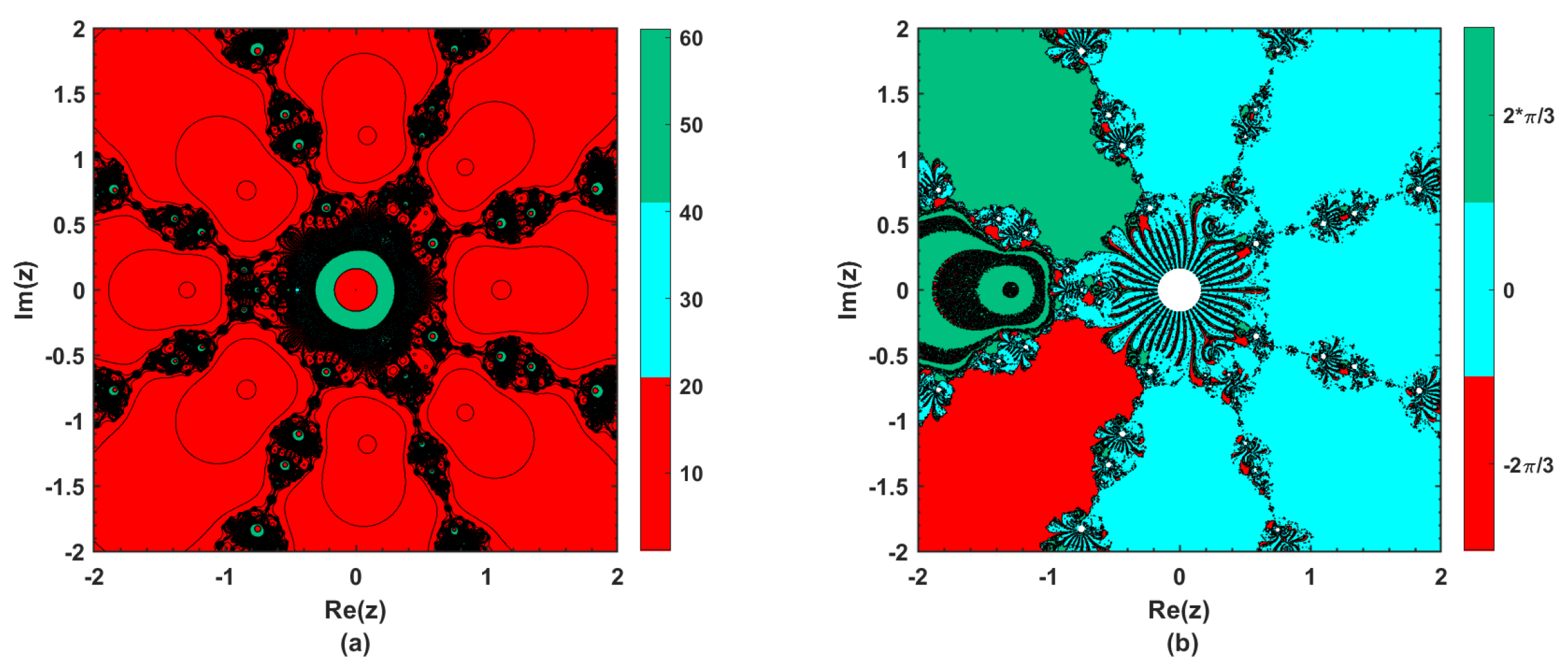
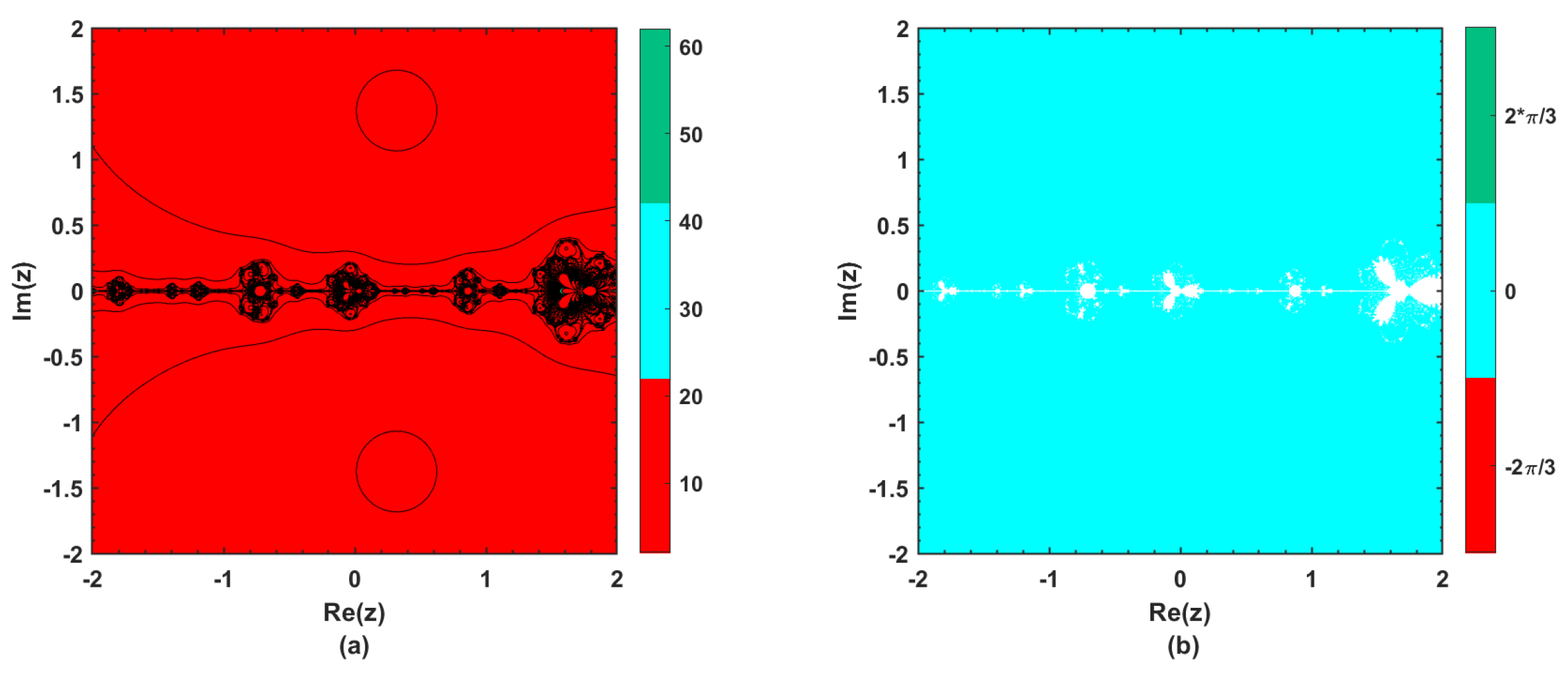
One of the dynamical concepts concerning the stability and convergence of roots for $f\left(z\right)=0$ by some iterative methods is the concept of a basin of attraction which is a region of 2D space within which iterations will be iterated into the attractor irrespective of the choice of an initial guess $z_0$. This concept is found to have several applications in scientific fields including applied mathematics, arts, design, architecture, and many more. Interesting applications of basins of attraction can be seen in the references [25,26,27,28,29] and most of the references cited therein. Nonlinear models under both scalar and vector cases have aesthetically interesting behavior that is not usually observed in the linear models. The basins of attraction will demonstrate various dynamical characteristics under the proposed iterative method PS9. Such regions, in the present study, were obtained through graphical utilities provided by some routines of MATLAB R2020a. To serve the purpose, we selected a rectangular region R on $[-2,2]\times [-2,2]$ under discretization of R into 1000 by 1000 grid points containing the solution of the complex-valued functions under consideration with considerably higher resolution. Some complex valued functions, as given below, are taken to illustrate the dynamical aspects of the behavior of PS9 via aesthetically amazing basins of attraction and their corresponding iteration coloring:

Example 1.

$$\begin{array}{cc}\hfill & P_1\left(z\right)=z^8+z^5-4,P_2\left(z\right)=z^7-1,P_3\left(z\right)=z^3-1,\hfill \\ \hfill & P_4\left(z\right)=cos\left(z\right)+cos\left(2z\right)+z,P_5\left(z\right)=exp\left(z\right)-z,P_6\left(z\right)=cosh\left(z\right)-1.\hfill \end{array}$$

(35)

The above functions were selected, randomly containing both complex polynomials and transcendental functions. Graphs were obtained with MATLAB R2020a within $R=[-2,2]\times [-2,2]$ taking $ϵ={10}^{-2}$ and $k=60$, where k refers to the maximum number of iterations chosen. It should be noted that the region R is the phase-space wherein the basins of attractions are plotted under PS9 for the complex-valued functions described in Example (1). As seen in Figure 1, Figure 2, Figure 3, Figure 4, Figure 5 and Figure 6, the highest number of iterations is required by those initial guesses that are at or near the boundaries (black lines in the figures). When the initial guess $z_0$ is taken within a small neighborhood of the exact solution, then the minimum number of iterations is needed. While running the simulations to obtain the fractal structures shown in Figure 1, Figure 2, Figure 3, Figure 4, Figure 5 and Figure 6, we computed the total average time (seconds) required by PS9 for the complex functions under consideration, as given in

Table 2. Execution time (seconds) required by PS9 for each $P_i\left(z\right),$ $i=1,2,\dots ,6$.

$P_1\left(z\right)$	$P_2\left(z\right)$	$P_3\left(z\right)$	$P_4\left(z\right)$	$P_5\left(z\right)$	$P_6\left(z\right)$
175.347	163.000	73.605	90.891	77.399	355.274

. As observed, complex functions with higher degrees (in the case of polynomials) and hyperbolic functions are computationally more expensive.

3. Numerical Experiments

In this section, we performed some numerical simulations to illustrate the performance of the proposed scheme with ninth-order convergence, i.e., PS9, as given in Equation (9). Different types of nonlinear functions of single and multi-variable character are taken into consideration. To further strengthen the results, some practical nonlinear models were also touched upon, including those used in meteorology, civil, environmental, and chemical engineering. We use the stopping criterion $\left|f\right(x_n\left)\right|\le \epsilon$, where the tolerance is chosen as $\epsilon ={10}^{-200}$ and the required precision is set to be as large as 16,000. The numerical results obtained have been tabulated, where each table contains initial guesses, the number of iterations (N), the number of function evaluations (FEs), the computational order of convergence (COC), the absolute error ($\left|\delta \right|)$), the absolute value of the underlying function at the final approximated solution ($\left|f\right(x_N\left)\right|$), and the CPU time consumed by each scheme in seconds. The COC has been estimated using the usual formula [30,31]:

$$\mathrm{COC}=\frac{log|(x_{n+1}-x_n)/(x_n-x_{n-1})|}{log|(x_n-x_{n-1})/(x_{n-1}-\left(x_{n-2}\right)|}.$$

The numerical results were performed with the Mathematica 12.1 system running under Windows 10 OS with an installed memory of 24.0 GB having a processor Intel(R) Core(TM) i7-1065G7 CPU @ 1.30 GHz speed.

The PS9 performance shows the smallest absolute error and therefore the smallest functional value along with comparable CPU times, as can be seen in

Table 3. Numerical results for problem 2 $\left(f_1\left(x\right)\right)$ with two different initial guesses.

Scheme	IG	N	FE	COC	$\left|\mathit{\delta }\right|$	$\left|\mathit{f}\right({\mathit{x}}_{\mathit{N}}\left)\right|$	CPU
NR2	−1	10	20	2	6.7844 × 10${}^{-668}$	5.0505× 10${}^{-668}$	3.48326× 10${}^{-1}$
	$-2.5$	–	–	–	–	–	cor
Halley3	−1	7	21	3	1.7886 × 10${}^{-1027}$	1.3314 × 10${}^{-1027}$	3.15791 × 10${}^{-1}$
	$-2.5$	–	–	–	–	–	cor
MHM5	−1	5	21	5	2.4273 × 10${}^{-1828}$	1.8069 × 10${}^{-1828}$	3.44944 × 10${}^{-1}$
	$-2.5$	–	–	–	–	–	cor
HD9	−1	4	20	9	8.1193 × 10${}^{-3389}$	6.0442 × 10${}^{-3389}$	4.80154 × 10${}^{-1}$
	$-2.5$	–	–	–	–	–	cor
NZ9	−1	4	28	9	2.3033 × 10${}^{-2756}$	1.7146 × 10${}^{-2756}$	4.36889 × 10${}^{-1}$
	−2.5	5	35	9	5.9162 × 10${}^{-5250}$	4.4042 × 10${}^{-5250}$	5.43948 × 10${}^{-1}$
NA9	−1	4	24	9	2.1659 × 10${}^{-2834}$	1.6124 × 10${}^{-2834}$	3.66338 × 10${}^{-1}$
	−2.5	5	30	9	3.6387 × 10${}^{-7825}$	2.7088 × 10${}^{-7825}$	4.52668 × 10${}^{-1}$
PS9	−1	4	24	9	8.0736 × 10${}^{-3066}$	6.0102 × 10${}^{-3066}$	3.70648 × 10${}^{-1}$
	−2.5	5	30	9	1.9158 × 10${}^{-12,177}$	1.4262 × 10${}^{-12,177}$	4.51775 × 10${}^{-1}$

Here, “cor” stands for “converges to other root”.

,

Table 4. Numerical results for problem 2 $\left(f_2\left(x\right)\right)$ with two different initial guesses.

Scheme	IG	N	FE	COC	$\left|\mathit{\delta }\right|$	$\left|\mathit{f}\right({\mathit{x}}_{\mathit{N}}\left)\right|$	CPU
NR2	2.5	11	22	2	5.8883 × 10${}^{-766}$	1.4618 × 10${}^{-765}$	1.87692 × 10${}^{-1}$
	3.5	11	22	2	6.3828 × 10${}^{-689}$	1.5845 × 10${}^{-688}$	1.84759 × 10${}^{-1}$
Halley3	2.5	7	21	3	8.0586 × 10${}^{-662}$	2.0005 × 10${}^{-661}$	1.98556 × 10${}^{-1}$
	3.5	7	21	3	2.4776 × 10${}^{-620}$	6.1505 × 10${}^{-620}$	1.96121 × 10${}^{-1}$
MHM5	2.5	5	20	5	2.1016 × 10${}^{-1274}$	5.2173 × 10${}^{-1274}$	1.72745 × 10${}^{-1}$
	3.5	5	20	5	6.4517 × 10${}^{-1038}$	1.6016 × 10${}^{-1037}$	1.73838 × 10${}^{-1}$
HD9	2.5	4	20	9	5.1497 × 10${}^{-2311}$	1.2784 × 10${}^{-2310}$	2.43045 × 10${}^{-1}$
	3.5	5	25	9	2.7863 × 10${}^{-14,643}$	6.9168 × 10${}^{-14,643}$	3.09526 × 10${}^{-1}$
NZ9	2.5	5	35	9	8.1082 × 10${}^{-14,876}$	2.0128 × 10${}^{-14,875}$	3.31883 × 10${}^{-1}$
	3.5	5	35	9	1.6011 × 10${}^{-13,867}$	3.9748 × 10${}^{-13,867}$	3.28469 × 10${}^{-1}$
NA9	2.5	4	24	9	1.5993 × 10${}^{-2089}$	3.9702 × 10${}^{-2089}$	2.03494 × 10${}^{-1}$
	3.5	4	24	9	9.2900 × 10${}^{-2003}$	2.3062 × 10${}^{-2002}$	2.04602 × 10${}^{-1}$
PS9	2.5	5	30	9	1.5772 × 10${}^{-15,986}$	3.9154 × 10${}^{-15,986}$	2.46626 × 10${}^{-1}$
	3.5	5	30	9	8.5836 × 10${}^{-14,976}$	2.1309 × 10${}^{-14,975}$	2.56761 × 10${}^{-1}$

,

Table 5. Numerical results for problem 2 $\left(f_3\left(x\right)\right)$ with two different initial guesses.

Scheme	IG	N	FE	COC	$\left|\mathit{\delta }\right|$	$\left|\mathit{f}\right({\mathit{x}}_{\mathit{N}}\left)\right|$	CPU
NR2	3	17	34	2	1.3237 × 10${}^{-507}$	1.0485 × 10${}^{-503}$	2.93632 × 10${}^{-2}$
	10	12	24	2	1.0211 × 10${}^{-723}$	8.0883 × 10${}^{-720}$	1.49337 × 10${}^{-2}$
Halley3	3	8	24	3	4.5761 × 10${}^{-734}$	3.6249 × 10${}^{-730}$	3.1627 × 10${}^{-2}$
	10	8	24	3	1.0770 × 10${}^{-1618}$	8.5316 × 10${}^{-1615}$	1.58703 × 10${}^{-2}$
MHM5	3	7	28	5	1.4757 × 10${}^{-1057}$	1.1690 × 10${}^{-1053}$	3.45364 × 10${}^{-2}$
	10	6	24	5	4.5028 × 10${}^{-4545}$	3.5669 × 10${}^{-4541}$	1.88998 × 10${}^{-2}$
HD9	3	6	30	9	3.3382 × 10${}^{-2585}$	2.6444 × 10${}^{-2581}$	5.35406 × 10${}^{-2}$
	10	5	25	9	1.4417 × 10${}^{-9726}$	1.1420 × 10${}^{-9722}$	2.13777 × 10${}^{-2}$
NZ9	3	12	84	9	2.0186 × 10${}^{-4985}$	1.5991 × 10${}^{-4981}$	6.30927 × 10${}^{-2}$
	10	5	35	9	4.7604 × 10${}^{-9218}$	3.7710 × 10${}^{-9214}$	2.2781 × 10${}^{-2}$
NA9	3	18	108	9	1.4323 × 10${}^{-5353}$	1.1346 × 10${}^{-5349}$	7.6371 × 10${}^{-2}$
	10	6	36	9	1.2447 × 10${}^{-3038}$	9.8598 × 10${}^{-3035}$	2.16169 × 10${}^{-2}$
PS9	3	9	54	9	1.1880 × 10${}^{-12,908}$	9.4106 × 10${}^{-12,905}$	4.76255 × 10${}^{-2}$
	10	5	30	9	2.6095 × 10${}^{-11,353}$	2.0671 × 10${}^{-11,349}$	1.89325 × 10${}^{-2}$

,

Table 6. Numerical results for problem 2 $\left(f_4\left(x\right)\right)$ with two different initial guesses.

Scheme	IG	N	FE	COC	$\left|\mathit{\delta }\right|$	$\left|\mathit{f}\right({\mathit{x}}_{\mathit{N}}\left)\right|$	CPU
NR2	−5	–	–	–	–	–	div
	−1/3	9	18	2	2.1180 × 10${}^{-466}$	4.9528 × 10${}^{-466}$	2.11767 × 10${}^{-1}$
Halley3	−5	27	81	3	2.3382 × 10${}^{-1038}$	5.4678 × 10${}^{-1038}$	8.57785 × 10${}^{-1}$
	−1/3	7	21	3	7.8648 × 10${}^{-1170}$	1.8392 × 10${}^{-1169}$	2.40809 × 10${}^{-1}$
MHM5	−5	9	36	5	1.1386 × 10${}^{-3306}$	2.6626 × 10${}^{-3306}$	3.8909 × 10${}^{-1}$
	−1/3	5	20	5	1.6473 × 10${}^{-1913}$	3.8522 × 10${}^{-1913}$	2.24586 × 10${}^{-1}$
HD9	−5	11	55	9	1.8961 × 10${}^{-6163}$	4.4340 × 10${}^{-6163}$	8.1018 × 10${}^{-1}$
	−1/3	4	20	9	7.7641 × 10${}^{-3675}$	1.8156 × 10${}^{-3674}$	3.12411 × 10${}^{-1}$
NZ9	−5	–	–	–	–	–	div
	−1/3	4	28	9	7.3808 × 10${}^{-2379}$	1.7260 × 10${}^{-2378}$	3.19858 × 10${}^{-1}$
NA9	−5	–	–	–	–	–	div
	−1/3	4	24	9	2.1249 × 10${}^{-2426}$	4.9690 × 10${}^{-2426}$	2.64398 × 10${}^{-1}$
PS9	−5	6	36	9	7.8317 × 10${}^{-15,259}$	1.8314 × 10${}^{-15,258}$	3.7976 × 10${}^{-1}$
	−1/3	4	24	9	2.7500 × 10${}^{-4036}$	6.4307 × 10${}^{-4036}$	2.72867 × 10${}^{-1}$

Here, “div” stands for “divergence”.

and

Table 7. Numerical results for problem 2 $\left(f_5\left(x\right)\right)$ with two different initial guesses.

Scheme	IG	N	FE	COC	$\mathit{\delta }$	$\left|\mathit{f}\right({\mathit{x}}_{\mathit{N}}\left)\right|$	CPU
NR2	1	10	20	2	3.5191 × 10${}^{-674}$	9.7264 × 10${}^{-674}$	1.47033 × 10${}^{-1}$
	8 × 10${}^{-1}$	–	–	–	–	–	div
Halley3	1	8	24	3	3.5230 × 10${}^{-1414}$	9.7372 × 10${}^{-1414}$	1.92348 × 10${}^{-1}$
	8 × 10${}^{-1}$	9	27	3	7.2446 × 10${}^{-1345}$	2.0023 × 10${}^{-1344}$	2.23313 × 10${}^{-1}$
MHM5	1	5	20	5	9.4742 × 10${}^{-1903}$	2.6186 × 10${}^{-1902}$	1.50974 × 10${}^{-1}$
	8 × 10${}^{-1}$	–	–	–	–	–	div
HD9	1	4	20	8.9999	5.9828 × 10${}^{-2649}$	1.6536 × 10${}^{-2648}$	2.10601 × 10${}^{-1}$
	8 × 10${}^{-1}$	6	30	8.9999	2.3478 × 10${}^{-2593}$	6.4892 × 10${}^{-2593}$	3.11126 × 10${}^{-1}$
NZ9	1	5	35	9	1.0297 × 10${}^{-4910}$	2.8460 × 10${}^{-4910}$	3.10084 × 10${}^{-1}$
	8 × 10${}^{-1}$	–	–	–	–	–	div
NA9	1	5	30	9	2.0815 × 10${}^{-8678}$	5.7532 × 10${}^{-8678}$	2.14216 × 10${}^{-1}$
	8 × 10${}^{-1}$	–	–	–	–	–	div
PS9	1	5	30	9	4.8523 × 10${}^{-12,769}$	1.3411 × 10${}^{-12,768}$	2.14661 × 10${}^{-1}$
	8 × 10${}^{-1}$	5	30	9	5.1698 × 10${}^{-11,170}$	1.4289 × 10${}^{-11,169}$	2.20604 × 10${}^{-1}$

for the five test functions listed in problem 2. Under different initial guesses taken near and far from the approximate roots, it can be seen from these tables that the proposed strategy takes reasonable and sometimes smaller iterations to meet the stopping criteria. The COC turns out to be 9, confirming the theoretical ninth-order of convergence derived in Section 2.2.1. The functional absolute values at the last approximation considered and the corresponding absolute errors are smaller with PS9 compared to other schemes, while consuming a reasonable amount of CPU time. Moreover, schemes given as NR2, NZ9 and NA9 in [5,23,24], respectively, could not produce results for the test functions $f_4\left(x\right)$ under the initial guess $x_0=-5$, and $f_5\left(x\right)$ under the initial guess $x_0=0.8$ including the scheme MHM5.

Example 2.

$$\begin{array}{cc}\hfill & f_1\left(x\right)=log(x^2+1)+exp\left(x\right)sin\left(x\right),\hfill \\ \hfill & x^{\star }\approx -0.6032319715572151673731685726070837720365.\hfill \\ \hfill & f_2\left(x\right)={sin}^2\left(x\right)-x^2+1,\hfill \\ \hfill & x^{\star }\approx 1.4044916482153412260350868177868680771766.\hfill \\ \hfill & f_3\left(x\right)=x^5+x-10000,\hfill \\ \hfill & x^{\star }\approx 6.3087771299726890947675717717830591133776.\hfill \\ \hfill & f_4\left(x\right)=sin\left(x\right)+cos\left(x\right)+x,\hfill \\ \hfill & x^{\star }\approx -0.4566247045676308244376974571284573758982.\hfill \\ \hfill & f_5\left(x\right)=10xexp(-x^2)-1,\hfill \\ \hfill & x^{\star }\approx 1.6796306104284499406749203388379703978290.\hfill \end{array}$$

(36)

Example 3.

Open-channel flow.

In civil and environmental engineering, it remains a challenge to relate the water flow with factors affecting the flow within open channels including canals, drainage ditches, gutters, and sewers. Such a flow rate is defined to be the volume of flow passing a particular point through an area during a selected period. However, another problematic situation occurs when the channel under consideration becomes sloppy. The following Manning’s equation comes into play for the water flow in an open channel that is flowing under uniform flow conditions:

$$Q={\displaystyle \frac{\sqrt{m}}{n}}A{R}^{2/3},$$

(37)

where m is the slope of the channel, A is the cross-sectional area of the channel, R is the hydraulic radius of the channel and n is the Manning’s roughness coefficient. For a rectangular channel having the width W and the depth of water in the channel h, it is known that $A=Wh,$ and:

$$R={\displaystyle \frac{Wh}{W+2h}}.$$

(38)

With these values, (37) becomes:

$$Q={\displaystyle \frac{\sqrt{m}}{n}}Wh{\left[{\displaystyle \frac{Wh}{W+2h}}\right]}^{2/3}.$$

(39)

As per the requirement wherein one needs to determine the depth of water h in the channel for a given quantity of water, the above equation can be rewritten as follows:

$$f\left(h\right)={\displaystyle \frac{\sqrt{m}}{n}}Wh{\left[{\displaystyle \frac{Wh}{W+2h}}\right]}^{2/3}-Q.$$

(40)

The depth of water h in the channel has been estimated while assuming the rest of the parameters as $Q=14.15$ m${}^3$/s, $W=4.572$ m, $n=0.017$ and $m=0.0015$. The initial guess is taken to be $h_0=8.5$ m. The numerical results under different schemes are shown in

Table 8. Numerical results for the problem 3 with the initial guess $h_0=8.5$ m.

Scheme	N	FE	COC	$\left|\mathit{\delta }\right|$	$\left|\mathit{f}\right({\mathit{x}}_{\mathit{N}}\left)\right|$	CPU
NR2	10	20	2	2.9995 × 10${}^{-753}$	4.0739 × 10${}^{-752}$	5.56574 × 10${}^{-2}$
Halley3	7	21	3	4.7746 × 10${}^{-947}$	6.4848 × 10${}^{-946}$	8.73257 × 10${}^{-2}$
MHM5	5	20	5	4.1591 × 10${}^{-1797}$	5.6489 × 10${}^{-1796}$	5.60582 × 10${}^{-2}$
HD9	4	20	9	7.4120 × 10${}^{-3264}$	1.0067 × 10${}^{-3262}$	8.84709 × 10${}^{-2}$
NZ9	4	28	9	3.8534 × 10${}^{-2588}$	5.2337 × 10${}^{-2587}$	1.33463 × 10${}^{-1}$
NA9	4	24	9	1.4631 × 10${}^{-2431}$	1.9872 × 10${}^{-2430}$	7.27594 × 10${}^{-2}$
PS9	4	24	9	1.1984 × 10${}^{-3119}$	1.6277 × 10${}^{-3118}$	8.00343 × 10${}^{-2}$

. It can be observed from this table that the functional value and the absolute error are smallest with HD9, whereas PS9 competes well enough and consumes less time while maintaining ninth-order convergence, as given by COC in the fourth column of Table 8.

Example 4.

Planck’s radiation law.

Consider the following Planck’s radiation law problem:

$$\varphi \left(\lambda \right)={\displaystyle \frac{8\pi ch{\lambda }^{-5}}{exp(ch/\lambda kT)-1}},$$

(41)

which calculates the energy density within an isothermal blackbody. Here, $\lambda$ stands for the wavelength of the radiation, T is the absolute temperature of the blackbody, k is Boltzmann’s constant, h is the Planck’s constant, and c shows the speed of light. Here, we compute the wavelength $\lambda$ which corresponds to the maximum energy density $\varphi \left(\lambda \right)$. Using (41), we obtain:

$${\varphi }^{\prime }\left(\lambda \right)={\displaystyle \frac{8\pi ch}{{\lambda }^{7}kT{(exp(ch/\lambda kT)-1)}^2}}\left[5\lambda kT+(-5\lambda kT+ch)exp(ch/\lambda kT)\right],$$

(42)

or:

$${\varphi }^{\prime }\left(\lambda \right)=\left[{\displaystyle \frac{8\pi ch{\lambda }^{-6}}{exp(ch/\lambda kT)-1}}\right]\left[{\displaystyle \frac{(ch/\lambda kT)exp(ch/\lambda kT)}{exp(ch/\lambda kT)-1}}-5\right]=LM.$$

(43)

It is easy to see that a maximum for $\varphi$ occurs when M = 0, that is, when:

$${\displaystyle \frac{(ch/\lambda kT)exp(ch/\lambda kT)}{exp(ch/\lambda kT)-1}}=5.$$

(44)

Substituting $x=ch/\lambda kT$, the above equation can be rewritten as

$$exp(-x)-1+{\displaystyle \frac{x}{5}}=0.$$

(45)

The numerical results from the application problem 4 regarding Planck’s radiations are listed in

Table 9. Numerical results for the problem 4 with initial guess $x_0=1.5$ m.

Scheme	N	FE	COC	$\left|\mathit{\delta }\right|$	$\left|\mathit{f}\right({\mathit{x}}_{\mathit{N}}\left)\right|$	CPU
NR2	–	–	–	–	–	cor
Halley3	–	–	–	–	–	cor
MHM5	–	–	–	–	–	cor
HD9	–	–	–	–	–	cor
NZ9	4	28	8.9980	8.6591 × 10${}^{-1833}$	1.6714 × 10${}^{-1833}$	1.83824 × 10${}^{-1}$
NA9	4	24	8.9980	3.7106 × 10${}^{-1820}$	7.1623 × 10${}^{-1821}$	1.58117 × 10${}^{-1}$
PS9	5	30	9	3.9539 × 10${}^{-6413}$	7.6320 × 10${}^{-6414}$	1.48649 × 10${}^{-1}$

in which it is observed that the functional value and the corresponding absolute error are smaller under PS9 with a reasonable amount of CPU time while taking only five iterations to meet the stopping criterion. It is worth noting that the schemes NR2, Halley3, MHM5, and HD9 converge to a solution other than the required one.

Example 5.

Volume from van der Waals equation.

A well-known model from chemistry used for determining the difference between ideal and real gases is known as the van der Waals nonlinear equation which is given as follows:

$$\left[P+{\displaystyle \frac{n^{2}k}{V^2}}\right](V-nh)=nRT,$$

(46)

where k and h are the positive real parameters also known as the van der Waals constants which depend on the type of gas under consideration. Moreover, constants $P,V,T$ are the pressure, volume, and temperature of the gas. $R\approx 0.0820578$ is the gas constant and n represents the number of moles. The equation given above is simplified as follows:

$$f\left(V\right)=P{V}^3-V^2(RT+hP)n+n^{2}kV-hk{n}^3.$$

(47)

The following third degree polynomial can be obtained under $k=18,$ $h=0.1154,$ $n=1.4,P=40$ atm, and $T=500{}^{\circ }$C:

$$40V^3-95.26535116V^2+35.28V-5.6998368=0.$$

(48)

The approximate solution of (48) correct to 40 dp is as follows:

2.1544346900318837217592935665193504952593.

We solved the Equation (48) with the schemes under consideration taking $V_0=0.0$, resulting in the data shown in

Table 10. Numerical results for the problem 5 with the initial guess $V_0=0.0$ m.

Scheme	N	FE	COC	$\left|\mathit{\delta }\right|$	$\left|\mathit{f}\right({\mathit{x}}_{\mathit{N}}\left)\right|$	CPU
NR2	43	86	2	3.6193 × 10${}^{-437}$	4.5554 × 10${}^{-435}$	6.41579 × 10${}^{-2}$
Halley3	67	201	3	9.3314 × 10${}^{-649}$	1.1745 × 10${}^{-646}$	8.29023 × 10${}^{-2}$
MHM5	66	264	5	1.1626 × 10${}^{-2639}$	1.4634 × 10${}^{-2637}$	1.32827 × 10${}^{-1}$
HD9	33	165	9	1.3850 × 10${}^{-5655}$	1.7433 × 10${}^{-5653}$	1.15104 × 10${}^{-1}$
NZ9	12	84	9	1.2468 × 10${}^{-4992}$	1.5693 × 10${}^{-4990}$	4.8313 × 10${}^{-2}$
NA9	14	84	9	2.1302 × 10${}^{-12,469}$	2.6812 × 10${}^{-12,467}$	5.24887 × 10${}^{-2}$
PS9	9	54	9	9.5118 × 10${}^{-11,767}$	1.1972 × 10${}^{-11,764}$	2.63721 × 10${}^{-2}$

. It can be observed that PS9 produces the smallest absolute error with the least CPU time, followed by the ninth-order scheme NA9. Each scheme, for this particular problem, needs many more iterations than PS9. This applied problem shows the highest performance of PS9 in terms of number of iterations, number of function evaluations, absolute error, absolute functional value and CPU time.

The schemes NR2 and PS9 have been used for solving two nonlinear three-dimensional systems given by problems 6 and 7. Here, we chose only NR2 and PS9 because the simulations obtained under other schemes behave dynamically in the same way as that shown in the univariate cases discussed above. For the steady-state of the Lorenz Equations (49) and the system (51),

Table 11. Numerical results for problem 6 with different initial guesses.

Scheme	IG	N	$\left|\mathit{f}\right({\mathit{x}}_{\mathit{N}}\left)\right|$	$\mathit{\delta }$	CPU
NR2	${[2,2,2]}^T$	10	${[0,7\times {10}^{-633},1\times {10}^{-632}]}^T$	$7\times {10}^{-632}$	$1.5047\times {10}^{-1}$
PS9	–	4	${[0,6\times {10}^{-3692},1\times {10}^{-3691}]}^T$	$8\times {10}^{-3692}$	$2.1441\times {10}^{-1}$
NR2	${[1,1,1]}^T$	10	${[0,0,3\times {10}^{-585}]}^T$	$1\times {10}^{-585}$	$1.2649\times {10}^{-1}$
PS9	–	4	${[0,0,5\times {10}^{-3496}]}^T$	$2\times {10}^{-3496}$	$2.1011\times {10}^{-1}$
NR2	${[0.7,3.2,2.7]}^T$	20	${[0,1\times {10}^{-452},2\times {10}^{-452}]}^T$	$2\times {10}^{-452}$	$2.6031\times {10}^{-1}$
PS9	–	5	${[0,1\times {10}^{-7030},2\times {10}^{-7030}]}^T$	$2\times {10}^{-7030}$	$2.9860\times {10}^{-1}$

and

Table 12. Numerical results for problem 7 with different initial guesses.

Scheme	IG	N	$\left|\mathit{f}\right({\mathit{x}}_{\mathit{N}}\left)\right|$	$\mathit{\delta }$	CPU
NR2	$[1,1,1]$	10	$[2\times {10}^{-648},6\times {10}^{-645},5\times {10}^{-648}]$	$2\times {10}^{-646}$	$1.00\times {10}^0$
PS9	–	5	$[3\times {10}^{-3994},1\times {10}^{-3992},3\times {10}^{-3994}]$	$1\times {10}^{-3992}$	$1.18\times {10}^0$
NR2	${[3,2,-2]}^T$	10	$[1\times {10}^{-749},6\times {10}^{-747},8\times {10}^{-750}]$	$4\times {10}^{-748}$	$1.23\times {10}^0$
PS9	–	5	$[1\times {10}^{-2076},6\times {10}^{-2074},9\times {10}^{-2077}]$	$4\times {10}^{-2075}$	$1.15\times {10}^0$
NR2	${[7,1,-4]}^T$	10	$[9\times {10}^{-495},5\times {10}^{-492},8\times {10}^{-495}]$	$2\times {10}^{-1}$	$8.50\times {10}^{-1}$
PS9	–	6	$[2\times {10}^{-6869},1\times {10}^{-6866},2\times {10}^{-6869}]$	$7\times {10}^{-6868}$	$1.16\times {10}^0$

show that, at little high computational cost, PS9 yields the smallest error norm ${\delta }_{n+1}=\left|\right|{\mathit{x}}_{n+1}-{\mathit{x}}_n{\left|\right|}_{\infty }$ and the smallest absolute functional values under different initial conditions. Additionally, PS9 takes very few iterations to meet the stopping criterion. The numerical results of these two systems are in favor of PS9, showing that PS9 is applicable for both univariate (single nonlinear equation) and multivariate (system of nonlinear equations) cases, while maintaining its ninth-order convergence.

Example 6.

Lorenz system in steady-state [32] (p. 816)

$$\begin{array}{cc}\hfill & x_1-x_2=0,\hfill \\ \hfill & 2x_1-x_1{x}_3-x_2=0,\hfill \\ \hfill & x_1{x}_2-3x_3=0.\hfill \end{array}$$

(49)

The approximate solution for the system (49) correct to 50 dp is given by

$$\mathit{x}\approx \left[\begin{array}{c}1.7320508075688772935274463415058723669428052538104\\ 1.7320508075688772935274463415058723669428052538104\\ 1\end{array}\right].$$

(50)

Example 7.

Another nonlinear system of three equations, taken from [33], is:

$$\begin{array}{cc}\hfill & 3x_1-cos\left(x_2{x}_3\right)-1/2=0,\hfill \\ \hfill & x_1^2-81{(x_2+0.1)}^2+sin\left(x_3\right)+1.06=0,\hfill \\ \hfill & exp(-x_1{x}_2)+20x_3+(10\pi /3-1)=0,\hfill \end{array}$$

(51)

where its approximate solution up to 50 dp is:

$$\mathit{x}\approx \left[\begin{array}{c}0.49814468458949119126228211413809456132099782481239\\ 0\\ -0.52882597757338745562224205210357569604547206124467\end{array}\right].$$

(52)

The numerical results for the system (51) are shown in Table 12 showing the good performance of the proposed method.

4. Concluding Remarks

A new ninth-order convergent scheme, with six function evaluations per iteration, to solve nonlinear models in both univariate and multivariate cases is proposed by blending a third-order modified Newton’s and the third-order Halley’s schemes. The theoretical order of convergence with the asymptotic error term was obtained via Taylor’s expansion and the efficiency index was calculated to be approximately 1.4422. The proposed scheme was found to be accurate and reliable enough in terms of iteration counts, number of function evaluations, absolute errors, and CPU time. This was further confirmed when the schemes under consideration were used to solve several applied models in different fields. Two-dimensional phase diagrams, using the proposed scheme, were obtained to show basins of attraction for the stability of PS9.

The presented scheme (9), which comes in the category of the schemes without memory, requires the evaluation of three inverse operators per iteration. In addition, such schemes also require many multiplication and division operations while computing derivatives and inverse operators. All such evaluations will increase, to some extent, the amount of computational work of the scheme. Thus, future work would include the modification of PS9 as a numerical scheme with memory, keeping in mind the time efficiency and the computational complexity. Moreover, first- and second-order derivatives involved in PS9 can be replaced using appropriate finite-difference approximations to avoid complexity with the analytical expressions. Such analyses will be carried out in our future research studies.

References

- Kaplan, E. Understanding GPS: Principles and Applications; Artech House: Boston, MA, USA, 1996. [Google Scholar]
- Rouzbar, R.; Eyi, S. Reacting flow analysis of a cavity-based scramjet combustor using a Jacobian-free Newton–Krylov method. Aeronaut. J. 2018, 122, 1884–1915. [Google Scholar] [CrossRef]
- Nourgaliev, R.; Greene, P.; Weston, B.; Barney, R.; Anderson, A.; Khairallah, S.; Delplanque, J.P. High-order fully implicit solver for all-speed fluid dynamics. Shock Waves 2019, 29, 651–689. [Google Scholar] [CrossRef]
- Zhang, H.; Guo, J.; Lu, J.; Niu, J.; Li, F.; Xu, Y. The comparison between nonlinear and linear preconditioning JFNK method for transient neutronics/thermal-hydraulics coupling problem. Ann. Nucl. Energy 2019, 132, 357–368. [Google Scholar] [CrossRef]
- Traub, J.F. Iterative Methods for the Solution of Equations; American Mathematical Society: Providence, RI, USA, 1982; Volume 312. [Google Scholar]
- Rafiullah, M. A fifth-order iterative method for solving nonlinear equations. Numer. Anal. Appl. 2011, 4, 239–243. [Google Scholar] [CrossRef]
- Ganji, D.D. The application of He’s homotopy perturbation method to nonlinear equations arising in heat transfer. Phys. Lett. A 2006, 355, 337–341. [Google Scholar] [CrossRef]
- Abbasbandy, S. Improving Newton–Raphson method for nonlinear equations by modified Adomian decomposition method. Appl. Math. Comput. 2003, 145, 887–893. [Google Scholar] [CrossRef]
- He, J.H.; Wu, X.H. Variational iteration method: New development and applications. Comput. Math. Appl. 2007, 54, 881–894. [Google Scholar] [CrossRef] [Green Version]
- Tari, H.; Ganji, D.D.; Babazadeh, H. The application of He’s variational iteration method to nonlinear equations arising in heat transfer. Phys. Lett. A 2007, 363, 213–217. [Google Scholar] [CrossRef]
- Noor, M.A.; Waseem, M. Some iterative methods for solving a system of nonlinear equations. Comput. Math. Appl. 2009, 57, 101–106. [Google Scholar] [CrossRef] [Green Version]
- Zafar, F.; Mir, N.A. A generalized family of quadrature based iterative methods. Gen. Math. 2010, 18, 43–51. [Google Scholar]
- Cordero, A.; Hueso, J.L.; Martínez, E.; Torregrosa, J.R. A modified Newton–Jarratt’s composition. Numer. Algorithms 2010, 55, 87–99. [Google Scholar] [CrossRef]
- Noor, M.A.; Noor, K.I. Three-step iterative methods for nonlinear equations. Appl. Math. Comput. 2006, 183, 322–327. [Google Scholar]
- Noor, M.A.; Noor, K.I.; Al-Said, E.; Waseem, M. Some new iterative methods for nonlinear equations. Math. Probl. Eng. 2010, 2010, 198943. [Google Scholar] [CrossRef]
- Shah, F.A.; Noor, M.A.; Waseem, M. Some second-derivative-free sixth-order convergent iterative methods for non-linear equations. Maejo Int. J. Sci. Technol. 2016, 10, 79. [Google Scholar]
- Abro, H.A.; Shaikh, M.M. A new time-efficient and convergent nonlinear solver. Appl. Math. Comput. 2019, 355, 516–536. [Google Scholar] [CrossRef]
- Darvishi, M.T.; Barati, A. A third-order Newton-type method to solve systems of nonlinear equations. Appl. Math. Comput. 2007, 187, 630–635. [Google Scholar] [CrossRef]
- Torregrosa, J.R.; Argyros, I.K.; Chun, C.; Cordero, A.; Soleymani, F. Iterative methods for nonlinear equations or systems and their applications 2014. J. Appl. Math. 2014, 2014, 293263. [Google Scholar] [CrossRef] [Green Version]
- Chen, D.; Argyros, I.K.; Qian, Q.S. A note on the Halley method in Banach spaces. Appl. Math. Comput. 1983, 58, 215–224. [Google Scholar] [CrossRef]
- Noor, M.A.; Khan, W.A.; Hussain, A. A new modified Halley method without second derivatives for nonlinear equation. Appl. Math. Comput. 2007, 189, 1268–1273. [Google Scholar] [CrossRef]
- Ding, H.F.; Zhang, Y.X.; Wang, S.F.; Yang, X.Y. A note on some quadrature based three-step iterative methods for non-linear equations. Appl. Math. Comput. 2009, 215, 53–57. [Google Scholar] [CrossRef]
- Nazeer, W.; Nizami, A.R.; Tanveer, M.; Sarfraz, I. A ninth-order iterative method for nonlinear equations along with polynomiography. J. Prime Res. Math. 2017, 13, 41–55. [Google Scholar]
- Naseem, A.; Rehman, M.A.; Abdeljawad, T. Higher-Order Root-Finding Algorithms and Their Basins of Attraction. J. Math. 2020, 2020, 5070363. [Google Scholar] [CrossRef]
- Scott, M.; Neta, B.; Chun, C. Basin attractors for various methods. Appl. Math. Comput. 2011, 218, 2584–2599. [Google Scholar] [CrossRef]
- Stewart, B.D. Attractor Basins of Various Root-Finding Methods; Naval Postgraduate School: Monterey, CA, USA, 2001. [Google Scholar]
- Halley, E. A new, exact, and easy method of finding the roots of any equations generally, and that without any previous reduction. Philos. Trans. Roy. Soc. Lond. 1694, 18, 136–145. [Google Scholar] [CrossRef] [Green Version]
- Chen, H.; Zheng, X. Improved Newton Iterative Algorithm for Fractal Art Graphic Design. Complexity 2020, 2020, 6623049. [Google Scholar] [CrossRef]
- Susanto, H.; Karjanto, N. Newton’s method’s basins of attraction revisited. Appl. Math. Comput. 2009, 215, 1084–1090. [Google Scholar] [CrossRef] [Green Version]
- Weerakoon, S.; Fernando, T.G.I. A variant of Newton’s method with accelerated third-order convergence. Appl. Math. Lett. 2000, 13, 87–93. [Google Scholar] [CrossRef]
- Grau-Sánchez, M.; Noguera, M.; Gutiérrez, J.M. On some computational orders of convergence. Appl. Math. Lett. 2010, 23, 472–478. [Google Scholar] [CrossRef] [Green Version]
- Chapra, S.C.; Canale, R.P. Numerical Methods for Engineers; McGraw-Hill Higher Education: Boston, MA, USA, 2010. [Google Scholar]
- Burden, R.L.; Faires, J.D. Numerical Analysis; Brooks/Cole, Cengage Learning: Boston, MA, USA, 2011. [Google Scholar]
Figure 1.
The polynomiographs obtained by the proposed method PS9 for .
Figure 2.
Figure 3.
Figure 4.
Figure 5.
Figure 6.