1. Introduction
Throughout this paper, we let
H be a real Hilbert space with the norm
and the inner product
, respectively,
C be a nonempty closed convex subset of
H and
be a mapping. We recall the variational inequality problem (VIP) is to find a point
such that
We denote the solution set of VIP (
1) by
.
The variational inequality problem is one of the most important problems in nonlinear analysis. Now, this problem has been studied by many scholars.
In 2000, Tseng [
1] introduced the following method:
where
A is monotone and
L-Lipschitzian (see in
Section 2, Definition 1),
,
. This algorithm has a weak convergence result.
In 2011, Censor et al. [
2] proposed the subgradient extragradient method for solving VIP (
1), as follows:
The conditions of A and are the same as those in Tseng’s method. Then the sequence converges weakly to some point under some conditions.
In recent years, some scholars have paid attention to the following hierarchical variational inequality problems (HVIP):
where
is a strongly monotone and Lipschitzian mapping.
In 2020, Hieu et al. [
3,
4] proposed regularized subgradient extragradient method (Algorithm 1 RSEGM) and regularized Tseng’s extragradient method (Algorithm 2 RTEGM) for solving HVIP (
4). Both of these two methods have strong convergence results.
On the other hand, in order to accelerate the convergence, the inertial methods have been studied extensively by many scholars [
5,
6,
7,
8,
9,
10,
11,
12]. One of the important results is the inertial Mann algorithm which is introduced by Maingé [
5] in 2007:
Under some conditions, the sequence converges weakly to a fixed point of T.
In 2019, Dong et al. [
7] proposed the multi-step inertial Krasnosel’skiĭ-Mann algorithm for finding a fixed point of a nonexpansive mapping, as follows:
This algorithm has a weak convergence result under certain conditions.
In this paper, motivated by the results of [
3,
4,
7], we construct a multi-step inertial regularized subgradient extragradient method and a multi-step inertial regularized Tseng’s extragradient method for solving HVIP (
4) in a Hilbert space when
F is a generalized Lipschitzian and hemicontinuous mapping (see in
Section 2, Definitions 2 and 3). Then, we present two strong convergence theorems and give some numerical experiments to show the effectiveness and feasibility of our new iterative methods.
| Algorithm 1 Regularized subgradient extragradient method (RSEGM) |
|
| Algorithm 2 Regularized Tseng’s extragradient method (RTEGM) |
|
2. Preliminaries
In this section, we present some necessary definitions and lemmas which are needed for our main results.
Definition 1 ([
13]).
Let be a mapping.- (i)
A is ζ-strongly monotone () if - (ii)
- (iii)
A is L-Lipschitzian () if
Let be a sequence. We use and to indicate that converges strongly and weakly to z, respectively.
Definition 2 ([
14]).
Let be a mapping. A is said to be hemicontinuous if , , implies as . It is obvious that a continuous mapping must be hemicontinuous, but the converse is not true.
Lemma 1 ([
14]).
If be a hemicontinuous and strongly monotone mapping in VIP (1), then VIP (1) exists a unique solution. Lemma 2 ([
15]).
If be a monotone and hemicontinuous mapping. Then if and only if , . Definition 3 ([
14]).
Let be a mapping. A is said to be L-generalized Lipschitzian () if Remark 1. We can easily see that a Lipschitzian mapping must be a generalized Lipschitzian mapping, but the converse is not true. A generalized Lipschitzian mapping may even not be hemicontinuous. For example, consider the sign function , defined by Then f is generalized Lipschitzian but not hemicontinuous [14]. A continuous generalized Lipschitzian mapping may not be Lipschitzian. For example, let be defined by We can see that g is continuous and generalized Lipschitzian but not Lipschitzian. In the past, many scholars studied Lipschitzian mappings, but in this paper, we pay attention to generalized Lipschitzian. Therefore, the research in this paper is meaningful.
Recall the metric projection operator
from
H onto
C, defined as follows:
Lemma 3 ([
16,
17]).
Given and , we have- (i)
- (ii)
is firmly nonexpansive, i.e., - (iii)
.
The following lemma is important to prove the strong convergence.
Lemma 4 ([
18,
19]).
Let be a sequence of nonnegative real numbers satisfyingwhere , and satisfy the following conditions:- (i)
with ;
- (ii)
;
- (iii)
with .
Then .
Now, we focus on HVIP (
4) when
A and
F satisfy the following conditions:
(CD1) A is monotone on C and L-Lipschitzian on H.
(CD2) F is -strongly monotone, K-generalized Lipschitzian and hemicontinuous on H.
(CD3) is nonempty.
From Lemma 1, we know that HVIP (
4) exists the unique solution if the conditions (CD1)–(CD3) are satisfied. We denote this solution by
. Consider the following variational inequality problem:
where
,
A and
F satisfy conditions (CD1)–(CD3). It is obvious that
is strongly monotone and hemicontinuous, so VIP (
7) has the unique solution according to Lemma 1. We denote this solution by
.
We have the following lemmas.
Lemma 5. .
Proof. For each
, since
is the solution of VIP (2.1), we have
and
Adding the inequalities above, we obtain
Since
A is monotone on
C, we get
Adding (
8) and (
9), we obtain
which means
From the
-strongly monotonicity of
F, we get
Adding (
10) and (
11), we obtain
Particularly, this is also true for . □
Lemma 6. For all , , where M is a positive constant. More precisely, .
Proof. Since
and
, we have
and
Adding the two inequalities above, we obtain
which, by the monotonicity of
A, implies that
From the
-strong monotonicity of
F, we obtain
Substituting the last relation into (
15), we have
which means
Since
F is generalized Lipschitzian, by Lemma 5, we get
Substituting (
17) into (
16), we obtain
where
. □
Lemma 7. .
Proof. From Lemma 5, we know that
is bounded. So there exists a sequence
such that
and
as
by the reflexivity of
H. Since
is the solution of VIP (
7), we have
which, by the monotonicity of
A, implies that
Replacing
with
in the last relation, we get
Since
is bounded and
F is generalized Lipschitzian,
is also bounded. Taking limit in (
19), we obtain
It follows from Lemma 2 that
. From (
12), we deduce
Taking limit in (
21), we obtain
It means that
is a solution of HVIP (
6). Since HVIP (
6) has the unique solution
, we conclude
. Thus,
as
. Replacing
u with
in (
12), we get
It follows from the fact that . □
3. Multi-Step Inertial RSEGM
In this section, we propose a new multi-step inertial method for solving HVIP (
4) based on Algorithm 1 (RSEGM). Under certain conditions, it has a strong convergence result.
We need the following lemma to analyze the convergence of generated by Algorithm 3.
Lemma 8 ([
20]).
The sequence generated by Algorithm 3 is non-increasing andMore precisely, we have .
Theorem 1. Under the conditions (CD1)–(CD3), the sequence generated by Algorithm 3 converges strongly to , where is the unique solution of HVIP (4). | Algorithm 3 Multi-step inertial RSEGM (MIRSEGM) |
|
Proof. From Lemma 2, we know that for each
, there exists the unique element
such that
From Lemma 7, we know that
, so it is only to be shown that
. According to Lemma 3, we have
Since
, it follows from the definition of
that
Substituting (
25) and (
26) into (
24), we obtain -4.6cm0cm
From the computation of
, we deduce
Combining (
27) and (
28), we have
According to the monotonicity of
A, we get
Since
and
, we have
which, by relation (
30), yields that
Since
F is
-strongly monotone, we find
Let
,
and
be there positive real numbers such that
From Lemma 8, we know that
. Since
and
for each
, there exist
and
such that
Since
F is
K-generalized Lipschitzian, we deduce
Combing (
31)–(
33), we obtain
Substituting (
34) into (
29), for all
, we conclude
By Lemma 6, for all
, we have
where
is a positive constant. Since
, we know that
is bounded. Hence
is bounded. Substituting (
35) into (
36), for all
, we deduce
where
is a positive constant. Notice, for all
,
where
. From the condition of
, we can obviously see that
. Substituting (
38) into (
37), for all
, we conclude
where
,
is a positive constant and
. By the conditions of
and
, we know that
,
,
and
. It follows from Lemma 4 that
as
. □
Remark 2. - (i)
In Algorithm 3, it is not neccecery to know η and K.
- (ii)
In Algorithm 3, can be taken as , where .
- (iii)
If F is strongly monotone and Lipschitz-continuous, then the condition can be removed.
- (iv)
Let be a contractive mapping. It is obvious that is strongly monotone and Lipschitz continuous. If in Algorithm 3, then converges strongly to , where is the unique fixed point of . Furthermore, if in Algorithm 3, then converges strongly to , where is the mini-norm element in , i.e., .
4. Multi-Step Inertial RTEGM
In this section, we propose a new method for solving HVIP (
6) based on Algorithm 2 (RTEGM). Under certain conditions, it has a strong convergence result.
Theorem 2. Under the conditions (CD1)–(CD3), the sequence generated by Algorithm 4 converges strongly to , where is the unique solution of HVIP (4). Proof. From Lemma 2, we know that for each
, there exists the unique element
such that
By Lemma 7, we need to prove that
. From the expression of
, we have
By Lemma 3 and the expression of
, we get
Now
which is due to the fact that
. It is easy to see that
Substituting (
41) and (
42) into (
40), we obtain
From the computation of
, we deduce
Substituting the last inequality into (
43), we have
The rest proof is the same as that in Theorem 1. □
| Algorithm 4 Multi-step inertial RTEGM (MIRTEGM) |
|
5. Numerical Experiments
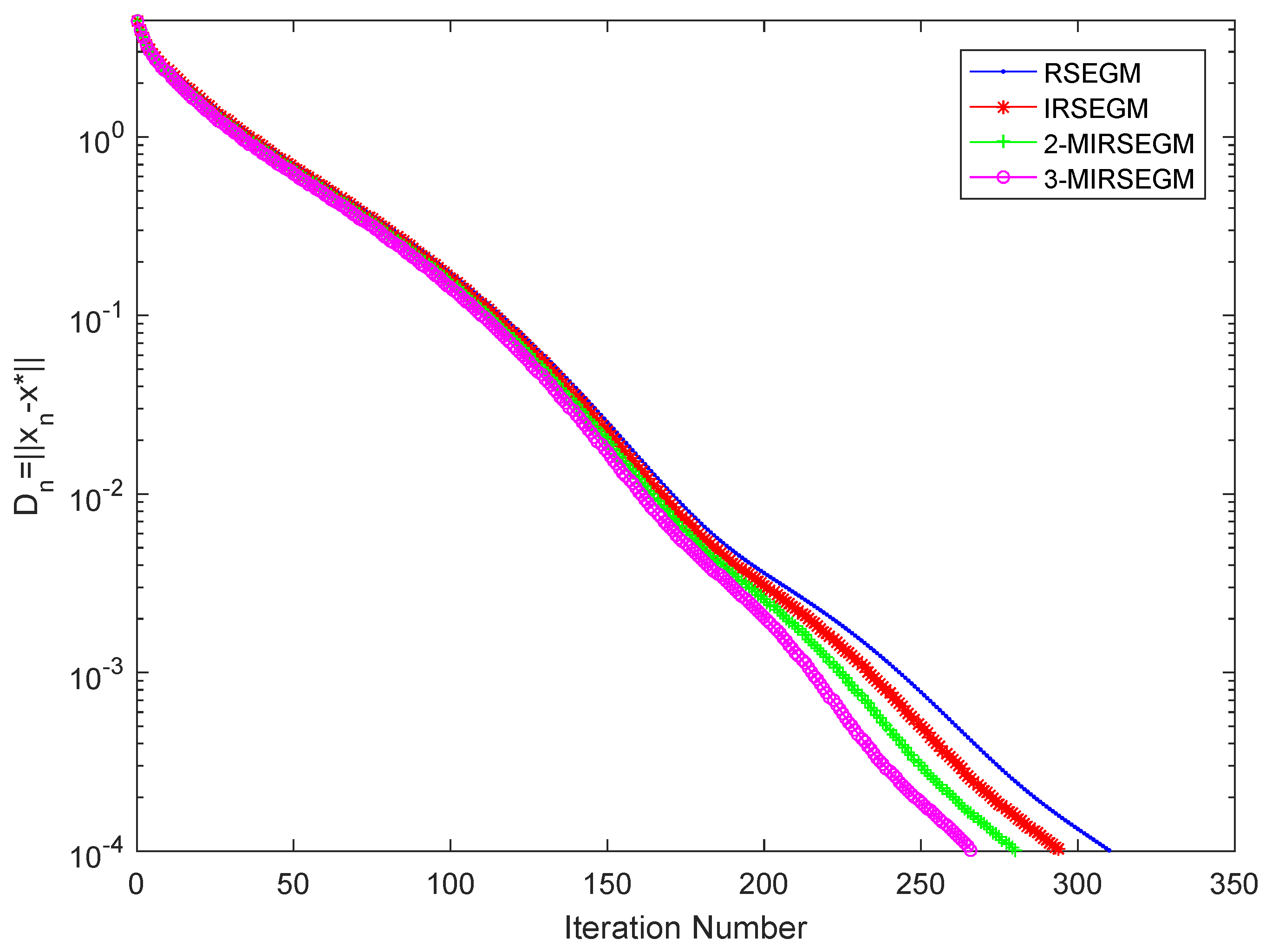
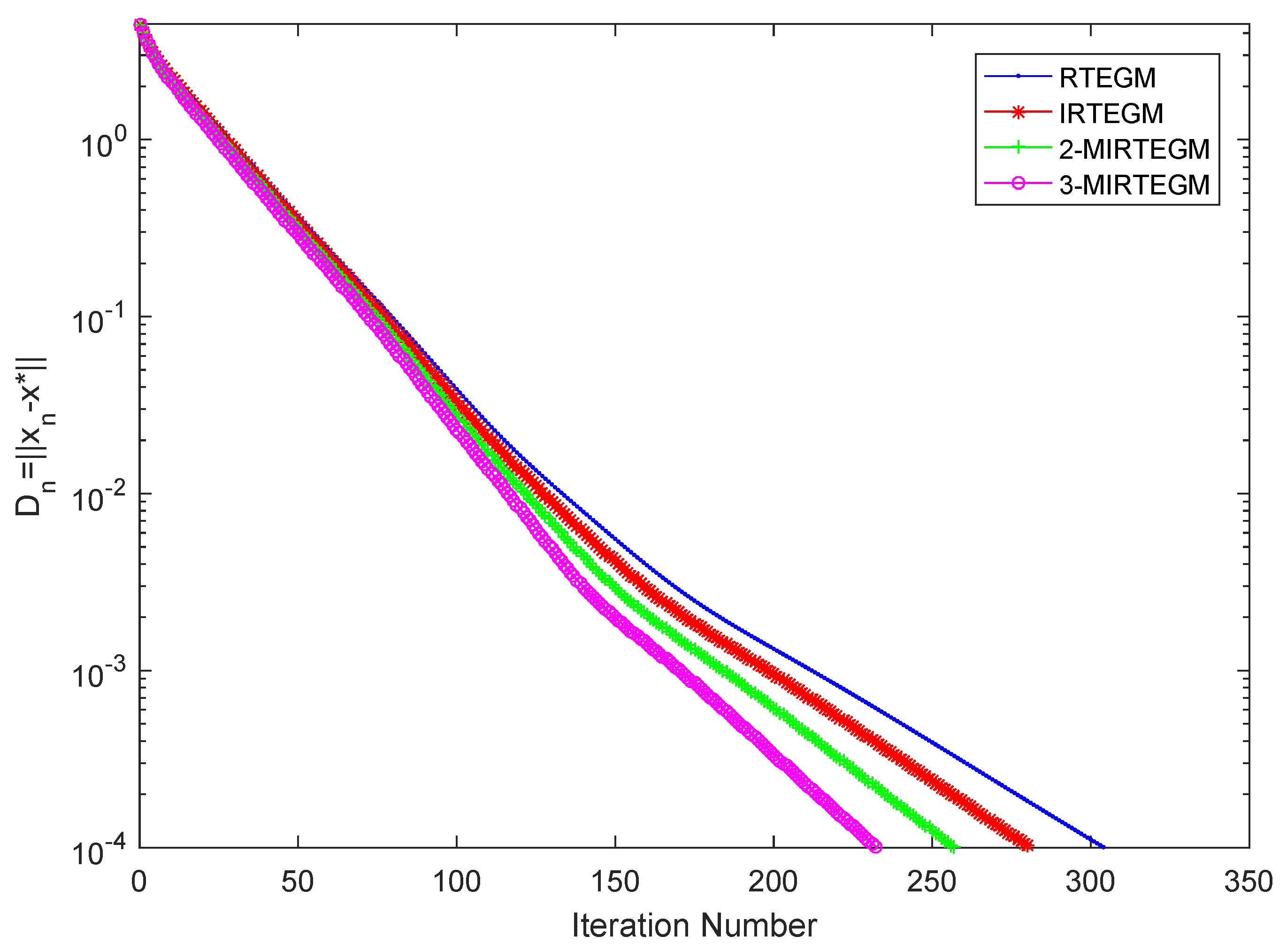
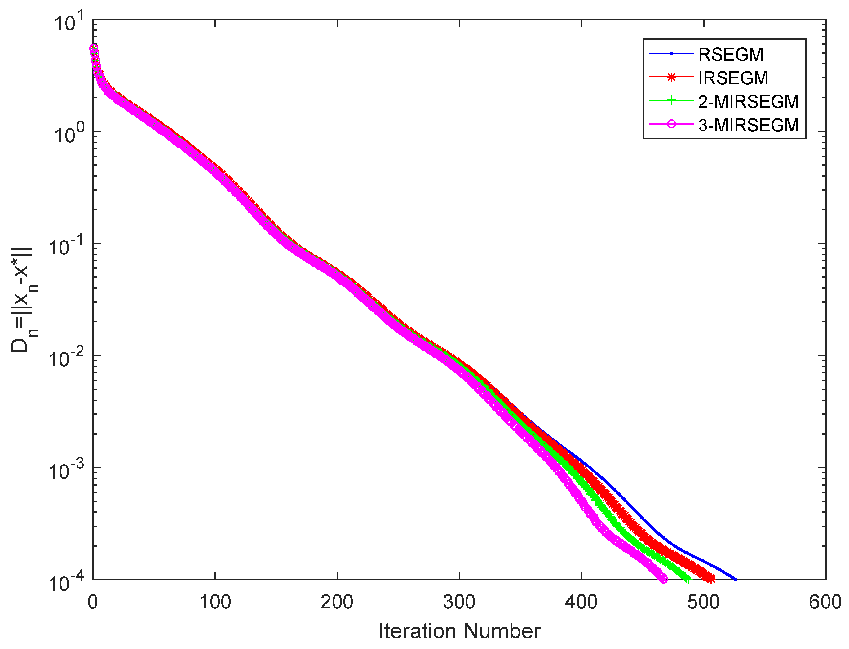
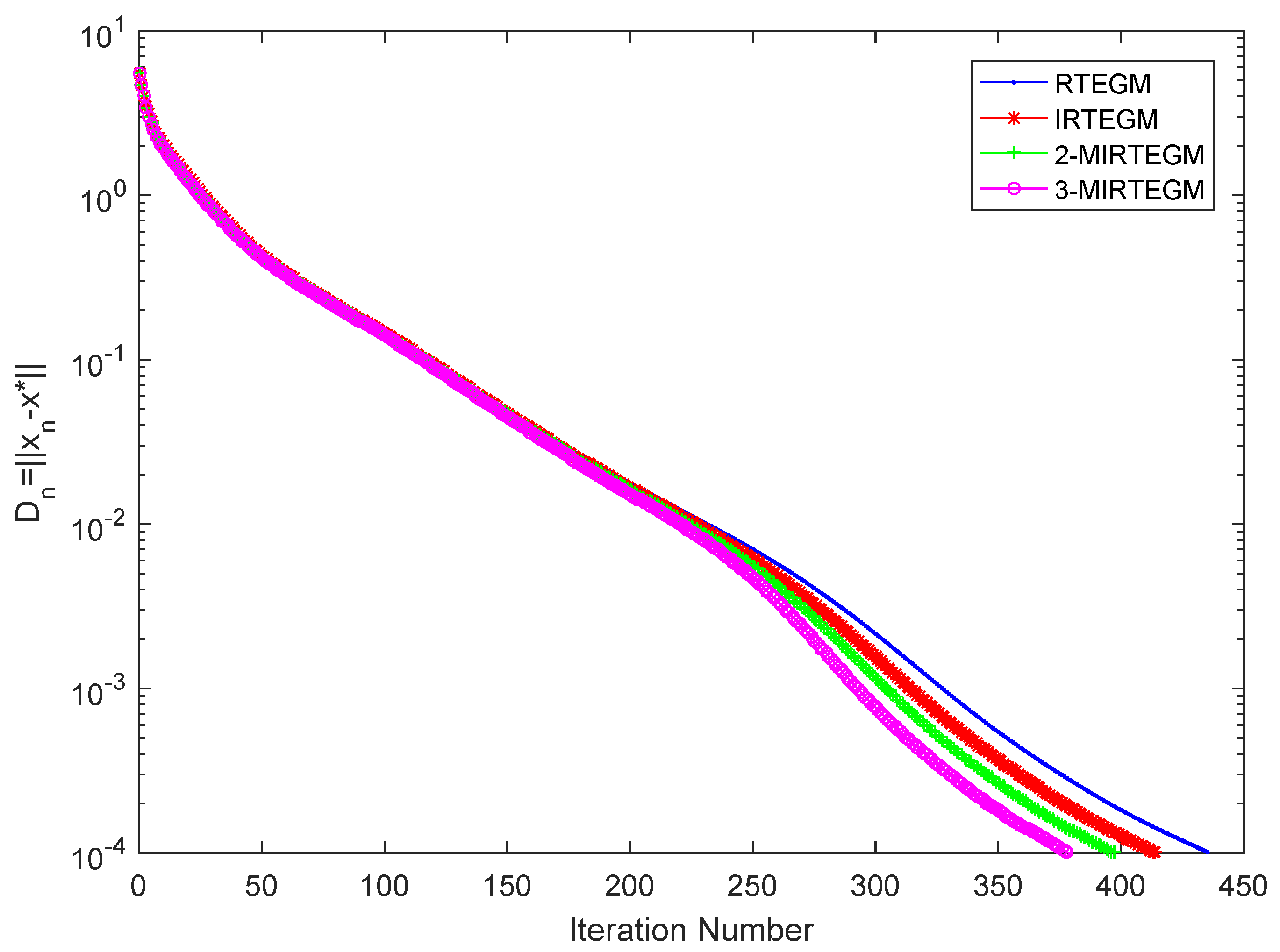
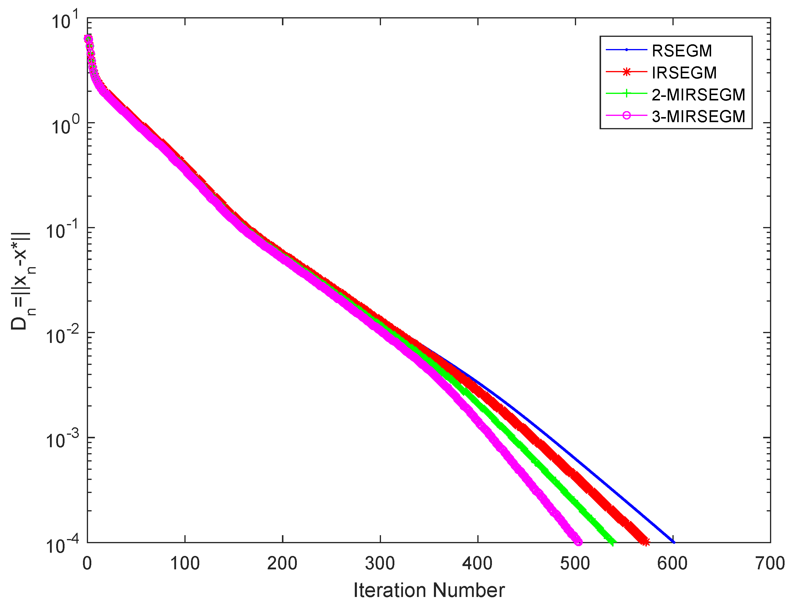
In this section, we give two numerical examples to illustrate the effectiveness and feasibility of our algorithms and compare with Algorithm 1 (RSEGM) and Algorithm 2 (RTEGM). We denote Algorithm 3 for , , by IRSEGM, 2-MIRSEGM and 3-MIRSEGM, respectively, denote Algorithm 4 for , , by IRTEGM, 2-MIRTEGM and 3-MIRTEGM, respectively. We write all the programmes in Matlab 9.0 and performed on PC Desktop Intel(R) Core(TM) i5-1035G1 CPU @ 1.00 GHz 1.19 GHz, RAM 16.0 GB.
Example 1. Let and . Let A be a function defined asfor each . It is easy to see that A is monotone and Lipschitz continuous. Let . Choose , and for IRSEGM, 2-MIRSEGM, 3-MIRSEGM, IRTEGM, 2-MIRTEGM and 3-MIRTEGM. Choose and for each algorithm. It is obvious that and hence is the unique solution of HVIP (4). We use for stopping criterion. We show the numerical results in Table 1 and Table 2. From these tables, we can easily see that the number of iterations of our algorithms is 10–40% less than RSEGM and RTEGM. Convergence of our algorithms is also much faster than RSEGM and RTEGM in term of elapsed time. Example 2. Let . We consider the HpHard problem [20,21]. Let be a mapping defined byfor each , where B is a matrix in , S is a skew-symmetric matrix in , D is a diagonal matrix in whose diagonal entries are positive, and is a vector. Thus, M is positive definite. Let C be a set defined by It is clear that A is monotone and Lipschitz continuous. Let . It is obvious that and hence is the unique solution of HVIP (1.6).
For the experiments, all the entries of B and S are generated randomly and uniformly in (−2,2), the diagonal entries of D are generated randomly and uniformly in (0,2), . We choose , and for IRSEGM, 2-MIRSEGM, 3-MIRSEGM, IRTEGM, 2-MIRTEGM and 3-MIRTEGM, choose , , and for each algorithm. We show the numerical results in Figure 1, Figure 2, Figure 3, Figure 4, Figure 5 and Figure 6. From these figures, we see that the algorithms we proposed have advantages over RSEGM and RTEGM. 6. Conclusions
In this paper, we constructed a multi-step inertial regularized subgradient extragradient method and a multi-step inertial Tseng’s extragradient method for solving HVIP (
6) in a Hilbert space when
F is a generalized Lipschitzian and hemicontinuous mapping, which are based on the multi-step inertial methods, Algorithm 1 (RSEGM) and Algorithm 2 (RTEGM). We presented two strong convergence theorems. Finally, we gave some numerical experiments to show the effectiveness and feasibility of our new iterative methods. From the numerical results, we can obviously see that our methods have advantages over Algorithms 1 and 2.
Our Algorithms 3 and 4 extend and improve Algorithms 1 and 2 in the following ways:
- (i)
The inertial method is used in Algorithms 3 and 4.
- (ii)
The Lipschitzian mapping F is generalized to a generalized Lipschitzian and hemicontinuous mapping.
In other words, if we let and L be a Lipschitzian mapping, then Algorithm 3 (or Algorithm 4) reduces to Algorithm 1 (or Algorithm 2).
Author Contributions
Conceptualization, J.-C.Y.; Data curation, B.J.; Formal analysis, Y.W.; Funding acquisition, Y.W. and J.-C.Y.; Investigation, B.J.; Methodology, B.J. and Y.W.; Resources, J.-C.Y.; Supervision, Y.W. and J.-C.Y.; Writing–original draft, B.J. All authors have read and agreed to the published version of the manuscript.
Funding
This research was funded by the National Natural Science Foundation of China, grant number 11671365.
Institutional Review Board Statement
Not applicable.
Informed Consent Statement
Not applicable.
Data Availability Statement
Not applicable.
Conflicts of Interest
The author declare that they have no competing interests.
References
- Tseng, P. A modified forward-backward splitting method for maximal monotone mappings. SIAM J. Control Optim. 2000, 38, 431–446. [Google Scholar] [CrossRef]
- Censor, Y.; Gibali, A.; Reich, S. The subgradient extragradient method for solving variational inequalities in Hilbert space. J. Optim. Theory Appl. 2011, 148, 318–335. [Google Scholar] [CrossRef] [PubMed] [Green Version]
- Hieu, D.V.; Muu, L.D.; Duong, H.N.; Thai, B.H. Strong convergence of new iterative projection methods with regularization for solving monotone variational inequalities in Hilbert spaces. Math. Meth. Appl. Sci. 2020, 43, 9745–9765. [Google Scholar] [CrossRef]
- Hieu, D.V.; Anh, P.K.; Muu, L.D. Strong convergence of subgradient extragradient method with regularization for solving variational inequalities. Optim. Eng. 2020. [Google Scholar] [CrossRef]
- Maingé, P.E. Inertial iterative process for fixed points of certain quasi-nonexpansive mapping. Set-Valued Anal. 2007, 15, 67–79. [Google Scholar] [CrossRef]
- Dong, Q.L.; Cho, Y.J.; Zhong, L.L.; Rassias, T.M. Inertial projection and contraction algorithms for variational inequalities. J. Glob. Optim. 2018, 70, 687–704. [Google Scholar] [CrossRef]
- Dong, Q.L.; Huang, J.Z.; Li, X.H.; Cho, Y.J.; Rassias, T.M. MiKM: Multi-step inertial Krasnosel’skiǐ–Mann algorithm and its applications. J. Glob. Optim. 2019, 73, 801–824. [Google Scholar] [CrossRef]
- Pan, C.; Wang, Y. Convergence theorems for modified inertial viscosity splitting methods in Banach spaces. Mathematics 2019, 7, 379. [Google Scholar] [CrossRef] [Green Version]
- Ceng, L.C.; Qin, X.; Shehu, Y.; Yao, J.C. Mildly inertial subgradient extragradient method for variational inequalities involving an asymptotically nonexpansive and finitely many nonexpansive mappings. Mathematics 2019, 7, 881. [Google Scholar] [CrossRef] [Green Version]
- Tian, M.; Jiang, B.N. Inertial Haugazeau’s hybrid subgradient extragradient algorithm for variational inequality problems in Banach spaces. Optimization 2021, 70, 987–1007. [Google Scholar] [CrossRef]
- Ceng, L.C.; Petruşel, A.; Qin, X.; Yao, J.C. Two inertial subgradient extragradient algorithms for variational inequalities with fixed-point constraints. Optimization 2021, 70, 1337–1358. [Google Scholar] [CrossRef]
- Shehu, Y.; Liu, L.; Mu, X.; Dong, Q.L. Analysis of versions of relaxed inertial projection and contraction method. Appl. Numer. Math. 2021, 165, 1–21. [Google Scholar] [CrossRef]
- Xu, H.K. Iterative methods for the split feasibility problem in infinite-dimensional Hilbert space. Inverse Probl. 2010, 26, 10518. [Google Scholar] [CrossRef]
- Zhou, H.; Zhou, Y.; Feng, G. Iterative methods for solving a class of monotone variational inequality problems with applications. J. Inequal. Appl. 2015, 2015, 68. [Google Scholar] [CrossRef] [Green Version]
- Kraikaew, R.; Saejung, S. Strong convergence of the Halpern subgradient extragradient method for solving variational inequalities in Hilbert spaces. J. Optim. Theory Appl. 2014, 163, 399–412. [Google Scholar] [CrossRef]
- Xu, H.K. Averaged mappings and the gradient-projection algorithm. J. Optim. Theory Appl. 2011, 150, 360–378. [Google Scholar] [CrossRef]
- Ceng, L.C.; Ansari, Q.H.; Yao, J.C. Some iterative methods for finding fixed points and for solving constrained convex minimization problems. Nonlinear Anal. 2011, 74, 5286–5302. [Google Scholar] [CrossRef]
- Liu, L.S. Ishikawa and Mann iterative process with errors for nonlinear strongly accretive mappings in Banach spaces. J. Math. Anal. Appl. 1995, 194, 114–125. [Google Scholar] [CrossRef] [Green Version]
- Xu, H.K. Iterative algorithms for nonlinear operators. J. Lond. Math. Soc. 2002, 66, 240–256. [Google Scholar] [CrossRef]
- Yang, J.; Liu, H. Strong convergence result for solving monotone variational inequalities in Hilbert space. Numer. Algorithm 2019, 80, 741–752. [Google Scholar] [CrossRef]
- Malitsky, Y.V. Projected reflected gradient methods for monotone variational inequalities. SIAM J. Optim. 2015, 25, 502–520. [Google Scholar] [CrossRef] [Green Version]
| Publisher’s Note: MDPI stays neutral with regard to jurisdictional claims in published maps and institutional affiliations. |
© 2021 by the authors. Licensee MDPI, Basel, Switzerland. This article is an open access article distributed under the terms and conditions of the Creative Commons Attribution (CC BY) license (https://creativecommons.org/licenses/by/4.0/).


