Marks: A New Interval Tool for Uncertainty, Vagueness and Indiscernibility

Abstract

The system of marks created by Dr. Ernest Gardenyes and Dr. Lambert Jorba was first published as a doctoral thesis in 2003 and then as a chapter in the book Modal Interval Analysis in 2014. Marks are presented as a tool to deal with uncertainties in physical quantities from measurements or calculations. When working with iterative processes, the slow convergence or the high number of simulation steps means that measurement errors and successive calculation errors can lead to a lack of significance in the results. In the system of marks, the validity of any computation results is explicit in their calculation. Thus, the mark acts as a safeguard, warning of such situations. Despite the obvious contribution that marks can make in the simulation, identification, and control of dynamical systems, some improvements are necessary for their practical application. This paper aims to present these improvements. In particular, a new, more efficient characterization of the difference operator and a new implementation of the marks library is presented. Examples in dynamical systems simulation, fault detection and control are also included to exemplify the practical use of the marks.

1. Introduction

Measurements of a variable are made using numerical scales. Usually, the value of a measurement is associated with a real number, but this association is not exact because of imperfect or partial knowledge due to uncertainty, vagueness or indiscernibility.

Incomplete knowledge comes from limited reliability of technical devices, partial knowledge, an insufficient number of observations, or other causes [1]. Among the different types of uncertainty, we find imprecision, vagueness, or indiscernibility. Vagueness, in the colloquial sense of the term, refers to ambiguity, which remains in a datum due to lack of precision, although its meaning is understood. An example could be the measurement of a person’s weight using a scale, which provides a value within a range of scale accuracy, e.g., between 75 and 75.2 kg. Uncertainty refers to imperfect or unknown information. For example, it is known that the weight of a car is within limits (1000–1500 kg), but the exact value is unknown due to missing information, such as the number of occupants and the load.

The problems of vagueness and uncertainty have received attention for long time by philosophers and logicians (e.g., [2,3]). Computational scientists have also provided new tools for dealing with uncertainty and vagueness, such as interval analysis, either classic intervals [4,5] or modal intervals [6,7], fuzzy set theory [8,9] and rough set theory [10].

Indiscernibility has also received the attention of philosophers. The identity of indiscernible [11] states is that no two distinct things are exactly alike. It is often referred to as “Leibniz’s Law” and is usually understood to mean that no two objects have exactly the same properties. The identity of indiscernibility is interesting because it raises questions about the factors that individuate qualitatively identical objects. The marks, which are presented and developed in this paper, are outlined to address indiscernibility.

For example, the temperature in a room can be measured with a thermometer at different location points within the room to obtain a spatial distribution. So the temperature is not, for example, 20 °C but an interval of values, between, for example 19 and 21 that represents the different values of the temperature in the room. It does not represent the temperature of the room, which might be necessary for the modeling of an air-conditioning system. The temperature is at this time one value of the interval [19,21], considering the points of this interval as being indistinguishable. This is a known issue in handling “lumped” or “distributed” quantities. Moreover, the thermometer used as a measurement device has a specific precision and provides a reading on a specific scale, which is likely translated to another digital scale to be used in computations. Therefore, a real number or even an interval is not able to represent the read temperature.

Until the 20th century, the preferred theory for modeling uncertainty was probability theory [12], but the introduction of fuzzy sets by Zadeh [8] had a profound impact on the notion of uncertainty. At present, sources of uncertainty remain an active challenge for the scientific community, and different research efforts are directed toward finding solutions to deal with these uncertainties, such as using Bayesian inference for predictions of turbulent flows in aerospace engineering [13], fuzzy sets for time series forecasting based on particle swarm optimization techniques [14], modal intervals for prediction modeling in grammatical evolution [15], interval analysis method based on Taylor expansion for distributed dynamic load identification [16] or rough sets to evaluate the indoor air quality [17].

In this article, marks are presented as a framework to deal with quantities represented in digital scales because this methodology can take into account many the sources of uncertainty. In any use of a mathematical model of a physical system, such as simulation, fault detection, or control, the system of marks provides values for the state variables and, simultaneously, their corresponding granularities, which represent a measure of the accumulated errors in the successive computations. This performance leads to the following:

• Define intervals of variation for these variables values.
• Decide the valid values, i.e., which have a meaning, provide by the semantic theorem.
• Warns from which simulation step the obtained values will be meaningless because the granularity is greater than the previously fixed tolerance.

In the following sections of this paper, we present and review marks theory and basic arithmetic operations. The main contributions of this paper are the following:

• A new characterization for the difference operator;
• A new characterization for the difference operator;
• A new implementation of the marks library and software developments that are needed to apply these methodologies.

To demonstrate the applicability and potential of marks, a well-known benchmark in process control in which the problems of uncertainty, imprecision, and indiscernibility are present is introduced. After introducing the benchmark, three different problems built on it are presented and solved, using marks: simulation, fault detection, and control.

2. Marks

An approach to deal with the inaccuracy associated with any measurement or computation process with physical quantities is built by means of an interval tool: marks, which define intervals in which it is not possible to make any distinction between its elements, i.e., indiscernibility intervals. Marks are computational objects; however, initial marks can come from either direct or indirect readings from a measurement device. Therefore, it is necessary to represent them on a computational scale to acquire suitable computation items. When a measurement reading or a computation is obtained as a number on a numerical scale, the resulting value has to be associated to a subset of R of indiscernible numbers from this value. Each point of this subset has the same right to be considered as the value of the measurement or computation. This kind of subsets leads to the concept of a mark considered a “spot” of certain size, called the “granularity” of the mark.

Let $D{I}_n$ be a digital scale in floating point notation. A mark on $D{I}_n$ is a tuple of the following five real numbers:

• Center: a number c on the digital scale, which is the reading of the mark on $D{I}_n$.
• Number of digits: the number of digits n on the digital scale $D{I}_n$, $n=15$ computing in double precision.
• Base: the $base$ of the number system b, usually $b=10$.
• Tolerance: an uncertainty that expresses the relative separation among the points of the scale that the observer considers as indiscernible from the center. It is a relative value greater or equal than $b^{-n}$, which is the minimum computational error on the digital scales. It is a measure to decide if the mark is to be accepted as valid.
• Granularity: an error g, coming from the inaccurate measure or computation, which will increase in every computational process. It must include the imprecision of the measure, devices calibration errors, inaccuracy of the physical system concerned, etc., and it is always expressed in relative terms, i.e., a number between 0 and 1, less than tolerance.

As the numbers n and b are specific on the digital scale $D{I}_n$, and the value of the tolerance t is assigned for the user, the mark will be denoted by $\mathfrak{m}=\langle c,g\rangle$. Tolerance t, number of digits n and base b define the $type$ of the mark. The set of marks of the same type is denoted by $M(t,n,b)$.

The center of a mark is a reading in a measurement device, so it carries an error and an uncertainty associated to the problem under study. Both yield the value of its granularity. The center and granularity define the mark on the digital scale. Now, it is possible to start the computations required by the mathematical model. The errors in each step of the computations will increase the value of the granularity.

The granularity and tolerance must satisfy a minimum condition of validity of the mark as follows:

$$b^{-n}\le g<t<1,$$

(1)

These concepts are developed in [7,18], which contain the definition of a mark, its components (center, tolerance, granularity, and base number of the numerical scale), features (valid or invalid mark and associated intervals), relationships (equality and inequality), basic operators (max, min, sum, difference, product, and quotient) and general functions of marks and semantic interpretations through associated intervals to the operands and the results.

2.1. Basic Operators of Marks

Operations between marks are defined for marks of the same type and the result is also of the same type as the data. In this way, the tolerance is constant along with any computation, but the granularity increases, reflecting the step-by-step loss of information, which constitutes the deviation of the computed value from the exact value. An extract definition of elementary operators is presented after this, together with a different characterization of the operator difference.

The extension $f_M$ of a basic operator $f\in \{max,min,+,-,\ast ,/\}$ to two given marks $\mathfrak{x}=\langle c_x,g_x\rangle \in M(t,n,b)$ and $\mathfrak{y}=\langle c_y,g_y\rangle \in M(t,n,b)$ is the following:

$$\begin{array}{c}\hfill f_M(\mathfrak{x},\mathfrak{y})=\langle di(f(c_x,c_y),g_z\rangle \in M(t,n,b)\end{array}$$

where $di\left(f(c_x,c_y)\right)$ is the digital computation of the function f at $(c_x,c_y)$ on the scale ${DI}_n$, supposing a minimum relative displacement of $di\left(f(c_x,c_y)\right)$ with regard to the exact value $f(c_x,c_y)$; and $g_z$ is the granularity of the result, which has to be $g_z\ge max(g_x,g_y)$ and is specified as the following:

$$g_z={\gamma }_{x,y}+b^{-n}$$

where the value $b^{-n}$ is the computation error of $di\left(f(c_x,c_y)\right)$, which is the minimum error of any computation. Any computation has to carry this error by adding $b^{-n}$. The term ${\gamma }_{x,y}$ is the smallest number, verifying the following:

$$\begin{array}{c}f(c_x,c_y)\ast [1+{\gamma }_{x,y},1-{\gamma }_{x,y}]\subseteq fR(c_x\ast [1+g_x,1-g_x],c_y)\hfill \\ f(c_x,c_y)\ast [1+{\gamma }_{x,y},1-{\gamma }_{x,y}]\subseteq fR(c_x,c_y\ast [1+g_y,1-g_y])\hfill \end{array}$$

where $fR$ is the modal syntactic extension of f [7].

For the operators min and max, no computations with the centers are necessary and the resulting granularity is $g_z=max(g_x,g_y)$. The results are transformed to the following:

$$\begin{array}{c}max\{\mathfrak{x},\mathfrak{y}\}=\langle max\{c_x,c_y\},max\{g_x,g_y\}\rangle \hfill \end{array}$$

(2)

$$\begin{array}{c}min\{\mathfrak{x},\mathfrak{y}\}=\langle min\{c_x,c_y\},max\{g_x,g_y\}\rangle \hfill \end{array}$$

(3)

$$\begin{array}{c}\mathfrak{x}+\mathfrak{y}=\langle c_x+c_y,max\{g_x,g_y\}+b^{-n}\rangle \hfill \end{array}$$

(4)

$$\begin{array}{c}\mathfrak{x}-\mathfrak{y}=\left\{\begin{array}{cc}\langle c_x-c_y,max\left\{g_x,g_y,\left|\frac{|c_x|}{|c_x|-|c_y|}\right|g_x,\left|\frac{|c_y|}{|c_x|-|c_y|}\right|g_y\right\}+b^{-n}\rangle & \mathrm{if}{c}_x\ne c_y\\ \langle 0,max\left\{g_x,g_y\right\}\rangle & \mathrm{if}{c}_x=c_y\end{array}\right.\hfill \end{array}$$

(5)

$$\begin{array}{c}\mathfrak{x}\ast \mathfrak{y}=\langle c_x\ast c_y,max\{g_x,g_y\}+b^{-n}\rangle \hfill \end{array}$$

(6)

$$\begin{array}{c}\mathfrak{x}/\mathfrak{y}=\langle c_x/c_y,max\left\{g_x,\frac{g_y}{1-g_y}\right\}+b^{-n}\rangle \hfill \end{array}$$

(7)

where $c_x$ and $c_y$ are think positive for the operators + and −.

The difference in the particular case of two marks with equal centers is 0 without any computation. There is a similar situation with the maximum and minimum operators. In these cases, the granularity of the result must be the greatest of the operands’ granularities.

Two shortcomings in the use of marks as numerical entities are evident. The first one concerns the granularity of the difference between two marks $\mathfrak{x}$ and $\mathfrak{y}$ with positive but near centers. In its formula, the difference between the two centers appears as the denominator in a fraction. Consequently, when the centers are close, the granularity can be large enough to invalidate the mark, i.e., when granularity is larger than the tolerance, thus invalidating any further result. This can be avoided by taking into account the two real numbers x and y:

$$x-y=\frac{x^m-y^m}{x^{m-1}\ast y^0+x^{m-2}\ast y^1+\dots +x^1\ast y^{m-2}+x^0\ast y^{m-1}},$$

hence, it is possible to compute the difference $\mathfrak{x}-\mathfrak{y}$ as the following:

$$\mathfrak{x}-\mathfrak{y}=({\mathfrak{x}}^m-{\mathfrak{y}}^m)/({\mathfrak{x}}^{m-1}\ast {\mathfrak{y}}^0+{\mathfrak{x}}^{m-2}\ast \mathfrak{y}+\dots +\mathfrak{x}\ast {\mathfrak{y}}^{m-2}+{\mathfrak{x}}^0\ast {\mathfrak{y}}^{m-1})$$

(8)

where m is a natural number large enough so that ${\mathfrak{x}}^m$ and ${\mathfrak{y}}^m$ are not near. The center of the resulting mark is $c_x-c_y$, but its granularity is both different and lesser.

Firstly, to avoid overflows in the computations of ${\mathfrak{x}}^m$ and ${\mathfrak{y}}^m$ it is convenient to normalize, a priori, the two marks to be divided by the greater mark $\mathfrak{m}=max(\mathfrak{x},\mathfrak{y})$. For example, if, $c_y<c_x$ then, $\mathfrak{m}=\mathfrak{x}$, and the normalized marks are the following:

$$\mathfrak{u}=\mathfrak{x}/\mathfrak{m}=\langle 1,g_u\rangle ,\mathfrak{v}=\mathfrak{y}/\mathfrak{m}=\langle c,g_v\rangle ,$$

with $0<c<1$, and the difference is at this time the following:

$$\mathfrak{u}-\mathfrak{v}=({\mathfrak{u}}^m-{\mathfrak{v}}^m)/({\mathfrak{u}}^{m-1}\ast {\mathfrak{v}}^0+{\mathfrak{u}}^{m-2}\ast \mathfrak{v}+\dots +\mathfrak{u}\ast {\mathfrak{v}}^{m-2}+{\mathfrak{u}}^0\ast {\mathfrak{v}}^{m-1}).$$

(9)

The power of one mark ${\langle c_x,g_x\rangle }^m$ with m a natural number is a particular case of a product with the same factors ${\langle c_x,g_x\rangle }^m=\langle c_x,g_x\rangle \ast \cdots \ast \langle c_x,g_x\rangle$ then, by induction it is the following:

$${\langle c_x,g_x\rangle }^m=\langle c_x^m,g_x+(m-1)b^{-n}\rangle .$$

Then, the numerator of (9) is as follows:

$$\mathfrak{N}={\mathfrak{u}}^m-{\mathfrak{v}}^m=\langle 1,(g_u+(m-1)b^{-n}\rangle -\langle c^m,g_v+(m-1)b^{-n}\rangle$$

and can be calculated by means of the former formula (5). If $c^m\le 1/2$, then the following holds:

$$\mathfrak{N}=\langle 1-c^m,max((g_u+(m-1)b^{-n})/(1-c^m),g_v+(m-1)b^{-n})\rangle ,$$

(10)

interchanging $g_u$ and $g_v$ when $c_x<c_y$.

$\mathfrak{N}$ will be a valid mark when its granularity is small, i.e., when the term $c^m$ is less than a fixed small number $ϵ<1/2$, for example $ϵ=b^{-n}$. So,

$$m=[log\left(b^{-n}\right)/log\left(c\right)].$$

(11)

The computation of the denominator of the Equation (9) is not problematic because all their terms are positive:

$$\begin{array}{ccc}& & {\mathfrak{u}}^{m-1}=\langle 1,max(g_u+(m-2)b^{-n}\rangle \hfill \\ & & {\mathfrak{u}}^{m-2}\ast {\mathfrak{v}}^1=\langle c,max(g_u+(m-3)b^{-n},g_v)+b^{-n}\rangle =\hfill \\ & & =\langle c,max(g_u+(m-2)b^{-n},g_v+b^{-n})\rangle \hfill \\ & & \cdots \cdots \cdots \cdots \cdots \cdots \cdots \cdots \cdots \cdots \cdots \cdots \cdots \cdots \hfill \\ & & {\mathfrak{u}}^{m-i}\ast {\mathfrak{v}}^{i-1}=\langle c^{i-1},max(g_u+(m+i-1)b^{-n},g_v+(i-2)\ast b^{-n})+b^{-n}\rangle \hfill \\ & & =\langle c^{i-1},max(g_u+(m-i)b^{-n},g_v+(i-1)b^{-n})\rangle \hfill \\ & & \cdots \cdots \cdots \cdots \cdots \cdots \cdots \cdots \cdots \cdots \cdots \cdots \cdots \cdots \hfill \\ & & {\mathfrak{u}}^1\ast {\mathfrak{v}}^{m-2}=\langle c^{m-2},max(g_u,g_v+(m-3)b^{-n})+b^{-n}\rangle =\hfill \\ & & =\langle c^{m-2},max(g_u+b^{-n},g_v+(m-2)b^{-n})\rangle \hfill \\ & & {\mathfrak{v}}^{m-1}=\langle c^{m-1},g_v+(m-1)b^{-n})\hfill \end{array}$$

it results to

$$\mathfrak{D}=\langle (1^m-c^m)/(1-c),max(g_u+m{b}^{-n},g_v+(2m-1)b^{-n})\rangle .$$

(12)

Dividing $\mathfrak{N}$ and $\mathfrak{D}$

$$\mathfrak{u}-\mathfrak{v}=\mathfrak{N}/\mathfrak{D}$$

and, eventually de-normalizing by multiplying by $\mathfrak{m}$,

$$\mathfrak{x}-\mathfrak{y}=(\mathfrak{u}-\mathfrak{v})\ast \mathfrak{m}.$$

(13)

For example, for $t=0.05$, $b=10$, $n=15$, the formula (5) gives the following:

$$\langle 3.121,0.0001\rangle -\langle 3.1212,0.0001\rangle =\langle -0.0002,1.560600\rangle ,$$

which is an invalid mark because the granularity is larger than 1. From (11), $m=538995$ and (13) give the following:

$$\langle 3.121,0.0001\rangle -\langle 3.1212,0.0001\rangle =\langle -0.0002,0.010101\rangle ,$$

a valid mark.

The second shortcoming is the necessity to calculate the elementary functions (exp, log, power, trigonometric,…) for marks. This is possible with power series but when the convergence is slow, run time can belong. A better alternative is to use the routines ©FDLIBM developed at SunSoft, Sun Microsystems, to approximate these functions using polynomials. The computational processes for marks were developed and integrated into MATLAB in the MICELab research group (Institute of Informatics and Applications, University of Girona). The code to perform computations with marks can be found in [19].

2.2. Associated Intervals

The theory of marks is a by-product of modal intervals theory, linked by the “improper” [7] associated interval to a mark denoted by $Iv\left(\mathfrak{m}\right)$:

$$Iv\left(\mathfrak{m}\right)=c\ast [1+t,1-t],$$

(14)

where * is the product of a real number by an interval. Its domain, or set of its points, is referred to as $I{v}^{\prime }$ and called the indiscernibility margin of $\mathfrak{m}$. Another related interval is the external shadow defined by the following:

$$Exsh\left(\mathfrak{m}\right)=Iv\left(\mathfrak{m}\right)\ast [1-g,1+g]=c\ast [1+t,1-t]\ast [1-g,1+g],$$

(15)

necessary to obtain the semantic meaning of a computation made using marks. As $g<t$, the external shadow is an improper interval that verifies the inclusion of $Exsh\left(\mathfrak{m}\right)\subseteq Iv\left(\mathfrak{m}\right)$.

2.3. Semantic Theorem for Marks

The associated intervals allow the semantic properties of Modal Intervals to be applied to the results of functions of marks. Given the marks ${\mathfrak{x}}_1,\dots ,{\mathfrak{x}}_n\in M(t,b,n)$, the continuous ${\mathbb{R}}^n$ to $\mathbb{R}$ function $z=f(x_1,\dots ,x_n)$ and the modal syntactic extension $fR$ of f, then the following holds:

$$fR(Iv\left({\mathfrak{x}}_1\right),\dots ,Iv\left({\mathfrak{x}}_n\right))\subseteq Exsh\left(\mathfrak{z}\right).$$

This inclusion confirms the important Semantic Theorem for a function of marks, which provides meaning to any valid result in the evaluation of a function. If the mark $\mathfrak{z}$ is the calculus of a function of marks, $\mathfrak{z}=f_M({\mathfrak{x}}_1,\dots ,{\mathfrak{x}}_k)$, supposing that all the involved marks are valid, then we have the following:

$$(\forall z\in Exs{h}^{\prime }\left(\mathfrak{z}\right))(\exists x_1\in I{v}^{\prime }\left({\mathfrak{x}}_1\right))\dots (\exists x_k\in I{v}^{\prime }\left({\mathfrak{x}}_n\right))z=f(x_1,\dots ,x_n).$$

(16)

So, every point of the external shadow $Exs{h}^{\prime }\left(\mathfrak{z}\right)$ is a true value of the function f for some values of the variables in the intervals $I{v}^{\prime }\left({\mathfrak{x}}_1\right)\dots I{v}^{\prime }\left({\mathfrak{x}}_n\right)$.

The external shadow interval depends on the tolerance and the granularity of the mark, which shrinks the interval width with the unavoidable increase of the granularity. As the value approaches the tolerance (the center), the interval width tends to zero. This effect causes a loss of significance, which in many cases, is possible to avoid by performing a “translation” to avoid small values of the state variables. For example, adding a constant to the values of the state variables and scaling the common tolerance, if it depends on these values.

3. Benchmark

3.1. Benchmark Description

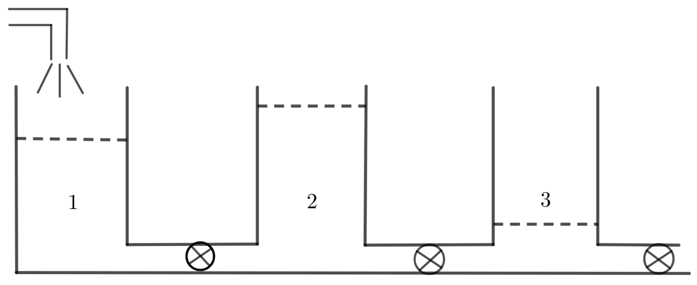
The popular three-tank benchmark problem is used to exemplify the usefulness of marks in the context of uncertainty, vagueness, and indiscernibility [20,21]. It consists of three cylindrical tanks of liquid connected by pipes of circular section, as depicted in Figure 1. The first tank has an incoming flow, which can be controlled using a pump (actuator) and the outflow is located in the last tank.

The model in form of difference equations for this systems is

$$\begin{array}{ccc}\hfill & & h_1(t+1)=h_1\left(t\right)+\Delta t·(q_1\left(t\right)-c_{12}·sr{h}_{12}·c{c}_1)/s_1\hfill \\ \hfill & & h_2(t+1)=h_2\left(t\right)+\Delta t·(q_2\left(t\right)+c_{12}·sr{h}_{12}·c{c}_1-c_{23}·sr{h}_{23}·c{c}_2)/s_1\hfill \\ & & h_3(t+1)=h_3\left(t\right)+\Delta t·(q_3\left(t\right)+c_{23}·sr{h}_{23}·c{c}_2-c_{30}·sr{h}_{30}·c{c}_3)/s_3\hfill \\ & & \mathrm{with}\hfill \\ & & sr{h}_{12}=\mathrm{sign}(h_1\left(t\right)-h_2\left(t\right))·\sqrt{|h_1\left(t\right)-h_2\left(t\right)|}\hfill \\ & & sr{h}_{23}=\mathrm{sign}(h_2\left(t\right)-h_3\left(t\right))·\sqrt{|h_2\left(t\right)-h_3\left(t\right)|}\hfill \\ & & sr{h}_{30}=\mathrm{sign}(h_3\left(t\right)-0)·\sqrt{|h_3\left(t\right)-0|}\hfill \end{array}$$

(17)

where the state variables $h_1$, $h_2$, $h_3$ are the level of liquid in the tanks, $s_1$, $s_2$, $s_3$ their respective areas, $q_1$, $q_2$, $q_3$ the incoming flows, $c_{12}$, $c_{23}$, $c_{30}$ the valves constants which represent the flux between the tanks and $\Delta t$ is the simulation step, in seconds.

The following values were considered: the three tanks are the same heights $h=2$ m, areas $s_1=s_2=s_3=1$ m${}^2$, and intermittent inputs of the maximum incoming flows (in m${}^3$/s) are the following:

$$q_1=0.01,q_2=q_3=0.$$

(18)

For the valves’ constants (in m${}^{5/2}$/s) the values are

$$c_{12}=0.009,c_{23}=0.008,c_{30}=0.007$$

(19)

and the initial liquid levels (in m) are

$$h_1\left(0\right)=0.1,h_2\left(0\right)=1.5,h_3\left(0\right)=0.6.$$

(20)

As an example of the application of marks for this benchmark model, we present three general problems related to many mathematical models: simulation, fault detection, and control to show the suitability of the marks for dealing with mathematical models with uncertainty and indiscernibility.

3.2. Simulation

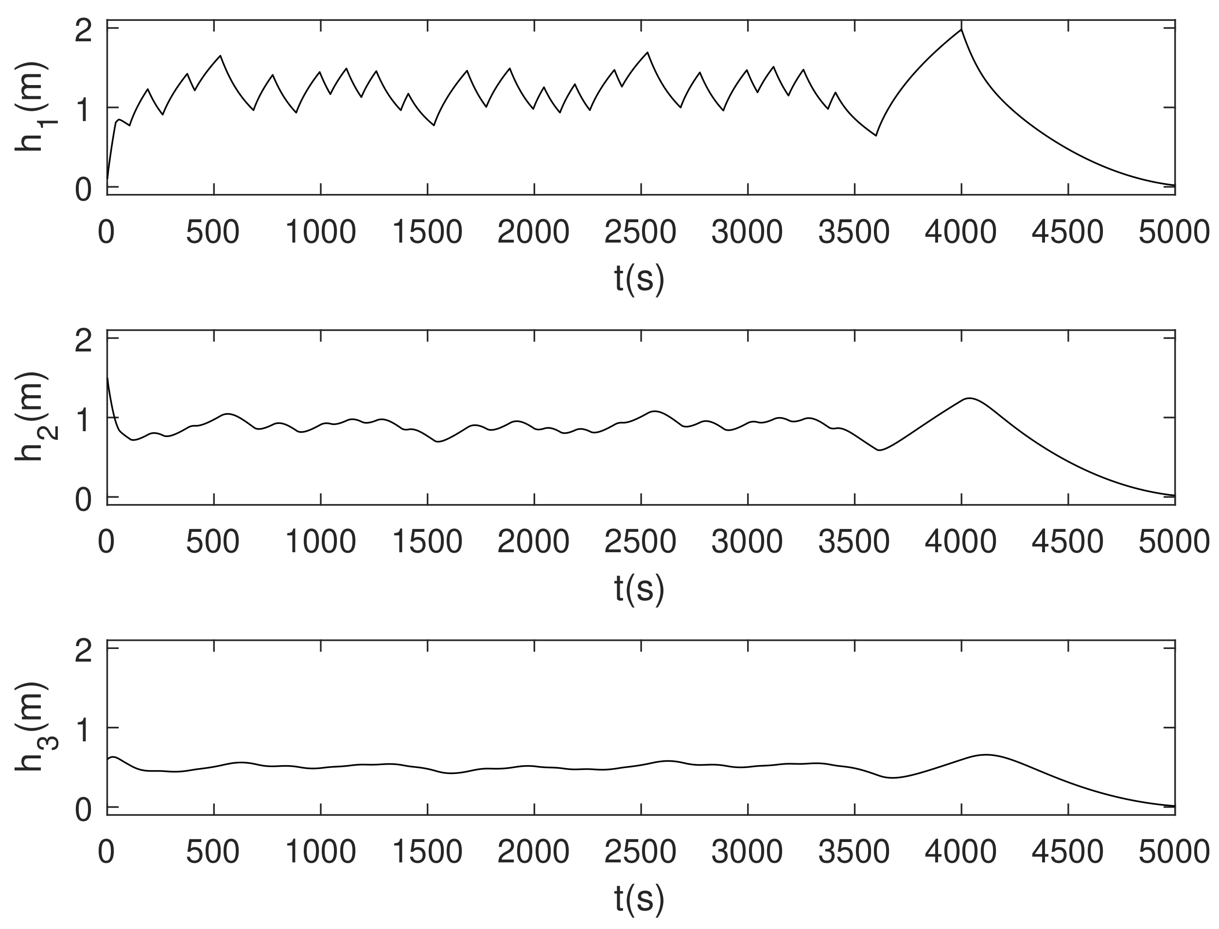
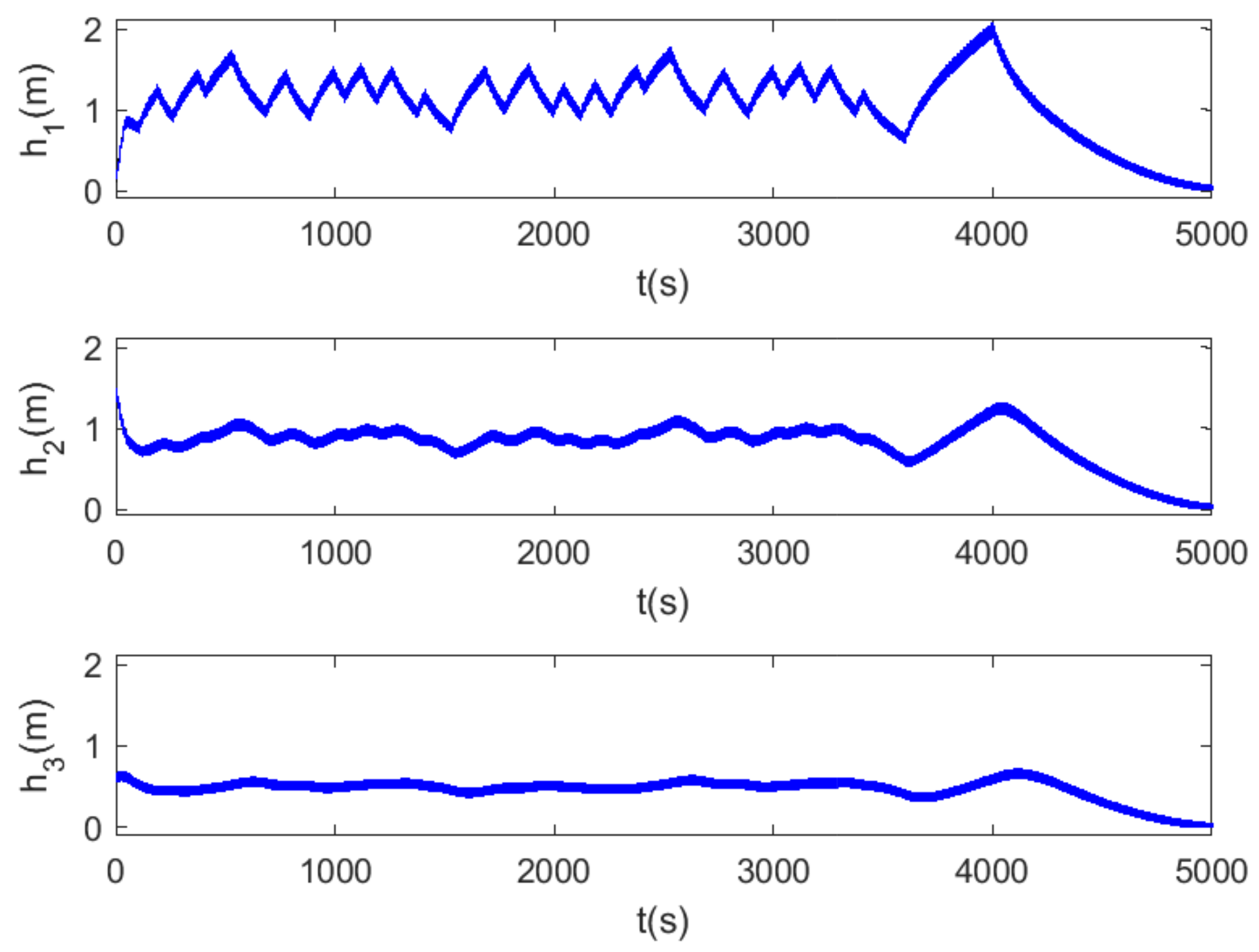
Two different types of simulations have been performed: using real numbers and using marks, with a simulation step of $\Delta t=5$ and 1000 steps of simulations (5000 s in all). The results using real numbers, for the three state variables are represented in Figure 2. The intermittent input flow gives the sawtooth shape for the values of $h_1$.

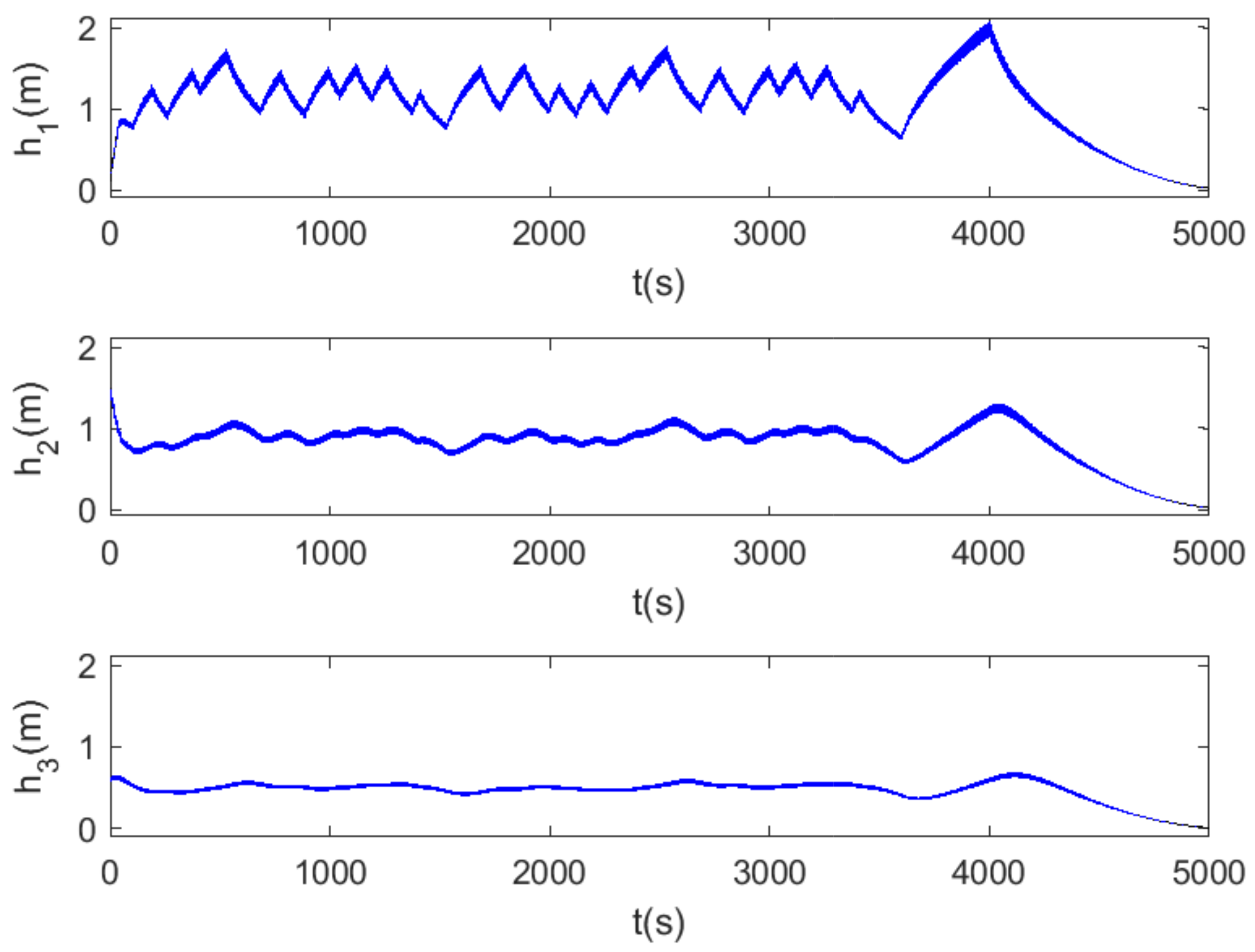
For the simulations using marks, all magnitudes are considered as marks whose centers are the former real numbers and granularities have been fixed to $g=0.00001$, for all the marks. The levels of liquid into the tanks are influenced by perturbations and the dynamics of the inputs and outputs of liquid. Calling $pr$ this variation, the tolerance can be calculated by $t=pr/h$. Taking $pr=0.10$, the common tolerance for all the simulations is $t=0.05$. Unlike the granularities, the tolerances have to be equal for all the marks.

Results are shown in Figure 3 that contains the intervals associated to the marks, drawn in form of little vertical segments. Together, they are represented by the dark band of the figure. The run time for the $t=5000$ s of the simulation is 200 s.

In accordance with the semantic of marks (16) these results mean that, for one instant, for example $i=500$ (time $t=2500$ s), the model outputs the result in these marks and related associated intervals:

$$\begin{array}{ccc}& & {\mathfrak{h}}_1\left(2500\right)=\langle 1.588474,0.000011\rangle ,I{v}^{\prime }\left({\mathfrak{h}}_1\left(2500\right)\right)=[1.509068,1.667881]\hfill \\ & & {\mathfrak{h}}_2\left(2500\right)=\langle 1.003461,0.000011\rangle ,I{v}^{\prime }\left({\mathfrak{h}}_2\left(2500\right)\right)=[0.953299,1.053623]\hfill \\ & & {\mathfrak{h}}_3\left(2500\right)=\langle 0.525883,0.000011\rangle ,I{v}^{\prime }\left({\mathfrak{h}}_3\left(2500\right)\right)=[0.499595,0.552171].\hfill \end{array}$$

An experimental state value like

$$\begin{array}{ccc}\hfill h_{1exp}\left(2500\right)& =& 1.6\pm 0.01\mathrm{m},\hfill \\ \hfill h_{2exp}\left(2500\right)& =& 1\pm 0.01\mathrm{m},\hfill \\ \hfill h_{3exp}\left(2500\right)& =& 0.52\pm 0.01\mathrm{m}.\hfill \end{array}$$

is contained in them and, thus, consistent with the model (17).

However, for $t=5000$ s the results are the following:

$$\begin{array}{ccc}& & {\mathfrak{h}}_1\left(5000\right)=\langle 0.018793,0.000011\rangle ,I{v}^{\prime }\left({\mathfrak{h}}_1\left(5000\right)\right)=[0.017854,0.019733]\hfill \\ & & {\mathfrak{h}}_2\left(5000\right)=\langle 0.017685,0.000011\rangle ,I{v}^{\prime }\left({\mathfrak{h}}_2\left(5000\right)\right)=[0.016801,0.018569]\hfill \\ & & {\mathfrak{h}}_3\left(5000\right)=\langle 0.012397,0.000011\rangle ,I{v}^{\prime }\left({\mathfrak{h}}_3\left(5000\right)\right)=[0.011778,0.013017].\hfill \end{array}$$

with the associated intervals too narrow to obtain reasonable results with the related semantic (16).

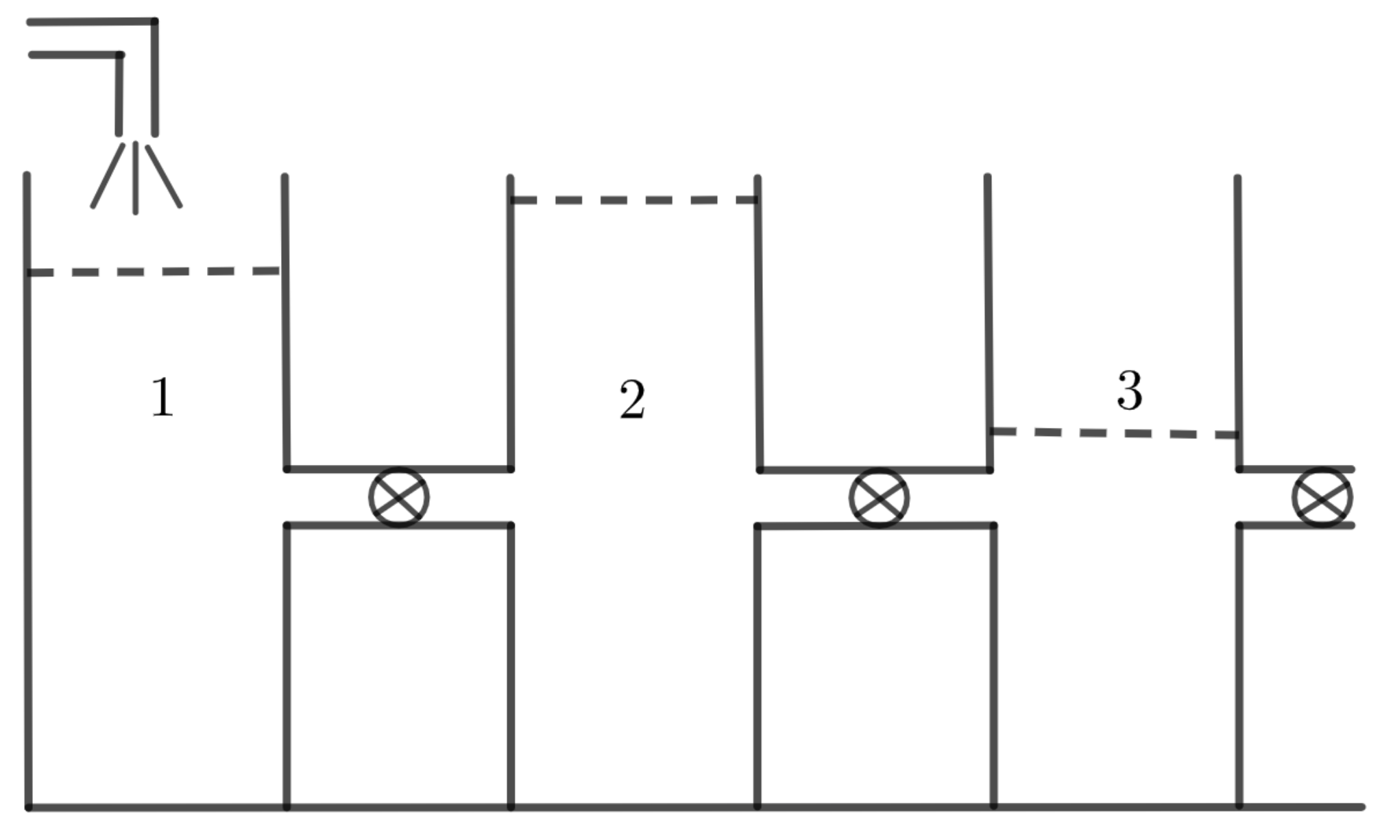
The heights values contained in the associated intervals (14) are consistent with the model, but these intervals depend on the value of the center of the mark because their widths tend to zero, as shown in the final parts of the graphics in Figure 3. To avoid this effect, in this benchmark, it is possible to change to a physical system (Figure 4), where the common height of the tanks is $h+h_{exc}$. The behaviour of the liquid levels along the simulations is the same for the two physical systems.

To do this in the simulation algorithm, it is sufficient to add $h_{exc}$ to the initial values of the state variables $h_1$, $h_2$ and $h_3$ and to scale the tolerance to $t/(h+h_{exc})$. This scaled tolerance depends on $h_{exc}$, which when increased for small granularities, the width of all the associated intervals moves near to $2·pr$.

For the case $h_{exc}=2$, the tolerance is $t/(h+h_{exc})=0.025$. The simulation results after subtracting $h_{exc}$ to the final values of $h_1$, $h_2$ and $h_3$ can be found in Figure 5.

Now the outputs for the step number 500 ($t=2500$ s) are the following:

$$\begin{array}{ccc}& & {\mathfrak{h}}_1\left(2500\right)=\langle 1.588474,0.000167\rangle ,I{v}^{\prime }\left({\mathfrak{h}}_1\left(2500\right)\right)=[1.498802,1.678147]\hfill \\ & & {\mathfrak{h}}_2\left(2500\right)=\langle 1.003461,0.000167\rangle ,I{v}^{\prime }\left({\mathfrak{h}}_2\left(2500\right)\right)=[0.928407,1.078515]\hfill \\ & & {\mathfrak{h}}_3\left(2500\right)=\langle 0.525883,0.000167\rangle ,I{v}^{\prime }\left({\mathfrak{h}}_3\left(2500\right)\right)=[0.462763,0.589003],\hfill \end{array}$$

and for the step number 1000 ($t=5000s$) are the following:

$$\begin{array}{ccc}& & {\mathfrak{h}}_1\left(5000\right)=\langle 0.020353,0.000011\rangle ,I{v}^{\prime }\left({\mathfrak{h}}_1\left(5000\right)\right)=[0.000000,0.070838]\hfill \\ & & {\mathfrak{h}}_2\left(5000\right)=\langle 0.019152,0.000011\rangle ,I{v}^{\prime }\left({\mathfrak{h}}_2\left(5000\right)\right)=[0.000000,0.069607]\hfill \\ & & {\mathfrak{h}}_3\left(5000\right)=\langle 0.013426,0.000011\rangle ,I{v}^{\prime }\left({\mathfrak{h}}_3\left(5000\right)\right)=[0.000000,0.063738],\hfill \end{array}$$

where the effect of the small center values over the associated intervals widths has disappeared. Associated intervals are truncated to avoid negative values for the heights values.

The model results and the initial granularities are strongly dependent on one another because of the inevitable increase of the granularities throughout the simulation. So, if the initial granularity is changed to $g={10}^{-4}$, then in the simulation step $i=903$ (time $t=4515$ s) the resulting marks are invalid (1) (the granularity is larger than tolerance) and all the subsequent results are invalid. For $g={10}^{-3}$ in the simulation step, $i=86$ and $g={10}^{-2}$ are only valid for the eight first simulation steps.

As a rule of thumb, starting from a granularity $g=1e-n$, if to arrive until $g=1e-(n+1)$ lasts p simulation steps, then to get a granularity 10 times larger, $g=1e-(n+2)$, lasts near to $p/10$ steps more. This quasi-exponential dependence causes invalidity of non-small granularities to be reached quickly, independently from the fixed value for the tolerance.

3.3. Fault Detection

The goal is to detect the presence of a fault in a system and indicate the location of the detected fault (fault isolation). It is assumed that only the measurements of the liquid levels, which are influenced by leakage in one tank or clogging in a valve are available.

In accordance with the semantic of marks (16), a fault is detected when a measurement (within an interval of uncertainty) is outside the estimated band of associated intervals obtained by simulation using marks, indicating that it is not consistent with the model. Therefore, if the model is correct, the measurement is not. These measurements are generated simulating the behavior of the system in the following situations:

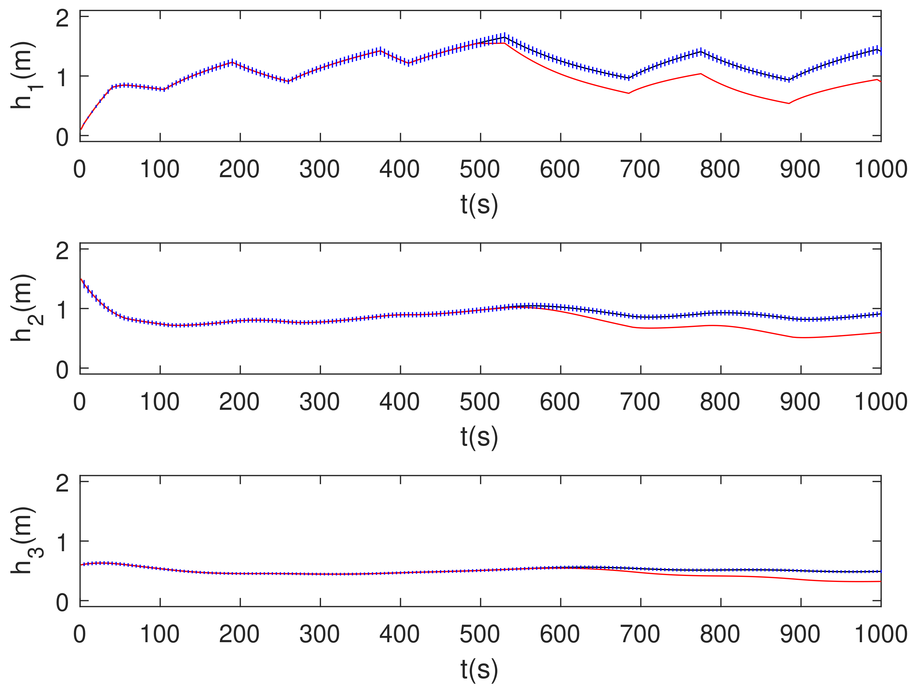
• The system is non-faulty until $t=500$ s, and from this time on, there is a leakage in tank 1 of approximately $0.25$% of the water inflow. The results are shown in Figure 6, where the bands are the results of the simulation using marks and the line is the values of the heights of the liquid in the tanks for the faulty system. The comparison shows the effect of the leakage. The line is below the band from the instant $t=500$ s for tank 1 and over the band for tanks 2 and 3.
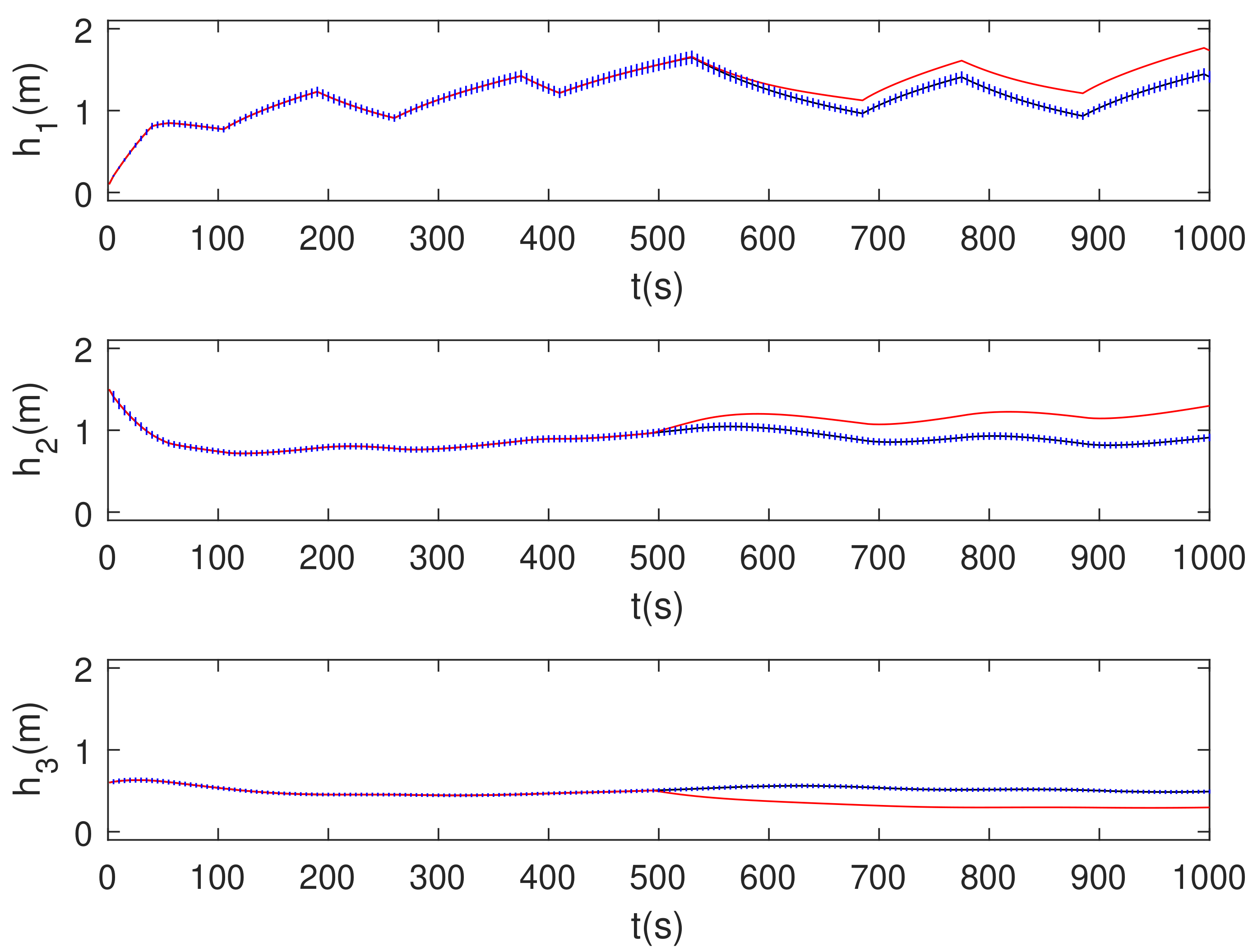
• The system is non-faulty until $t=500$ s and from this time on, there is a clogging between tanks 2 and 3 of 50% of the nominal flow. Figure 7 shows the effect of the clogging. The line is below the band from the instant $t=500$ s for tank 3 and over the band for tanks 2 and 1, some instants later.

The simulations were performed until $t=1000$ s to underline the comparisons.

3.4. Control

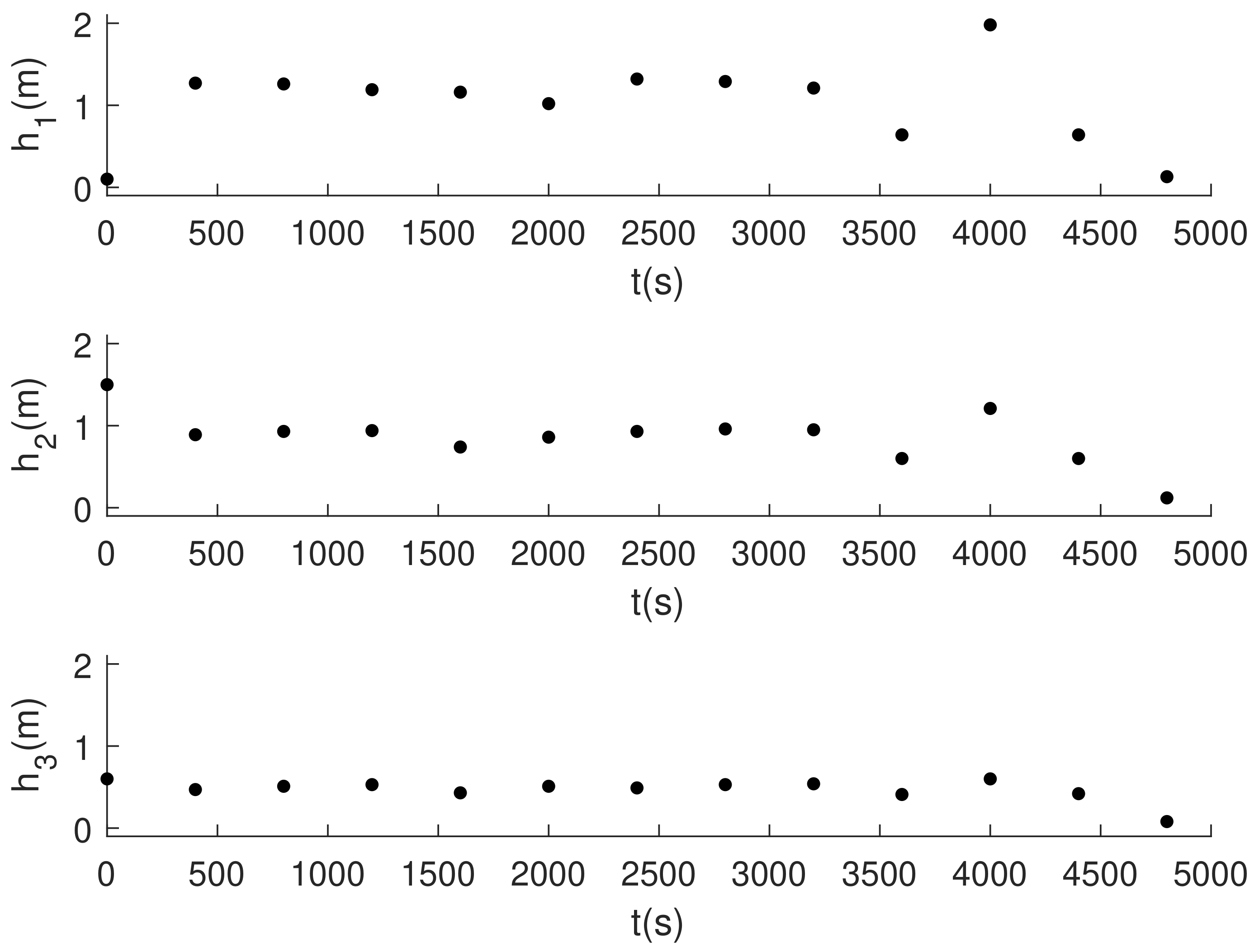
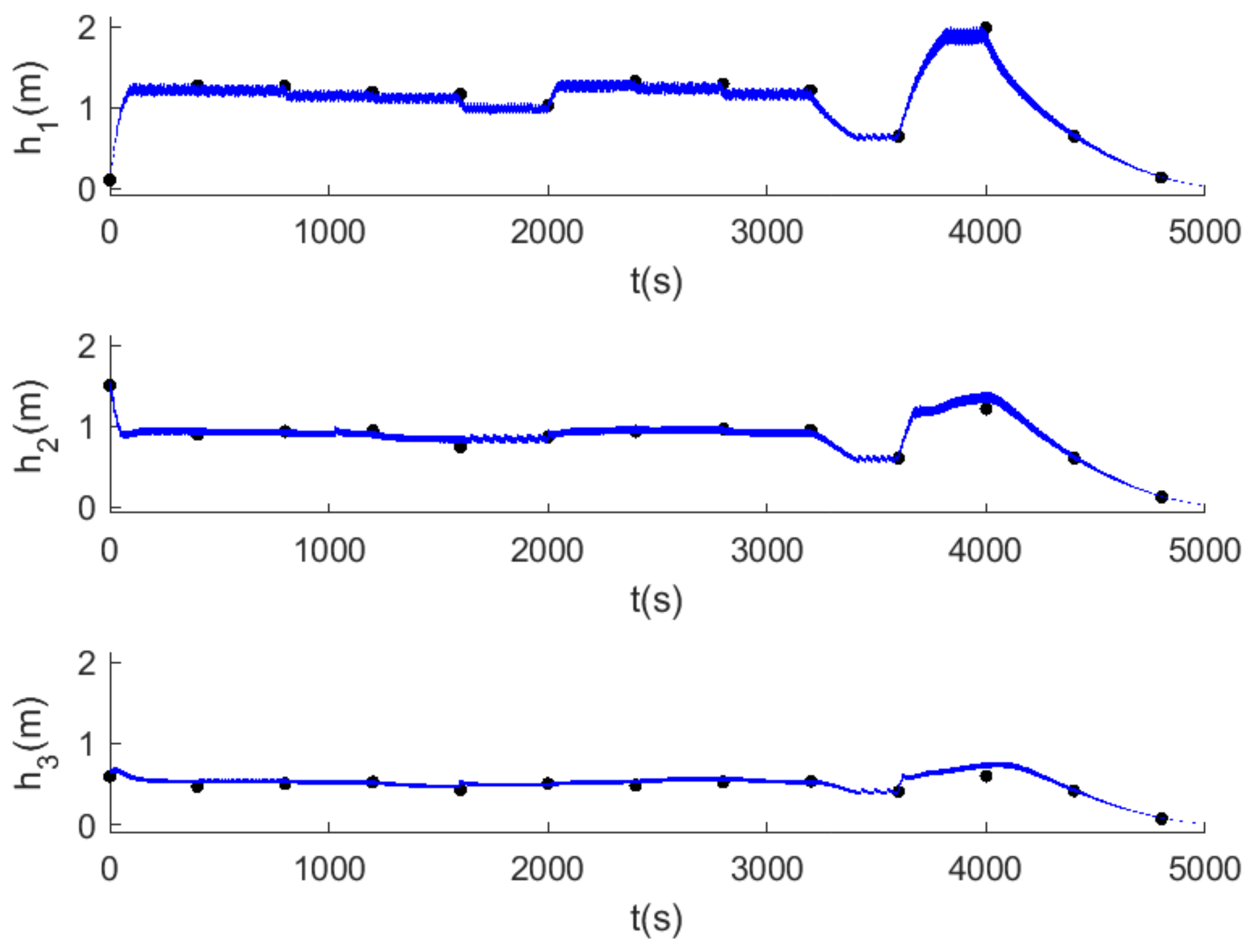
An elementary open-loop control was developed to show the usefulness of the model using marks in control systems. The process variables to be achieved are target heights of the liquid in the tanks, (or, in this test, arbitrarily chosen from the real simulation with the model, see Figure 2). For example, the ones represented by black dots in Figure 8. These outputs are controlled by the input flows to each tank in form of percentages $k_1\left(t\right),k_2\left(t\right),k_3\left(t\right)$ of the maximal flows $q_1=q_2=q_3=0.01$.

When at instant t, the later and nearest target height is above the interval associated to the output mark $h_1\left(t\right)$ or $h_2\left(t\right)$ or $h_3\left(t\right)$, then $k_1\left(t\right)=1$ or $k_2\left(t\right)=1$ or $k_3\left(t\right)=1$. When it is under, then $k_1\left(t\right)=0$ or $k_2\left(t\right)=0$ or $k_3\left(t\right)=0$. Finally, when it is inside the interval, then $k_1\left(t\right)=d_1\left(t\right)$ or $k_2\left(t\right)=d_2\left(t\right)$ or $k_3\left(t\right)=d_3\left(t\right)$, where $d_1\left(t\right)$ is the relative distance between the target height and the center of the interval $h_1\left(t\right)$ (the same for $d_2\left(t\right)$ and $d_3\left(t\right)$).

The result is a set of percentages for every instant, t. The output of the model is the band of associated intervals in Figure 9. The target heights are very close to being contained in the corresponding marks. Therefore, they can be considered consistent with the model for the inputs flows defined by $k_1\left(t\right)$, $k_2\left(t\right)$ and $k_3\left(t\right)$.

4. Conclusions

Real numbers are the “ideal” framework for dealing with quantities associated with physical phenomena. However, real numbers are not attainable and “disappear” when the observer obtains the value of a quantity. The alternative is digital numbers but a measurement value becomes a point on a digital scale depending on the phenomenon itself, the accuracy, correctness, and errors of the devices used in the measurement, and the numbers of digits used to represent it on the digital scale.

A mark represents, in a consistent procedure, the point information provided by a digital scale. The system of marks has an internal structure that reflects not only the losses of information inherent in the readings on a digital scale and the evolution of the computations from them, but also the indiscernibility of the observed phenomena.

The computations performed using marks also reflect the gradual loss of information, due to numerical errors and truncations, and give relevant warnings for decision making, either on the acceptability of the results or on the usefulness of seeking more precision to achieve the necessary validity.

In conclusion, marks are an appropriate framework for any iterative process, within current research conditions and certain assumptions, where uncertainty is significant and can be generalized when needed. For example, if the process is a long simulation with many steps or an iterative approach with slow convergence, it is necessary to control the accumulation of experimental, scaling, and computational errors so as not to let it exceed the tolerance set by the observer.

The benchmark presented is a good example of the use of marks for an iterative process. Marks prove to be a correct and satisfactory tool for modeling physical systems with uncertainties in their variables and parameters. Marks provide a double contribution to any computational process: (1) the granularity as a good timely test for the validity of any result, and (2) they provide meaning to any valid result by means of the semantic theorem. The final semantics of a simulation using marks is just the one needed for problems like fault detection, control, or parameter identification (via optimization) of a mathematical model against a set of experimental data with uncertainties. This opens a wide field of applications for marks.

References

- Kruse, R.; Schwecke, J.H. Uncertainty and Vagueness in Knowledge Based Systems Numerical Methods; Springer: Berlin/Heidelberg, Germany, 1991. [Google Scholar]
- Russel, B. Vagueness. Australas. J. Philos. 1923, 1, 84–92. [Google Scholar] [CrossRef]
- Black, M. Vagueness. Philos. Sci. 1937, 2, 427–455. [Google Scholar] [CrossRef]
- Moore, R.E. Interval Analysis; Prentice-Hall: Englewood Cliffs, NJ, USA, 1966. [Google Scholar]
- Moore, R.E. Methods and Applications of Interval Analysis; SIAM: Philadelphia, PA, USA, 1979. [Google Scholar]
- Gardenyes, E.; Mielgo, H.; Trepat, A. Modal intervals: Reasons and ground semantics. Lect. Notes Comput. Sci. 1986, 212, 27–35. [Google Scholar]
- Sainz, M.A.; Armengol, J.; Calm, R.; Herrero, P.; Jorba, L.; Vehi, J. Modal Interval Analysis: New Tools for Numerical Information; Springer: Berlin/Heidelberg, Germany, 2014; Volume 2091. [Google Scholar]
- Zadeh, L. Fuzzy sets. Inf. Control 1965, 8, 338–353. [Google Scholar] [CrossRef] [Green Version]
- Moore, R.; Lodwick, W. Interval analysis and fuzzy set theory. Fuzzy Sets Syst. 2003, 135, 5–9. [Google Scholar] [CrossRef]
- Pawlak, Z. Rough Set. Int. J. Comput. Inf. Sci. 1982, 11, 341–356. [Google Scholar] [CrossRef]
- Leibniz, G.W. Discourse on Metaphysics and the Monadology (Trans. George R. Montgomery); Prometeus Books (First Published by Open Court, 1902): New York, NY, USA, 1992. [Google Scholar]
- Valdes-Lopez, A.; Lopez-Bastida, E.; Leon-Gonzalez, J. Methodological approaches to deal with uncertainty in decision making processes. Univ. Soc. 2020, 12, 7–17. [Google Scholar]
- Xiao, H.; Cinnella, P. Quantification of model uncertainty in RANS simulations: A review. Prog. Aerosp. Sci. 2019, 108, 1–31. [Google Scholar] [CrossRef] [Green Version]
- Chen, S.M.; Zou, X.Y.; Gunawan, G.C. Fuzzy time series forecasting based on proportions of intervals and particle swarm optimization techniques. Inf. Sci. 2019, 500, 127–139. [Google Scholar] [CrossRef]
- Contreras, I.; Calm, R.; Sainz, M.A.; Herrero, P.; Vehi, J. Combining Grammatical Evolution with Modal Interval Analysis: An Application to Solve Problems with Uncertainty. Mathematics 2021, 9, 631. [Google Scholar] [CrossRef]
- Wang, L.; Liu, Y.; Liu, Y. An inverse method for distributed dynamic load identification of structures with interval uncertainties. Adv. Eng. Softw. 2019, 131, 77–89. [Google Scholar] [CrossRef]
- Lei, L.; Chen, W.; Xue, Y.; Liu, W. A comprehensive evaluation method for indoor air quality of buildings based on rough sets and a wavelet neural network. Build. Environ. 2019, 162, 106296. [Google Scholar] [CrossRef]
- Jorba, L. Intervals de Marques. Ph.D Thesis, Universitat de Barcelona, Barcelona, Spain, 2003. Available online: http://hdl.handle.net/2445/42085 (accessed on 31 August 2021).
- Sainz, M.A.; Calm, R.; Jorba, L.; Contreras, I.; Vehi, J. Marks: A New Interval Tool. GitHub Repository. 2021. Available online: https://github.com/MiceLab/MarksLibrary (accessed on 31 August 2021).
- Sainz, M.; Armengol, J.; Vehi, J. Fault detection and isolation of the three-tank system using the modal interval analysis. J. Process Control 2001, 12, 325–338. [Google Scholar] [CrossRef]
- Amira. Documentation of the Three Tank System; Amira GmbH: Duisburg, Germany, 1994. [Google Scholar]
Figure 1.
Schematic representation of the three-tank system.
Figure 2.
Three-tank system. Simulation results for the three state variables using real numbers.
Figure 3.
Three-tank system. Simulation results for the three state variables using real numbers. The dark bands are only apparent. They are the accumulation of the 1000 little vertical segments which represent the intervals associated to the resulting marks in the 1000 simulation points.
Figure 4.
Schematic representation of the extended three-tank system.
Figure 5.
Extended three-tank system. Simulation results for the three state variables using real numbers.The dark bands are only apparent. They are the accumulation of the 1000 little vertical segments which represent the intervals associated to the resulting marks in the 1000 simulation points.
Figure 6.
Faulty three-tank system: Leakage of approximately % of the water inflow in tank 1 from s. Blue bands represent the computation using marks while red lines correspond to the measured values of the three state variables.
Figure 7.
Faulty three-tank system: clogging between tanks 2 and 3 from s. Blue bands represent the computation using marks while red lines correspond to the measured values of the three state variables.
Figure 8.
Three-tank system. Target heights to be achieved in open loop control.
Figure 9.
Three-tank system. Simulation results for the open loop control of the liquid heights.
Publisher’s Note: MDPI stays neutral with regard to jurisdictional claims in published maps and institutional affiliations. |
© 2021 by the authors. Licensee MDPI, Basel, Switzerland. This article is an open access article distributed under the terms and conditions of the Creative Commons Attribution (CC BY) license (https://creativecommons.org/licenses/by/4.0/).
Share and Cite
MDPI and ACS Style
Sainz, M.A.; Calm, R.; Jorba, L.; Contreras, I.; Vehi, J. Marks: A New Interval Tool for Uncertainty, Vagueness and Indiscernibility. Mathematics 2021, 9, 2116. https://0-doi-org.brum.beds.ac.uk/10.3390/math9172116
AMA Style
Sainz MA, Calm R, Jorba L, Contreras I, Vehi J. Marks: A New Interval Tool for Uncertainty, Vagueness and Indiscernibility. Mathematics. 2021; 9(17):2116. https://0-doi-org.brum.beds.ac.uk/10.3390/math9172116
Chicago/Turabian StyleSainz, Miguel A., Remei Calm, Lambert Jorba, Ivan Contreras, and Josep Vehi. 2021. "Marks: A New Interval Tool for Uncertainty, Vagueness and Indiscernibility" Mathematics 9, no. 17: 2116. https://0-doi-org.brum.beds.ac.uk/10.3390/math9172116
Note that from the first issue of 2016, this journal uses article numbers instead of page numbers. See further details here.