Evaluation of Clustering Algorithms on HPC Platforms

Abstract

Clustering algorithms are one of the most widely used kernels to generate knowledge from large datasets. These algorithms group a set of data elements (i.e., images, points, patterns, etc.) into clusters to identify patterns or common features of a sample. However, these algorithms are very computationally expensive as they often involve the computation of expensive fitness functions that must be evaluated for all points in the dataset. This computational cost is even higher for fuzzy methods, where each data point may belong to more than one cluster. In this paper, we evaluate different parallelisation strategies on different heterogeneous platforms for fuzzy clustering algorithms typically used in the state-of-the-art such as the Fuzzy C-means (FCM), the Gustafson–Kessel FCM (GK-FCM) and the Fuzzy Minimals (FM). The experimental evaluation includes performance and energy trade-offs. Our results show that depending on the computational pattern of each algorithm, their mathematical foundation and the amount of data to be processed, each algorithm performs better on a different platform.

1. Introduction

Modern society generates an overwhelming amount of data from different sectors, such as industry, social media or personalised medicine, to name a few examples [1]. These raw datasets must be sanitised, processed and transformed to generate valuable knowledge in those contexts, which requires access to large computational facilities such as supercomputers. Current supercomputers are designed as heterogeneous systems, relying on Graphics Processing Units (GPUs), many-core CPUs and field-programmable gate arrays (FPGAs) to cope with this data deluge [2]. Heterogeneous computing architectures leverage several levels of parallelism, including instruction-level parallelism (ILP), thread-level parallelism (TLP) and data-level parallelism (DLP). This significantly complicates the efficient programming of such architectures. ILP and TLP have been traditionally exposed in latency-oriented and multicore architectures, but the best way to expose DLP is through vector operations. A vector design uses a single instruction to compute several data elements. Examples of vector designs include SIMD extensions [3,4,5,6,7], dedicated vector computing [8] and GPUs [9,10]. Therefore, the effective and efficient use of heterogeneous hardware remains a challenge.

Clustering algorithms are of particular interest when transforming data into knowledge. Clustering aims to group a set of data elements (i.e., measures, points, patterns, etc.) into clusters [11]. In order to determine these clusters, a similarity or distance metric is used. Common metrics used in these algorithms include Euclidean or Mahalanobis distance [12]. Individuals from a cluster are closer to its centre than to any other given cluster centre [13]. Clustering algorithms are critical to analyse datasets in many fields, including image processing [14], smart cities [15,16] or bioinformatics [17]. The most relevant clustering algorithms have the following characteristics: (1) scalability, i.e., theability to handle an increasing amount of objects and attributes; (2) stability to determine clusters of different shape or size; (3) autonomy or self-driven, i.e., it should require minimal knowledge of the problem domain (e.g., number of clusters, thresholds and stop criteria); (4) stability, as it must remain stable in the presence of noise and outliers; and, finally, (5) data independency to be independent of the way objects are organised in the dataset.

Several clustering algorithms have been proposed in the literature [18]. These algorithms perform an iterative process to find (sub)optimal solutions that tries to optimise a membership function (also known as clustering algorithms are NP-complex problems and their computational cost is very high when run on sufficiently large data sets) [19]. The computational cost of these algorithms is even higher for fuzzy clustering algorithms as they provide multiple and non-dichotomous cluster memberships, i.e., a data item belongs to different clusters with a certain probability. Several fuzzy clustering algorithms have been proposed in the literature. The fuzzy c-means (FCM) algorithm [20] was the first fuzzy clustering proposed. One of the main drawbacks of FCM is that requires to know the number of clusters to be generated in advance, like k-means. Then, the search space increases as the optimal number of clusters must be found, and therefore, the computational time increases. Another issue is that the FCM algorithm assumes that the clusters are spherical shaped. Several FCM-based algorithms have been proposed to detect different geometrical shapes in data sets. Among them, we may highlight the Gustafson and Kessel [21] algorithm which applies an adaptive distance norm to each cluster, also replacing the Euclidean norm in the by Mahalanobis distance. Finally, the Fuzzy Minimals (FM) clustering algorithm [22,23] does not need prior knowledge about the number of clusters. It also has the advantage that the clusters do not need to be compact and well separated. All these changes in the algorithm and/or scoring function imply an added computational cost that makes the parallelisation of these algorithms even more necessary in order to take advantage of all the levels of parallelism available in today’s heterogeneous architectures. In fact, several parallel implementations in heterogeneous systems have been proposed for some of these algorithms such as the FCM [24] and FM [25]. In this paper, different fuzzy clustering algorithms, running on different Nvidia and Intel architectures, are evaluated in order to identify (1) which is the best platform in terms of power and performance to run these algorithms and (2) what is the impact on performance and power consumption of the different features added in each of the fuzzy algorithms, so that the reader can determine which algorithm to use and on which platform, depending on their needs. The main contributions of this paper include the following.

• A description of the mathematical foundation of three fuzzy clustering algorithms.
• A detailed parallel implementation these clustering algorithms for different computing platforms.
• In-depth evaluation of HPC platforms and heavy workloads. Our results show the best evaluation platform for each algorithm.
• A performance and energy comparison is performed between different platforms, reporting performance improvements of up to 225×, 32× and 906× and energy savings of up 5.7×, 10× and 308× for FM, FCM and GK-FCM, respectively.

The rest of the article is organised as follows. Section 2 shows the related work before we analyse in detail the mathematical foundation for the selected clustering algorithms in Section 3. Then, Section 4 describes the CPU/GPU parallelisation and optimisation process. Section 5 shows performance and energy evaluation under different scenarios. Finally, Section 6 ends the paper with some conclusions and directions for future work.

2. Related Work

Clustering methods have been studied in great depth in the literature [26]. However, there are very few parallel implementations that cover different computing platforms. The k-means algorithm is one of the most studied clustering methods [27]. Hou [28], Zhao et al. [29] and Xiong [30] developed MapReduce solutions to improve k-means. Jin et al. proposed a distributed single-linkage hierarchical clustering algorithm (DiSC) based also on MapReduce [31]. The k-tree method is a hierarchical data structure and clustering algorithm to leverage clusters of computers to deal with extremely large datasets (tested on a 8 terabyte dataset) [32]. In [33], the authors optimise a triangle inequality k-means implementation using a hybrid implementation based on MPI and OpenMP on homogeneous computing clusters, however they do not target heterogeneous architectures.

Several papers have parallelised clustering algorithms on GPUs. For instance, Li et al. provide GPU parallelisation guidelines of the k-means algorithm. They describe data dimensionality as an important factor in terms of performance on GPUs [34]. Optimal tabu k-means clustering combines tabu search for calculation of centroids with clustering features of k-means [35]. Djenouri et al. proposed three single-scan (SS) algorithms that exploit heterogeneous hardware by scheduling independent jobs to workers in a cluster of nodes equipped with CPUs and GPUs [36]. In [37], the authors proposed a classifier for efficiently mining data streams which was based on machine learning improved by an efficient drift detector. However, they focused on hard clustering techniques where data elements only belong to one cluster and probabilities are not provided. Other works also proposed problem-specific parallelisation of the k-means algorithm. Image Segmentation [38], Circuit Transient Analysis [39], monitoring fault tolerance in Wireless Sensor Networks (WSN) [40], air pollution detection [15] and health care data classification [41] are examples of domain-specific k-means implementations.

Fuzzy clustering algorithms were introduced by Bezdek et al. [20] and they have as their main advantage that the membership function is not dichotomous; instead, each data item has a probability of belonging to each cluster. In other words, each data item can belong to more than one cluster. Furthermore, membership degrees can also express the degree of ambiguity with which a data item belongs to a cluster. The concept of degrees of membership is based on the definition of fuzzy sets [42]. Several parallelisation of fuzzy clustering algorithms have been proposed in the literature. For instance, Anderson et al. [43] introduced the first GPU implementation attempt of the FCM algorithm. They highlighted that one of the main bottlenecks was continuous reductions carried out to merge results from different clusters. Al-Ayyoub et al. [44] implemented a variant of the FCM (brFCM) on GPUs. They compared their implementation with a single-threaded CPU version by clustering lung CT and knee MRI images. Although their results offered 23.43× speed-up factor compared to the sequential version, this version did not exploit the multiple levels of parallelism available on the CPU such as vector units or multiple cores. Aaron et al. [45] demonstrated that the FCM clustering algorithm can be improved by the use of static and dynamic single-pass incremental FCM procedures. Although they did not provide a parallel version, they pointed out this is mandatory in the future work. Defour and Marin developed FuzzyGPU, a library for common operations for fuzzy arithmetics. More recently, Téllez-Velázquez, Arturo and Cruz-Barbosa [46] introduced an inference machine architecture that processes string-based rules and concurrently executes them based on an execution plan created by a fuzzy rule scheduler. This approach explored the parallel nature of rule sets, offering high speed-up ratios without losing generality. Cebrian et al. [47] first proposed coarse and fine grain parallelisation strategies in Intel and Nvidia architectures for the FM algorithm but it was not compared against other fuzzy algorithm. Finally. Scully-Alison et al. propose a sparse fuzzy k-means algorithm that operates on multiple GPUs [48] and performs clustering for real environmental sensor data.

3. Clustering Algorithms

Clustering algorithms are based on the assignment of data points to groups (also known as clusters). Points belonging to the same cluster can be considered to share a common similarity characteristic. This similarity is based on the evaluation (i.e., minimisation) of an objective function. This includes the use of different metrics, such as distance, connectivity and/or intensity. A different objective function can be chosen, depending on the characteristics of the dataset or the application.

As mentioned above, fuzzy clustering methods are a set of classification algorithms where each data point belongs to all clusters with a degree of probability of belonging. This probability could be 0, indicating that this point does not belong in any case to that set. In what follows, we show the mathematical foundations of the clustering algorithms targeted in this work, including the Fuzzy C-means (FCM), Gustafson–Kessel FCM (GK-FCM) and the Fuzzy Minimals (FM) algorithms [20,49,50]. These algorithms are well-known fuzzy clustering algorithms and they are commonly used in several applications [51].

In general terms, fuzzy clustering algorithms creates fuzzy partitions of the dataset.

Let us define $X=\left\{x_1,x_2,\dots ,x_n\right\}\subset {\mathbb{R}}^F,$ where F is the dimension of the vector space.

A fuzzy partition of X into c clusters $(1<c<n)$ is represented by a matrix $U=\left(u_{ij}\right)$ that satisfies

$$u_{ij}\in [0,1]\forall i,j;\sum _{i=1}^c{u}_{ij}=1\forall j;\sum _{j=1}^n{u}_{ij}>0\forall i.$$

$u_{ij}\in [0,1]$ represents the membership degree of datum $x_j$ to cluster i relative to all other clusters.

3.1. Fuzzy C-Means: FCM

FCM aims to find the fuzzy partition that minimises the objective function (1)

$$J_m(U,V)=\sum _{k=1}^n\sum _{i=1}^c{\left(u_{ik}\right)}^m{d}_{ik}^2,$$

(1)

where $V=\{v_1,v_2,\dots ,v_c\}$ are the centres of clusters, or prototypes, $d_{ik}$ is the distance function and m is a constant that represents the fuzziness value of the resulting clusters that are to be formed, $1\le m\le \infty$. The $u_{ij}$ is dependent on the distance function, $d_{ij}$. Bezdek proposed $m=2$, the Euclidean distance, $d_{ik}=\left|\right|x_j-v_k\left|\right|$, and

$$u_{ik}=\frac{1}{{\displaystyle \sum _{k=1}^c}{\left[\frac{d_{ij}}{d_{ik}}\right]}^{\frac{2}{m-1}}}$$

(2)

The calculation of the prototypes is performed by means of

$$v_i=\frac{{\displaystyle \sum _{k=1}^n}{\left(u_{ik}\right)}^m{x}_k}{{\displaystyle \sum _{k=1}^n}{\left(u_{ik}\right)}^m}.$$

(3)

FCM starts with a random initialisation of the membership values for each example of the manually selected clusters. The algorithm will iterate the clusters by recursively updating the cluster centres using the membership functions (2) and (3) until convergence criteria is reached. This is done in order to minimise the objective function (1). The convergence criteria is met when the overall difference in the membership function between the current and previous iteration is smaller than a given epsilon value, $ϵ$.

3.2. Gustafson–Kessel: GK-FCM

The Gustafson–Kessel (GK-FCM) is an evolution of the FCM algorithm [21]. It replaces the use of the Euclidean distance in the objective function by a cluster-specific Mahalanobis distance [52]. The goal of this replacement is to adapt to various sizes and forms of the clusters. For a given cluster j, the associated Mahalanobis distance can be defined as

$$d_{ij}^2={(x_i-v_j)}^t{\Lambda }_j^{-1}(x_i-v_j),$$

(4)

where

$${\Lambda }_j=\frac{{\displaystyle \sum _{k=1}^n}{\left(u_{ik}\right)}^m(x_i-v_j){(x_i-v_j)}^t}{{\displaystyle \sum _{k=1}^n}{\left(u_{ik}\right)}^m}\forall j=1,\dots ,c,$$

(5)

is the covariance matrix of the cluster.

Using the Euclidean distance in the objective function of FCM means, it is assumed that $\forall j,$$A_j=I$, identity matrix, i.e., all clusters have the same covariance that equals the identity matrix. Therefore, FCM can only detect spherical clusters, but it cannot identify clusters having different forms or sizes. Krishnapuram and Kim show that GK-FCM is better suited for ellipsoidal clusters of equal volume [53].

3.3. Fuzzy Minimals: FM

The FM algorithm, first introduced by Flores-Sintas et al. in 1998, provides scalability, adaptability, self-driven, stability and data independence to the clustering arena [22,23,50,54]. One useful feature of the FM algorithm is that it requires no prior knowledge of the number of prototypes to be identified in the dataset, as is the case with FCM and GK-FCM algorithms.

FM is a two-stage algorithm. In the first stage, the r factor for the input dataset is computed. The r factor is a parameter that measures the isotropy in the dataset. The calculation of r factor is shown in (6).

$$\frac{\sqrt{|C^{-1}|}}{n{r}^F}\sum _{x\in X}\frac{1}{1+r^2{d}_{x\overline{x}}^2}=1.$$

(6)

It is a nonlinear expression, where $|C^{-1}|$ is the determinant of the inverse of the covariance matrix, $\overline{x}$ is the mean of the sample X, $d_{x\overline{x}}$ is the Euclidean distance between x and $\overline{x}$, and n is the number of elements of the sample. The use of Euclidean distance implies that the homogeneity and isotropy of the features space are assumed. Whenever homogeneity and isotropy are broken, clusters are created in the features space.

Once the r factor is computed, the calculation of prototypes is executed to obtain the clustering result. The objective function used by FM is given by (7)

$$J_{\left(v\right)}=\sum _{x\in X}{\mu }_{xv}·d_{xv}^2,$$

(7)

where

$${\mu }_{xv}=\frac{1}{1+r^2·d_{xv}^2}.$$

(8)

Equation (8) is used to measure the degree of membership ofelement x to the cluster where v is the prototype. The FM algorithm performs an iterative process to minimise the objective function given by Equation (9), for the prototypes represented by each cluster. The input parameters ${\epsilon }_1$ and ${\epsilon }_2$ establish the error degree committed in the minimum estimation and show the difference between potential minimums, respectively.

$$v=\frac{{\sum }_{x\in X}{\mu }_{xv}^2·x}{{\sum }_{x\in X}{\mu }_{xv}^2}.$$

(9)

4. Parallelisation Strategies

4.1. Baseline Implementations

This section shows the different clustering methods pseudocodes. Functions for the baseline implementations are manually coded and parallelised using OpenMP. We do not show full codes due to space limitations. Note that ∘ represents a Hadamard product, ⊖ represents a Hadamard subtract and ⊘ represents a Hadamard division. These are product/subtraction/division of two matrices element by element. $A^{\overline{)n}}$ represents an element-wise exponent n for elements of matrix A. X is the input dataset to be classified in 2D matrix form, with size x rows and y columns. Notice that capital names refer to matrices while the rest of the variables refer to scalars.

4.1.1. FCM

Algorithm 1 shows the pseudocode for FCM. U represents the randomly chosen centres in 2D matrix form. $ex$ and $ix$ are precomputed values for the exponent with $m=2$ as described in Section 3.1. Lines 5 to 11 match the computation of the centres as described in Equation (3). Lines 12 to 14 match Equation (1) for $m=2$. Line 15 corresponds to Equation (2) for $m=2$. Lines 16 and 17 update the cluster centres.

Algorithm 1: Pseudocode for the main loop of the FCM algorithm.

1: $Load\_Dataset\left(X\right)$ 2: $Initialize\_Random\_Centers\left(U\right)$ 3: $ex\leftarrow 2/(2-1);ix\leftarrow -2/(2-1)$ 4: for$(step=0;step<iterations;step++)$do 5:   $U\_UP\leftarrow U^{\overline{)ex}}$ 6:   $SUM\_COLS\leftarrow ColumnWise\_Reduction(U\_U{P}^{⊺}:+)$ 7:    for $(i=0;i<y;i++)$ do 8:     ${\left[DC\right]}_i\leftarrow SUM\_COLS$ 9:    end for 10:   $NUMERATOR\leftarrow U\_UP\times X$ 11:   $CENTERS\leftarrow NUMERATOR\oslash D{C}^{⊺}$ 12:   $DISTANCE\_MATRIX\leftarrow Compute\_Euclidean\_Distance(CENTERS,X)$ 13:   $DM2\leftarrow DISTANCE\_MATRI{X}^{\overline{)2}}$ 14:   $OBJ\_FUNC\left[step\right]\leftarrow Reduction(DM2\circ U\_UP:+)$ 15:   $I\_DM2\leftarrow DISTANCE\_MATRI{X}^{\overline{)ix}}$ 16:   $SUM\_COL\_DIST\leftarrow ColumnWise\_Reduction(I\_DM2:+)$ 17:   $U\leftarrow ComputeRowWise(I\_DM2\oslash SUM\_COL\_DIST)$ 18:   $if\left(fabs\right(OBJ\_FUNC\left[step\right]-OBJ\_FUNC[step-1])<error)break;$ 19: end for

4.1.2. GK-FCM

Th GK-FCM algorithm is shown in Algorithm 2. As for the standard FCM, U represents the randomly chosen centres in 2D matrix form. $exponent$ and $inv\_exponent$ are precomputed values for the exponent with $m=2$ as described in Section 3.1. Lines 5 to 11 are identical to FCM and compute Equation (3). Lines 12 to 25 compute the Mahalanobis distance as described in Equations (4) and (5) for $m=2$. Line 26 corresponds to Equation (2) for $m=2$. Lines 27 and 28 update the cluster centres.

Algorithm 2: Pseudocode for the main loop of the GK-FCM algorithm.

1: $Load\_Dataset\left(X\right)$ 2: $Initialize\_Random\_Centers\left(U\right)$ 3: $ex\leftarrow 2/(2-1);ix\leftarrow -2/(2-1)$ 4: for$(step=0;step<iterations;step++)$do 5:   $U\_UP\leftarrow U^{\overline{)ex}}$ 6:   $SUM\_COLS\leftarrow ColumnWise\_Reduction(U\_U{P}^{⊺}:+)$ 7:   for $(i=0;i<y;i++)$ do 8:     ${\left[DC\right]}_i\leftarrow SUM\_COLS$ 9:    end for 10:   $NUMERATOR\leftarrow U\_UP\times X$ 11:   $CENTERS\leftarrow NUMERATOR\oslash D{C}^{⊺}$ 12:   for $(cluster=0;cluster<clusters;cluster++)$ do 13:   for (i = 0; i < x; i++) do 14:      ${\left[ZV\right]}_i\leftarrow {\left[X\right]}_i\ominus {\left[CENTERS\right]}_{cluster}$ 15:   end for 16:    $TMP\leftarrow {\left[Z{V}^{⊺}\right]}_i\circ {[U\_U{P}^{⊺}]}_{cluster}$ 17:    $COV\_MATRIX\leftarrow TMP\times ZV$ 18:    $COV\_MATRIX\leftarrow COV\_MATRIX\oslash SUM\_COLS\left[cluster\right]$ 19:    $det\leftarrow Compute\_Determinant(COV\_MATRIX)$ 20:    $power\_det\leftarrow de{t}^{(1/columns)}$ 21:    $MAHALANOBIS\leftarrow COV\_MATRI{X}^{-1}\circ power\_det$ 22:    $TMP\_DIST\leftarrow ZV\times MAHALANOBIS$ 23:    $TMP\_DIST\leftarrow TMP\_DIST\circ ZV$ 24:    $DIST\left[cluster\right]\leftarrow Row\_Reduction(TMP\_DIST:+)$ 25:  end for 26:   $I\_DM2\leftarrow DIS{T}^{\overline{)ix}}$ 27:   $SUM\_COL\_DIST\leftarrow ColumnWise\_Reduction(I\_DM2:+)$ 28:   $U\leftarrow ComputeRowWise(I\_DM2\oslash SUM\_COL\_DIST)$ 29:   $if\left(fabs\right(OBJ\_FUNC\left[step\right]-OBJ\_FUNC[step-1])<error)break;$ 30: end for

4.1.3. FM

Finally, Algorithm 3 depicts the main building blocks of FM algorithm. FM is composed of two main parts: (1) the calculation of the r factor (line 4, see Algorithm 4) and (2) the calculation of prototypes or centroids (lines 5 to complete the set V).

Algorithm 3: Pseudocode for the FM algorithm, V is the algorithm output that contains the prototypes found by the clustering process. F is the dimension of the vector space.

1: Choose ${\epsilon }_1$ and ${\epsilon }_2$ standard parameters. 2: Initialise $V=\left\{\right\}\subset {\mathbb{R}}^F$. 3: $Load\_Dataset\left(X\right)$ 4: $r\leftarrow Calculate\_r\_Factor\left(X\right)$ 5: $Calculate\_Prototypes(X,r,{\epsilon }_1,{\epsilon }_2,V)$

Algorithm 4: Pseudocode for the $Calculate\_r\_Factor$ of the FM algorithm.

1: $r\leftarrow 1$ 2: $e\leftarrow 0$ 3: for$(i=0;i<rows;i++)$do 4:   $det\leftarrow Compute\_Determinant(Covariance\_Matrix(X,rows\left)\right)$ 5:   $f1\leftarrow f1+(1/SRQT(det\left)\right)$ 6: end for 7: $comp\leftarrow abs(r-e)$ 8: while ($(comp>error)AND(cont<rows\times columns)$) do 9:    $cont++$ 10:   $e1\leftarrow r$ 11:   $f2\leftarrow 0$ 12:   for ($i=0;i<rows;i++$) do 13:    $tmp\leftarrow 0$ 14:    for ($k=0;k<columns;k++$) do 15:     $tmp\leftarrow tmp+{(X[i\times columns+k]-median\left[k\right])}^2$ 16:   end for 17:    $f2\leftarrow f2+(1/(1+r\times r\times tmp)$ 18:  end for 19:   $r\leftarrow {((f1\times f2)/rows)}^{1/columns}$ 20:  if $r>e$ then 21:    $comp\leftarrow r-e$ 22:  else 23:    $comp\leftarrow e-r$ 24:  end if 25: end while

The pseudocode for the $Calculate\_Prototypes$ function is quite large, so instead we will show the formulation for each function step (Algorithm 5).

Algorithm 5:$Calculate\_Prototypes\left(\right)$ of FM algorithm.

1: for$k=1;k<n;k=k+1$do 2:  $v_{\left(0\right)}\leftarrow x_k$, $t\leftarrow 0$, $E_{\left(0\right)}\leftarrow 1$ 3:  while $E_{\left(t\right)}\ge {\epsilon }_1$ do 4:    $t\leftarrow t+1$ 5:   ${\mu }_{xv}\leftarrow \frac{1}{1+r^2·d_{xv}^2}$, using $v_{\left(t-1\right)}$ 6:    $v_{\left(t\right)}\leftarrow$$\frac{{\sum }_{x\in X}{\left({\mu }_{xv}^{\left(t\right)}\right)}^2·x}{{\left({\mu }_{xv}^{\left(t\right)}\right)}^2}$ 7:    $E_{\left(t\right)}\leftarrow {\sum }_{\alpha \leftarrow 1}^F\left(v_{\left(t\right)}^{\alpha }-v_{\left(t-1\right)}^{\alpha }\right)$ 8:  end while 9:  if ${\sum }_{\alpha }^F\left(v^{\alpha }-w^{\alpha }\right)>{\epsilon }_2$, $\forall w\in V$ then 10:   $V\equiv V+\left\{v\right\}$. 11:  end if 12: end for

4.2. CPU Optimisations

CPU-based optimisations require all levels of parallelism (instruction, thread and data). Instruction-level parallelism is developed by the compiler, and we focus our programming efforts on thread and data-level parallelism. Our code is implemented using OpenMP, exploiting thread-level parallelism. However, its performance is sub-optimal, as we do not use well-known techniques to optimise matrix operations such as blocking/tiling. The code needs to be vectorised to fully exploit SIMD units and thus leverage data-level parallelism. Instead of doing this manually, we will rely on the Eigen library whenever possible [55]. Eigen will parallelise, vectorise and perform other optimisations, such as blocking/tiling, transparently.

Algorithm 6: Eigen pseudocode for the main loop of the FCM algorithm.

1: $Load\_Dataset\left(X\right)$ 2: $Initialize\_Random\_Centers\left(U\right)$ 3: $ex\leftarrow 2/(2-1);ix\leftarrow -2/(2-1)$ 4: for$(step=0;step<iterations;step++)$do 5:   $U\_UP\leftarrow U^{\overline{)ex}}$ 6:   $U\_UP\_T\leftarrow U\_UP.transpose\left(\right)$ 7:   $SUM\_COLS\leftarrow U\_UP\_T.rowwise\left(\right).sum\left(\right)$ 8:   $DC.colwise\left(\right)\leftarrow SUM\_COLS$ 9:    $DC\_T\leftarrow DC.transpose\left(\right)$ 10:   $NUMERATOR\leftarrow U\_UP\times X$ 11:   $CENTERS\leftarrow NUMERATOR.array\left(\right)/DC\_T.array\left(\right)$ 12:   $DISTANCE\_MATRIX\leftarrow Compute\_Euclidean\_Distance(CENTERS,X)$ 13:   $DM2\leftarrow DISTANCE\_MATRI{X}^{\overline{)2}}$ 14:   $OBJ\_FUNC\left[step\right]\leftarrow \left(\right(DM2.array\left(\right)\times U\_UP.array\left(\right)).sum()$ 15:   $I\_DM2\leftarrow DISTANCE\_MATRI{X}^{\overline{)ix}}$ 16:   $SUM\_COL\_DIST\leftarrow I\_DM2.rowwise\left(\right).sum\left(\right)$ 17:   $U\leftarrow I\_DM2.array\left(\right).rowwise\left(\right)/SUM\_COL\_DIST.array\left(\right))$ 18:   $if\left(fabs\right(OBJ\_FUNC\left[step\right]-OBJ\_FUNC[step-1])<error)break;$ 19: end for

Algorithm 6 shows the pseudocode for FCM using Eigen calls. Note that Lines 5, 12, 13 and 15 remain as function calls to our original code. We could not find an optimal way to implement them using Eigen.

Algorithm 7: Eigen pseudocode for the main loop of the GK-FCM algorithm.

1: $Load\_Dataset\left(X\right)$ 2: $Initialize\_Random\_Centers\left(U\right)$ 3: $ex\leftarrow 2/(2-1);ix\leftarrow -2/(2-1)$ 4: for$(step=0;step<iterations;step++)$do 5:   $U\_UP\_T\leftarrow U\_UP.transpose\left(\right)$ 6:   $SUM\_COLS\leftarrow U\_UP\_T.rowwise\left(\right).sum\left(\right)$ 7:   $DC.colwise\left(\right)\leftarrow SUM\_COLS$ 8:   $DC\_T\leftarrow DC.transpose\left(\right)$ 9:   $NUMERATOR\leftarrow U\_UP\times X$ 10:   $CENTERS\leftarrow NUMERATOR.array\left(\right)/DC\_T.array\left(\right)$ 11:   $U\_UP\leftarrow U^{\overline{)ex}}$ 12:  for $(cluster=0;cluster<clusters;cluster++)$ do 13:    $ZV\leftarrow X.array\left(\right).rowwise\left(\right)-CENTERS.row\left(cluster\right).array\left(\right)$ 14:    $ZV\_T\leftarrow ZV.transpose\left(\right)$ 15:    $TMP\leftarrow ZV\_T.array\left(\right).rowwise\left(\right)\times U\_UP\_T.row\left(cluster\right).array\left(\right)$ 16:    $COV\_MATRIX\leftarrow TMP\times ZV$ 17:    $COV\_MATRIX\leftarrow COV\_MATRIX.array\left(\right)/SUM\_COLS\left(cluster\right)$ 18:    $det\leftarrow COV\_MATRIX.determinant\left(\right)$ 19:    $power\_det\leftarrow de{t}^{(1/columns)}$ 20:    $COV\_MATRIX\_I\leftarrow COV\_MATRIX.inverse\left(\right)$ 21:    $MAHALANOBIS=COV\_MATRIX\_I\circ power\_det$ 22:    $TMP\_DIST\leftarrow ZV\times MAHALANOBIS$ 23:    $TMP\_DIST\leftarrow ZV.array\left(\right)\times TMP\_DIST.array\left(\right)$ 24:    $DIST\left[cluster\right]\leftarrow TMP\_DIST.colwise\left(\right).sum\left(\right)$ 25:  end for 26:   $I\_DM2\leftarrow DIS{T}^{\overline{)ix}}$ 27:   $SUM\_COL\_DIST\leftarrow I\_DM2.rowwise\left(\right).sum\left(\right)$ 28:   $U\leftarrow I\_DM2.array\left(\right).rowwise\left(\right)/SUM\_COL\_DIST.array\left(\right))$ 29:   $if\left(fabs\right(OBJ\_FUNC\left[step\right]-OBJ\_FUNC[step-1])<error)break;$ 30: end for

Algorithm 7 shows the pseudocode for GK-FCM using Eigen calls. As in FCM, there are several function calls that remain as in the original code. This includes lines 5, 21 and 26. Again, we could not find an optimal way to implement them using Eigen.

Finally, the FM algorithm performance carving is shown. First of all, a profiling analysis of the $Calculate\_r\_Factor$ is provided, revealing that the convolution and determinant steps are the most time consuming. This function is parallelised through OpenMP and Eigen library. This function shows a very good scalability, almost linear with thread count, as there are almost no critical sections in the code, just a final reduction to merge all partial factor r computations.

For the $Calculate\_Prototypes$ function, it can be parallelised using OpenMP (see Algorithm 5) as well. This parallelisation is not straight-forward as it requires a critical section (lines 9 and 10) to include candidate prototypes into the final output. The number of critical access to this memory is $O\left(N\right)$, where N is the number of prototypes found in the solution. As this number is unknown, a dynamic array must be developed, so as many prototypes found, as longer will take the execution. Fine-grain parallelisation via manual vectorisation is performed in lines 6–7 and the Euclidean distance required in line 5, being the later the most time consuming (around 90% of total execution time). A pseudocode of the SIMD version of the euclidean distance is shown in Algorithm 8. However, there are several limitations to this code: (a) horizontal operations (reduction), (b) increased L2 cache misses with high number of dimensions (columns), (c) low arithmetic intensity (A measure of operations performed relative to the amount of memory accesses (Bytes).) and (d) the division in Algorithm 5 line 5.

Algorithm 8: SIMD version of Algorithm 5 line 5.

1: for$l=0;l<columns;l+=SIMD\_WIDTH$do 2:   $aux\leftarrow simd\_load\left(PROTOTYPE\right[l\left]\right)-simd\_load\left(ROW\right[l\left]\right)$ 3:   $distance\leftarrow distance+aux\times aux$ 4: end for 5: $scalar\_distance\leftarrow reduce\_add\left(distance\right)$ 6: $output\leftarrow \frac{1}{1+rFactorSquare\times scalar\_distance}$

To solve some of these issues, we performed manual unrolling of the main loop to make use of the SIMD divisor ports available in the system. The unroll factor will be 16 iterations (rows) of the main loop (see Algorithm 5). All distances are then calculated by combining them into two vector registers. These registers can be then passed to the vector units (Algorithm 9. We rely on AVX-512 for this implementation. Other unrolling factors yield slightly worse performance results. This version puts more pressure on the memory subsystem, but the use of the SIMD division ports improves overall performance.

Algorithm 9: Superblocked SIMD version of Algorithm 5 line 5 (16 iterations) for a vector register of 8 doubles (512-bits).

1: for$bloc{k}_{c}ount=0;bloc{k}_{c}ount<16;bloc{k}_{c}ount++$do 2:   $aux\leftarrow 0;distance\left[bloc{k}_{c}ount\right]\leftarrow 0$ 3:   for $l=0;l<columns;l+=SIMD\_WIDTH$ do 4:     $aux\leftarrow simd\_load\left(PROTOTYPE\left[l\right]\right)-simd\_load\left(ROW[l+bloc{k}_{c}ount*columns]\right)$ 5:     $distance\left[bloc{k}_{c}ount\right]\leftarrow distance\left[bloc{k}_{c}ount\right]+aux\times aux$ 6:   end for 7:    $scalar\_distance\left[bloc{k}_{c}ount\right]\leftarrow reduce\_add\left(distance\left[bloc{k}_{c}ount\right]\right)$ 8: end for 9: $simd\_output1\leftarrow \frac{[1..1]}{[1..1]+[rFactorSquare..rFactorSquare]\times scalar\_distance[0..7]}$ 10: $simd\_output2\leftarrow \frac{[1..1]}{[1..1]+[rFactorSquare..rFactorSquare]\times scalar\_distance[8..15]}$

4.3. GPU Optimisations

This section shows the different parallelisation strategies developed with CUDA programming language for the three algorithms described in Section 4. These parallelisation approaches use a set of techniques and libraries to optimise their performance: (1) shared memory to optimise device memory accesses at block level and (2) cuBLAS to provide optimised functions to perform matrix operations and factorisations.

Algorithm 10 shows the FCM pseudocode. It shows the kernel and library function calls. This algorithm comprises a number of steps. The first four lines load the input data into the CPU and later on GPU. In addition, the $fuzzy\_U$ matrix is generated on the GPU using curand library. Next, lines 6 to 10 calculate the centre matrix ($centers$). Previously, three kernels and a call to cuBLAS calculate preliminary results. Lines 6 to 8 calculate the numerator ($numerator\_m$) of Equation (9) and line 9 calculates the denominator ($denominator\_m$). Then, the distance between the data matrix (X) and the centre matrix ($center$) is calculated in line 10. With this new distance matrix ($distance$), the error is calculated with a reduction ($reduce$) (see line 10). This error is tested to continue with the next iteration or end the execution.

Algorithm 10:FCM algorithm in GPU.

1: $Load\_Dataset\left(X\right)$ 2: $EXP=2/(2-1);inv\_exponent=-2/(2-1)$ 3: $init\_random\_centers\left(states\right);$ 4: $init\_u(states,fuzzy\_u);$ 5: for$step=1;i<MAX\_STEPS;i=i+1$do 6:   $exponent<<<bk,th>>>(fuzzy\_based\_u,fuzzy\_u,EXP);$ 7:   $cuBLASDGEMM(vector\_u\_columns,fuzzy\_base{d}_u);$ 8:   $numerator\_i<<<bk,th>>>(numerator\_m,fuzzy\_base{d}_u,vector\_u\_columns);$ 9:   $determinator\_i<<<bk,th>>>(denominator\_m,vector\_u\_columns);$ 10:   $centers\_i<<<bk,th>>>(center,numerator\_m,denominator\_m);$ 11:   $distance\_matrix\_i<<<bk,th>>>(distance,center,X);$ 12:   $Error\_i=reduce<<<bk,th>>>\left(distance\right);$ 13:   if $(Error\_ste{p}_i-Error\_ste{p}_{i-1})<error$ then 14:    $break;$ 15:   end if 16:   $new\_fuzzy\_u<<<bk,th>>>(fuzzy\_u,distance);$ 17: end for 18: $cudaMemcpy(u\_host,fuzzy\_u);$

Algorithm 11 shows the pseudocode for the Gustafson–Kessel Algorithm (GK-FCM), highlighting again kernel and library calls. This algorithm has a different set of computational and operational characteristics than the FCM algorithm. The FCM-GK algorithm performs a pre-normalisation of the data. It also contains operations such as the calculation of the inverse and transpose of a matrix in the calculation of different clusters. The computation of the inverse matrix is performed by using the cublasDgetriBatched function and for the computation of the transpose the kernel called ($traspose$).

As in the FCM algorithm, the algorithm can be divided into several steps. In the first five lines, the input matrix is normalised and then several data structures are initialised on the GPU. Next (lines 7–12), the ($center$) matrix is calculated, similar to Algorithm 10. The main difference in the process of both algorithms occurs from lines 13 to 24 where the ($distance$) matrix is calculated. The process consists of obtaining a matrix called ($covariance\_matrix$) and calculating its determinant and inverse. To perform this process, a set of functions from the cuBLAS library is used to achieve: (1) the LU factorisation and calculate the determinant and (2) we obtain the inverse of the matrix. The process is repeated as long as the result is not lower than the proposed error (lines 25–28).

Algorithm 11:FCM-GK algorithm in GPU.

1: $Load\_Dataset\left(X\right)$ 2: $EXP=2/(2-1);inv\_exponent=-2/(2-1)$ 3: $init\_random\_centers\left(states\right);$ 4: $init\_normalize\_data\left(X\right);$ 5: $init\_u(states,fuzzy\_u);$ 6: for$step=1;i<MAX\_STEPS;i=i+1$do 7:   $exponent<<<bk,th>>>(fuzzy\_exponent\_u,fuzzy\_u,EXP);$ 8:   $transpose<<<bk,th>>>(traspose\_u,fuzzy\_u);$ 9:   $cuBLASDGEMM(vector\_u\_columns,fuzzy\_exponent\_u);$ 10:   $numerator<<<bk,th>>>(numerator\_m,fuzzy\_exponent\_u,vector\_u\_columns);$ 11:   $determinator<<<bk,th>>>(denominator\_m,vector\_u\_columns);$ 12:   $centers<<<bk,th>>>(center,numerator\_m,denominator\_m);$ 13:   for $cluster=1;cluster<clusters;cluster=cluster+1$ do 14:    $substraction<<<bk,th>>>(ZV,X,center);$ 15:    $transpose<<<bk,th>>>(Z{V}_t,ZV);$ 16:    $cuBLASDGEMM(ZV\_temp,ZV\_t,fuzzy\_exponen{t}_u,vector\_u\_columns);$ 17:    $Covarianze\_matrix<<<bk,th>>>(Covarianze,ZV\_temp,ZV\_t,fuzzy\_exponent\_u);$ 18:    $Calculation\_cuBLASDGETRF\left(Covarianze\right);$ 19:    $determinant\_value=thrust::reduce(Covarianze\_factorized);$ 20:    $cuBLASDGETRI(Inverse\_matrix,Covarianze);$ 21:    $exponent<<<bk,th>>>(MAHALANOBIS\_matrix,Inverse\_matrix,determinant\_value);$ 22:    $cuBLASDGEMM(distance\_temp,ZV,MAHALANOBIS\_matrix);$ 23:    $reduction<<<bk,th>>>(distance,distance\_tmp,cluster);$ 24:  end for 25:   $new\_fuzzy\_u<<<bk,th>>>(fuzzy\_u,distance);$ 26:   if $(Error\_ste{p}_i-Error\_ste{p}_{(}i-1))<error$ then 27:    $break;$ 28:  end if 29: end for 30: $cudaMemcpy(u\_host,fuzzy\_u);$

As previously mentioned, the FM algorithm is divided into two stages. The first stage is the calculation of the r factor that is used in the second stage, called prototype calculation. In this case, the data are grouped together based on their distance. The parallelisation of both stages in GPU is briefly explained in Algorithm 12. First, the so-called r factor (lines 2–6) is calculated. For one of the rows of the data matrix (X), the covariance matrix is built and factored through Nvidia cuBLAS library. The diagonal of its factorisation is reduced to obtain the value of the determinant. Then, the calculation shown in line 5 is applied to each of the values and carries over to the previous ones to eventually obtain the r factor. The second step of the FM algorithm is the calculation of prototypes. In the first stage of this calculation, a set of candidate prototypes is calculated with the probability of belonging to each prototype (lines 9–14). This process consists of four kernels where each row of the data matrix (X) approaches a possible prototype. This calculation reproduces Equation (8). With these data obtained in this first stage, prototypes are included in the final set based on the distance between the prototypes included in the final set and each of the candidates. Finally, it is important to note that the number of columns in the data matrix (X) is a relevant factor for all clustering algorithms discussed in terms of performance on GPU platforms.

Algorithm 12:R Factor and Prototype calculation algorithm in GPU.

1: $Load\_Dataset\left(X\right)$ 2: for$i=0;i<rows;i=i+1$do 3:   $covariance\_matrix<<<bk,th,sh>>>(X,row\_i,rows,cols);$ 4:   $detvalue=cuBLAS\_reduction\left(covarianz{e}_{m}atrix\right);$ 5:   $rfactor+=\frac{1}{\sqrt{detvalue}};$ 6: end for 7: for$i=0;i<rows;i=i+1$do 8:   $cudaMemcpy(prot\_actual,X+i);$ 9:  while $erro{r}_i<erro{r}_1$do 10:    $new\_prot<<<bk,th>>>(X,rfactor,i,MU\_prot));$ 11:    $reduction<<<bk,th>>>(MU\_all,MU\_prot);$ 12:    $distance\_prots<<<bk,th>>>(distance,new\_prot,prot\_actual,MU\_all);$ 13:    $reduction<<<bk,th>>>(erro{r}_i,distance);$ 14:  end while 15:   $cudaMemcpy(provisional\_prototype+i,prot\_actual);$ 16: end for 17: for$i=0;i<rows;i=i+1$do 18:   $distance\_prots<<<bk,th>>>(prots\_d,provisional\_prototype+i,erro{r}_2);$ 19: end for 20: $cudaMemcpy(prots,prots\_d);$

5. Evaluation

This section introduces the performance and energy evaluation for all fuzzy clustering algorithms targeted and parallelisation approach proposed on different heterogeneous systems based on Intel CPUs and Nvidia GPUs.

5.1. Hardware Environment and Benchmarking

Intel-based platform 

We use an Intel Skylake-X i7-7820X CPU processor (SKL in our Figures). It has eight physical cores with sixteen threads running at 3.60 GHz (but we disabled simultaneous multi-threading, so we only have 8 threads available). It has 32 + 32 KB of L1 and 1MB of L2 cache per core plus 11MB of shared L3 cache. We chose this CPU as it is the only one available to us with support for AVX-512 (512-bit registers) instructions.

Nvidia-based platform 

Two GPU-based platforms are targeted. One node with a x86-based architecture and a Nvidia A100 GPU. This GPU belongs to Ampere family and it has 6912 CUDA cores at up to 1.41 GHz with FP32 compute performance of up to 19.5 TFLOPS, and 40 GB of 2.4 GHz HBM2 memory with 1.6 TB of bandwidth. The another node is an IBM POWER 9 system with two 16-core Power 9 processors at 2.7 GHz including an Nvidia V100 GPU with 5120 CUDA cores and 32 HBM2 memory with 870 GBps of bandwidth.

To test our parallelisation approaches, a dataset based on 800 K points that belongs to three hyper-ellipsoids is proposed. They are $S_k$, with $S_k\subset {\mathbb{R}}^{108}$, $\forall k\in \{1,2,3\}$, and $S_i\cap S_j=\forall i\ne j$. The cardinal of each subset is $|S_1|=\mathrm{271,060}$, $|S_2|=\mathrm{277,256}$ and $|S_3|=\mathrm{251,684}$, respectively.

5.2. Runtime Evaluation

Performance and energy figures are provided by varying the number of rows and columns of the input dataset. Columns represent the number of variables for each element in the dataset (e.g., for a dataset composed of bicycles, each column represents a characteristic, like brand, colour, type, etc.). Rows represent different data instances to be clustered (e.g., different data points). Our goal is to show the scalability on each dimension, as each field of application has different requirements. The parallel CPU version runs on 8 threads with AVX-512 support for all algorithms.

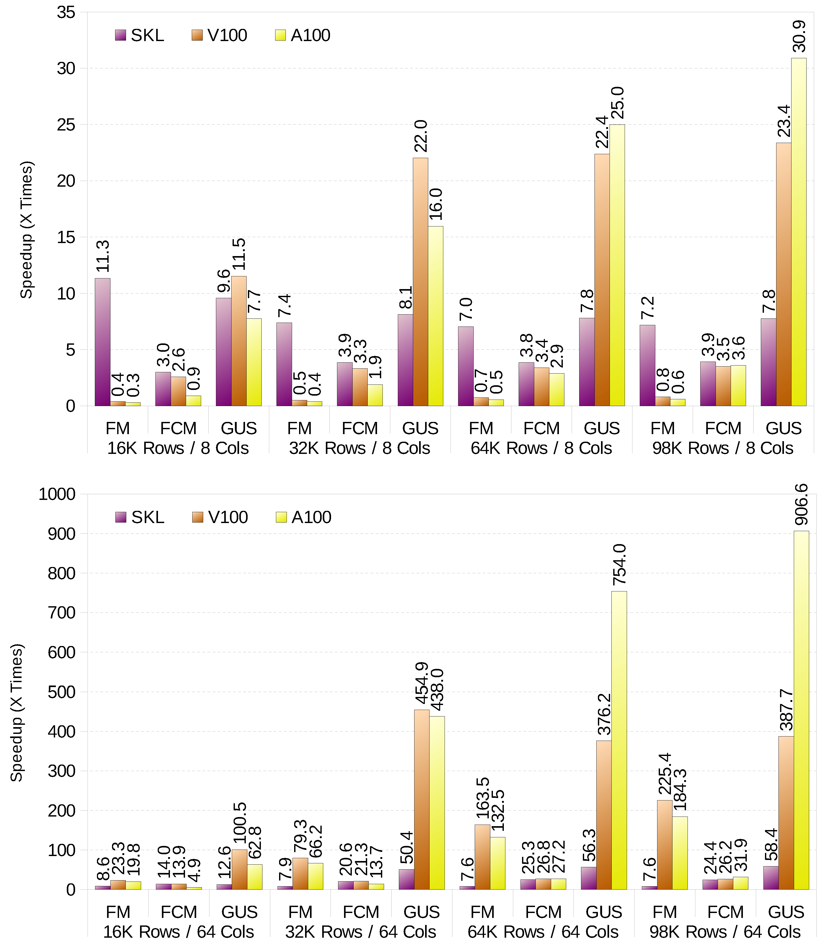
Figure 1 shows the performance gains compared to the baseline implementation, described in Section 4.1, for each clustering method. It shows results for 8 variables/columns (top) and 64 variables (bottom). It is important to note that the baseline implementation does not make use of SIMD units and only runs on a single thread. For small datasets with a small number of variables (up to 16 columns), the CPU outperforms the GPU for both FM and FCM. The CPU is specially good for FM with small datasets. However, as the computation of the r factor time increases with the dataset size, the additional computing power of the GPU starts to pay off. Nevertheless, the CPU always defeats the GPU when it calculates the prototypes, so a hybrid CPU-GPU implementation would be the best option. The differences in performance for high variable count in FCM are minimal, and go in favour of the GPU. On the other hand, GK-FCM (GUS in the Figure 1) always works best on the GPU. The reason is that the CPU is underutilised (less than 1% usage), as it spends most of the time in data movements (e.g., transpose). The analysed GPUs seem to be specially good at performing this task, and thus overwhelming performance improvements shown in the figure.

5.3. Energy Evaluation

This section shows an energy evaluation of the different clustering algorithms. We compare the energy measurements of the CPU package, that is, Intel’s performance counter that measures the energy consumed by the whole processor via the RAPL interface and the energy used by the whole GPU board. It is important to note that the GPU also requires CPU computations, but as the CPUs used in GPU clusters are usually over provisioned, we decided to compare strictly CPU vs. GPU energy.

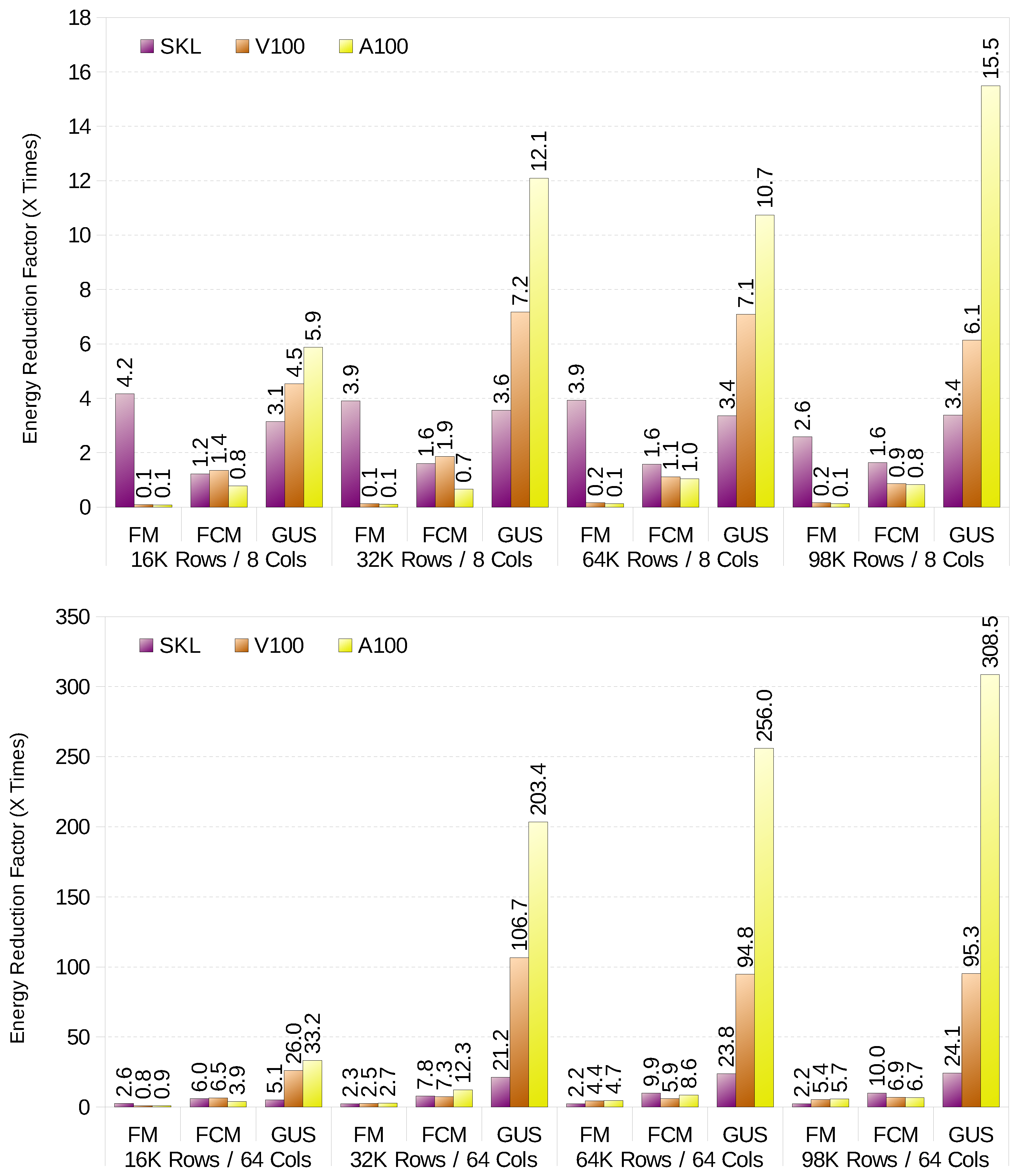
Figure 2 shows the energy reduction factor, that is, how many times the energy is reduced compared to the scalar implementation running on one CPU thread. When energy is taken into consideration, the differences between the CPU and GPU implementations of FM drop drastically. For example, with big datasets with high variable count, the CPU only uses 2.6× more energy than the GPU, while the performance is 29.6× faster in favour of the GPU. Still, it is a better option to run FM on the GPU for big datasets, and on the CPU for small datasets with low variable count. For FCM the CPU is outperforms the GPU for almost all combinations of size and variable count in terms of energy efficiency. Last, GK-FCM is always more energy efficient to run on GPU, regardless of dataset and variable count.

5.4. Scalability with Big Datasets

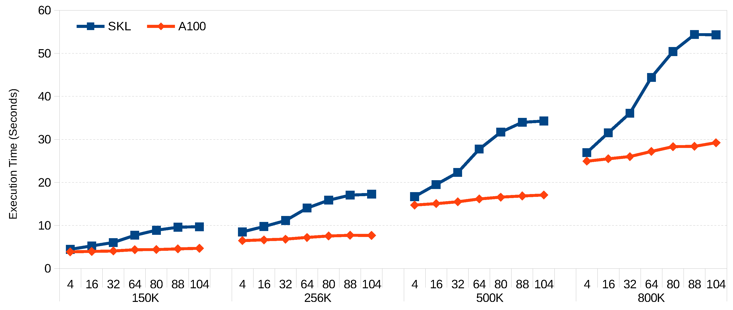
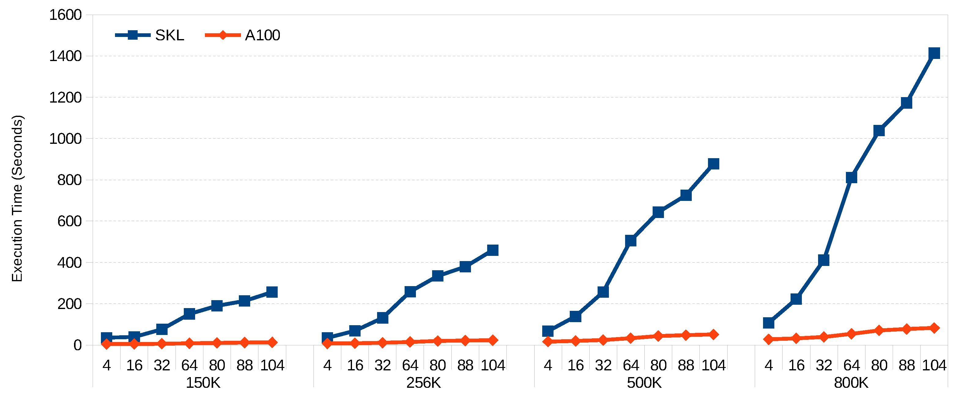
Figure 3 and Figure 4 show the scalability of FCM and GK-FCM, respectively, for big datasets. FM was excluded due to the long execution times for big datasets. In this case, we use the same hyper-ellipsoids but with increased rows (150 K, 256 K, 500 K, 800 K) and columns (80, 88 and 104). We can see that for both algorithms, the scalability with the number of columns (variables) is much better for the GPU. This is due to the fact that the SIMD extensions of the CPU can handle up to 8 double precision floating point per SIMD register, while the number of threads the GPU can handle is in the order of millions. Wider vector registers on the CPU would help to balance this trend. For example, ARM’s SVE can work with 2048-bit registers, compared with 512-bit registers of Intel’s AVX-512. On the other hand, scalability with row count is almost linear for both platforms. Increasing core count on the CPU would significantly reduce its execution time (our CPU only has 8 cores, and many servers have 64 cores). On the other hand, doubling the core count in a GPU would be difficult given the power it dissipates per unit area and the current GPU die sizes.

5.5. Discussion

This section discusses what are the best platforms and algorithms to run on, based on the datasets to analyse. First, let us break down the dataset type. If the dataset to run has an unknown number of clusters, FM is the best option as one of the its main features is that users do not need to set the number of cluster to obtain. For the FM algorithm, running on the CPU is faster and more energy efficient as long as the number of variables per entry is below 16. Otherwise, running on the GPU is faster, and consumes over 2.6× less energy. This is mainly due to the fact that the r factor computation is extremely compute intensive and highly parallelisable, meaning that the GPU has the advantage over the CPU as the dataset size increases and becomes the hotspot of the algorithm. Nevertheless, the update prototypes function requires the modification of a data structure in mutual exclusion, and for that purpose the CPU works best regardless of the input size. We leave as future work to design hybrid CPU-GPU implementation of FM. Nevertheless, FM is several orders of magnitude slower than the other clustering mechanisms for big datasets mainly due to the blind search of clusters previously commented.

On the other hand, if the number of clusters is known, and we are dealing with spherical clusters, FCM is the best alternative. FCM also works best on the CPU for datasets below 16 variables. However, GPUs are preferred in terms of performance for bigger datasets, but not in terms of power. This is mainly because the GPU is underutilised for FCM algorithm. Indeed, the extra idle power dissipated by the GPU does not pay off compared with the performance it provides. FCM parallelises on the row count for the CPU. Therefore, as the number of rows increases, the proportion of computation to communication time increases, meaning greater the energy benefits in favour of the CPU. Probably, a 16-core CPU with AVX-512 will outperform the GPU, in terms of performance and energy, regardless of the dataset size. Finally, GK-FCM is better suited if we are dealing with other clusters shapes. Computationally speaking, GK-FCM performs best on the GPU for almost all cluster sizes and variable count, and it is therefore the best platform to chose. A detailed profile of the CPU using Intel’s Vtune revealed an extremely low CPU utilisation. Most of the CPU time was spent in trivial data movements (e.g., transposition). SIMD extensions are not good at re-organising data in memory if there is no sequential pattern. Besides, SIMD helps for high column count. The increase on column count translates into an increment of the computation requirements. Therefore, the overhead of the transposition becomes less impact on the overall performance.

6. Conclusions and Future Work

Clustering algorithms are one of the most used algorithms to produce valuable knowledge in data science. These algorithms group a set of data elements (measures, points, patterns, etc.) into clusters. Their main characteristic is that individuals from a cluster are closer to its centre than to any other given cluster centre. This definition is extended in fuzzy clustering methods, where each data point can belong to more than one cluster. Typical examples of these algorithms include the Fuzzy C-means (FCM), Gustafson–Kessel FCM (GK-FCM) and the Fuzzy Minimals (FM). Given that the current trend in processor design moves towards heterogeneous and massively parallel designs, it becomes mandatory to redefine clustering algorithms to take full advantage of these architectures.

This article introduces several parallelisation strategies for clustering algorithms for both Intel and Nvidia-based architectures. Particularly, we focus on three widely applied fuzzy clustering techniques such as FCM, GK-FCM and FM. Parallel implementations are then evaluated in terms of performance and energy efficiency. Our results show that, if there is a need to compute a dataset with an unknown number of clusters, FM on CPU is the best option as long as the number of variables is below 16. If the number of clusters is known, and we are dealing with spherical clusters, FCM is the best alternative. FCM also works best on the CPU for datasets below 16 variables. However, for big datasets, a GPU is preferred in terms of performance, but not in terms of power. Finally, if we are dealing with other clusters shapes, GK-FCM is preferred. GK-FCM works best on the GPU for almost all cluster sizes and variable count, and it is therefore the best platform to chose.

Clustering algorithms are undoubtedly necessary in today’s computing landscape. Depending on the context, these algorithms must be efficient in both performance and consumption, therefore, in the future a middleware can be developed that depending on the constraints of the target platforms or its instantaneous workload, executes one or the other workload, knowing its possible deviations.

References

- Tagarev, T.; Atanasov, K.; Kharchenko, V.; Kacprzyk, J. Digital Transformation, Cyber Security and Resilience of Modern Societies; Springer Nature: Berlin/Heidelberg, Germany, 2021; Volume 84. [Google Scholar]
- Singh, D.; Reddy, C.K. A survey on platforms for big data analytics. J. Big Data 2015, 2, 8. [Google Scholar] [CrossRef] [PubMed] [Green Version]
- Intel Corporation. 2015. Available online: https://www.intel.es/content/www/es/es/architecture-and-technology/64-ia-32-architectures-software-developer-vol-2a-manual.html (accessed on 1 July 2021).
- ARM NEON Technology. 2012. Available online: https://developer.arm.com/architectures/instruction-sets/simd-isas/neon (accessed on 1 July 2021).
- Stephens, N.; Biles, S.; Boettcher, M.; Eapen, J.; Eyole, M.; Gabrielli, G.; Horsnell, M.; Magklis, G.; Martinez, A.; Premillieu, N.; et al. The ARM Scalable Vector Extension. IEEE Micro 2017, 37, 26–39. [Google Scholar] [CrossRef] [Green Version]
- Sodani, A. Knights Landing (KNL): 2nd Generation Intel Xeon Phi Processor. In Proceedings of the 2015 IEEE Hot Chips 27 Symposium (HCS), Cupertino, CA, USA, 22–25 August 2015. [Google Scholar]
- Yoshida, T. Introduction of Fujitsu’s HPC Processor for the Post-K Computer. In Proceedings of the 2016 IEEE Hot Chips 28 Symposium (HCS), Cupertino, CA, USA, 21–23 August 2016. [Google Scholar]
- NEC. Vector Supercomputer SX Series: SX-Aurora TSUBASA. 2017. Available online: http://www.nec.com/en/global/solutions/hpc (accessed on 7 January 2021).
- Wright, S.A. Performance Modeling, Benchmarking and Simulation of High Performance Computing Systems. Future Gener. Comput. Syst. 2019, 92, 900–902. [Google Scholar] [CrossRef]
- Gelado, I.; Garland, M. Throughput-oriented GPU memory allocation. In Proceedings of the 24th Symposium on Principles and Practice of Parallel Programming, Washington, DC, USA, 16–20 February 2019; pp. 27–37. [Google Scholar]
- Rodriguez, M.Z.; Comin, C.H.; Casanova, D.; Bruno, O.M.; Amancio, D.R.; Costa, L.d.F.; Rodrigues, F.A. Clustering algorithms: A comparative approach. PLoS ONE 2019, 14, e0210236. [Google Scholar] [CrossRef] [PubMed]
- Tan, P.; Steinbach, M.; Kumar, V. Introduction to Data Mining; Pearson Addison-Wesley: Boston, MA, USA, 2006. [Google Scholar]
- Jain, A.; Murty, M.Y.; Flynn, P. Data clustering: A review. ACM Comput. Surv. 1999, 31, 264–323. [Google Scholar] [CrossRef]
- Lee, J.; Hong, B.; Jung, S.; Chang, V. Clustering learning model of CCTV image pattern for producing road hazard meteorological information. Future Gener. Comput. Syst. 2018, 86, 1338–1350. [Google Scholar] [CrossRef] [Green Version]
- Cecilia, J.M.; Timón, I.; Soto, J.; Santa, J.; Pereñíguez, F.; Muñoz, A. High-Throughput Infrastructure for Advanced ITS Services: A Case Study on Air Pollution Monitoring. IEEE Trans. Intell. Transp. Syst. 2018, 19, 2246–2257. [Google Scholar] [CrossRef]
- Bueno-Crespo, A.; Soto, J.; Muñoz, A.; Cecilia, J.M. Air-Pollution Prediction in Smart Cities through Machine Learning Methods: A Case of Study in Murcia, Spain. J. Univ. Comput. Sci. 2018, 24, 261–276. [Google Scholar]
- Pérez-Garrido, A.; Girón-Rodríguez, F.; Bueno-Crespo, A.; Soto, J.; Pérez-Sánchez, H.; Helguera, A.M. Fuzzy clustering as rational partition method for QSAR. Chemom. Intell. Lab. Syst. 2017, 166, 1–6. [Google Scholar] [CrossRef]
- Jain, A.K. Data clustering: 50 years beyond k-means. Pattern Recognit. Lett. 2010, 31, 651–666. [Google Scholar] [CrossRef]
- Gan, G.; Ma, C.; Wu, J. Data Clustering: Algorithms and Applications; Chapman and Hall/CRC Data Mining and Knowledge Discovery Series; CRC: Boca Raton, FL, USA, 2013. [Google Scholar]
- Bezdek, J.C.; Ehrlich, R.; Full, W. FCM: The Fuzzy C-Means clustering algorithm. Comput. Geosci. 1984, 10, 191–203. [Google Scholar] [CrossRef]
- Gustafson, D.E.; Kessel, W.C. Fuzzy clustering with a fuzzy covariance matrix. In Proceedings of the 1978 IEEE Conference on Decision and Control Including the 17th Symposium on Adaptive Processes, Ft. Lauderdale, FL, USA, 12–14 December 1979; pp. 761–766. [Google Scholar]
- Flores-Sintas, A.; Cadenas, J.M.; Martín, F. A local geometrical properties application to fuzzy clustering. Fuzzy Sets Syst. 1998, 100, 245–256. [Google Scholar] [CrossRef]
- Soto, J.; Flores-Sintas, A.; Palarea-Albaladejo, J. Improving probabilities in a fuzzy clustering partition. Fuzzy Sets Syst. 2008, 159, 406–421. [Google Scholar] [CrossRef]
- Shehab, M.A.; Al-Ayyoub, M.; Jararweh, Y. Improving fcm and t2fcm algorithms performance using gpus for medical images segmentation. In Proceedings of the 2015 6th International Conference on Information and Communication Systems (ICICS), Amman, Jordan, 7–9 April 2015; pp. 130–135. [Google Scholar]
- Cecilia, J.M.; Cano, J.C.; Morales-García, J.; Llanes, A.; Imbernón, B. Evaluation of clustering algorithms on GPU-based edge computing platforms. Sensors 2020, 20, 6335. [Google Scholar] [CrossRef]
- Saxena, A.; Prasad, M.; Gupta, A.; Bharill, N.; Patel, O.P.; Tiwari, A.; Er, M.J.; Ding, W.; Lin, C.T. A review of clustering techniques and developments. Neurocomputing 2017, 267, 664–681. [Google Scholar] [CrossRef] [Green Version]
- Ahmed, M.; Seraj, R.; Islam, S.M.S. The k-means algorithm: A comprehensive survey and performance evaluation. Electronics 2020, 9, 1295. [Google Scholar] [CrossRef]
- Hou, X. An Improved K-means Clustering Algorithm Based on Hadoop Platform. In The International Conference on Cyber Security Intelligence and Analytics; Springer: Berlin/Heidelberg, Germany, 2019; pp. 1101–1109. [Google Scholar]
- Zhao, Q.; Shi, Y.; Qing, Z. Research on Hadoop-based massive short text clustering algorithm. In Fourth International Workshop on Pattern Recognition; International Society for Optics and Photonics: Nanjing, China, 2019; Volume 11198, p. 111980A. [Google Scholar]
- Xiong, H. K-means Image Classification Algorithm Based on Hadoop. In Recent Developments in Intelligent Computing, Communication and Devices; Springer: Berlin/Heidelberg, Germany, 2019; pp. 1087–1092. [Google Scholar]
- Jin, C.; Patwary, M.M.A.; Agrawal, A.; Hendrix, W.; Liao, W.k.; Choudhary, A. DiSC: A distributed single-linkage hierarchical clustering algorithm using MapReduce. Work 2013, 23, 27. [Google Scholar]
- Woodley, A.; Tang, L.X.; Geva, S.; Nayak, R.; Chappell, T. Parallel K-Tree: A multicore, multinode solution to extreme clustering. Future Gener. Comput. Syst. 2019, 99, 333–345. [Google Scholar] [CrossRef]
- Kwedlo, W.; Czochanski, P.J. A Hybrid MPI/OpenMP Parallelization of K-Means Algorithms Accelerated Using the Triangle Inequality. IEEE Access 2019, 7, 42280–42297. [Google Scholar] [CrossRef]
- Li, Y.; Zhao, K.; Chu, X.; Liu, J. Speeding up k-means algorithm by gpus. J. Comput. Syst. Sci. 2013, 79, 216–229. [Google Scholar] [CrossRef]
- Saveetha, V.; Sophia, S. Optimal tabu k-means clustering using massively parallel architecture. J. Circuits Syst. Comput. 2018, 27, 1850199. [Google Scholar] [CrossRef]
- Djenouri, Y.; Djenouri, D.; Belhadi, A.; Cano, A. Exploiting GPU and cluster parallelism in single scan frequent itemset mining. Inf. Sci. 2019, 496, 363–377. [Google Scholar] [CrossRef]
- Krawczyk, B. GPU-accelerated extreme learning machines for imbalanced data streams with concept drift. Procedia Comput. Sci. 2016, 80, 1692–1701. [Google Scholar] [CrossRef] [Green Version]
- Karbhari, S.; Alawneh, S. GPU-Based Parallel Implementation of K-Means Clustering Algorithm for Image Segmentation. In Proceedings of the 2018 IEEE International Conference on Electro/Information Technology (EIT), Rochester, MI, USA, 3–5 May 2018; pp. 52–57. [Google Scholar]
- Jagtap, S.V.; Rao, Y. Clustering and Parallel Processing on GPU to Accelerate Circuit Transient Analysis. In International Conference on Advanced Computing Networking and Informatics; Springer: Berlin/Heidelberg, Germany, 2019; pp. 339–347. [Google Scholar]
- Fang, Y.; Chen, Q.; Xiong, N. A multi-factor monitoring fault tolerance model based on a GPU cluster for big data processing. Inf. Sci. 2019, 496, 300–316. [Google Scholar] [CrossRef]
- Tanweer, S.; Rao, N. Novel Algorithm of CPU-GPU hybrid system for health care data classification. J. Drug Deliv. Ther. 2019, 9, 355–357. [Google Scholar] [CrossRef] [Green Version]
- Zadeh, L.A.; Klir, G.J.; Yuan, B. Fuzzy Sets, Fuzzy Logic, and Fuzzy Systems: Selected Papers; World Scientific: London, UK, 1996; Volume 6. [Google Scholar]
- Anderson, D.T.; Luke, R.H.; Keller, J.M. Speedup of fuzzy clustering through stream processing on graphics processing units. IEEE Trans. Fuzzy Syst. 2008, 16, 1101–1106. [Google Scholar] [CrossRef]
- Al-Ayyoub, M.; Abu-Dalo, A.M.; Jararweh, Y.; Jarrah, M.; Al Sa’d, M. A gpu-based implementations of the fuzzy c-means algorithms for medical image segmentation. J. Supercomput. 2015, 71, 3149–3162. [Google Scholar] [CrossRef]
- Aaron, B.; Tamir, D.E.; Rishe, N.D.; Kandel, A. Dynamic incremental fuzzy C-means clustering. In Proceedings of the Sixth International Conference on Pervasive Patterns and Applications, Venice, Italy, 25–29 May 2014; pp. 28–37. [Google Scholar]
- Téllez-Velázquez, A.; Cruz-Barbosa, R. A CUDA-streams inference machine for non-singleton fuzzy systems. Concurr. Comput. Pract. Exp. 2018, 30, e4382. [Google Scholar] [CrossRef]
- Cebrian, J.M.; Imbernón, B.; Soto, J.; García, J.M.; Cecilia, J.M. High-throughput fuzzy clustering on heterogeneous architectures. Future Gener. Comput. Syst. 2020, 106, 401–411. [Google Scholar] [CrossRef]
- Scully-Allison, C.; Wu, R.; Dascalu, S.M.; Barford, L.; Harris, F.C. Data Imputation with an Improved Robust and Sparse Fuzzy K-Means Algorithm. In Proceedings of the 16th International Conference on Information Technology-New Generations (ITNG 2019); Springer: Berlin/Heidelberg, Germany, 2019; pp. 299–306. [Google Scholar]
- Graves, D.; Pedrycz, W. Fuzzy C-Means, Gustafson-Kessel FCM, and Kernel-Based FCM: A Comparative Study. In Analysis and Design of Intelligent Systems using Soft Computing Techniques; Springer: Berlin/Heidelberg, Germany, 2007; pp. 140–149. [Google Scholar] [CrossRef]
- Timón, I.; Soto, J.; Pérez-Sánchez, H.; Cecilia, J.M. Parallel implementation of fuzzy minimals clustering algorithm. Expert Syst. Appl. 2016, 48, 35–41. [Google Scholar] [CrossRef]
- Pedrycz, W. Fuzzy Clustering. In An Introduction to Computing with Fuzzy Sets: Analysis, Design, and Applications; Springer International Publishing: Cham, Switzerland, 2021; pp. 125–145. [Google Scholar] [CrossRef]
- de la Hermosa González, R.R. Wind farm monitoring using Mahalanobis distance and fuzzy clustering. Renew. Energy 2018, 123, 526–540. [Google Scholar] [CrossRef]
- Krishnapuram, R.; Kim, J. A note on the Gustafson-Kessel and adaptive fuzzy clustering algorithms. IEEE Trans. Fuzzy Syst. 1999, 7, 453–461. [Google Scholar] [CrossRef]
- Flores-Sintas, A.; Cadenas, J.M.; Martín, F. Detecting homogeneous groups in clustering using the euclidean distance. Fuzzy Sets Syst. 2001, 120, 213–225. [Google Scholar] [CrossRef]
- Guennebaud, G.; Jacob, B. Eigen v3.4. 2010. Available online: http://eigen.tuxfamily.org (accessed on 1 July 2021).
Figure 1.
Speed-up (normalised to scalar code running on one thread).
Figure 2.
Energy reduction factor (normalised to scalar code running on one thread).
Figure 3.
Execution time (seconds) for FCM.
Figure 4.
Execution time (seconds) for GK-FCM.
Publisher’s Note: MDPI stays neutral with regard to jurisdictional claims in published maps and institutional affiliations. |
© 2021 by the authors. Licensee MDPI, Basel, Switzerland. This article is an open access article distributed under the terms and conditions of the Creative Commons Attribution (CC BY) license (https://creativecommons.org/licenses/by/4.0/).
Share and Cite
MDPI and ACS Style
Cebrian, J.M.; Imbernón, B.; Soto, J.; Cecilia, J.M. Evaluation of Clustering Algorithms on HPC Platforms. Mathematics 2021, 9, 2156. https://0-doi-org.brum.beds.ac.uk/10.3390/math9172156
AMA Style
Cebrian JM, Imbernón B, Soto J, Cecilia JM. Evaluation of Clustering Algorithms on HPC Platforms. Mathematics. 2021; 9(17):2156. https://0-doi-org.brum.beds.ac.uk/10.3390/math9172156
Chicago/Turabian StyleCebrian, Juan M., Baldomero Imbernón, Jesús Soto, and José M. Cecilia. 2021. "Evaluation of Clustering Algorithms on HPC Platforms" Mathematics 9, no. 17: 2156. https://0-doi-org.brum.beds.ac.uk/10.3390/math9172156
Note that from the first issue of 2016, this journal uses article numbers instead of page numbers. See further details here.