
Representing Integer Sequences Using Piecewise-Affine Loops


1
CITIC, Computer Architecture Group, Universidade da Coruña, 15071 A Coruña, Spain
2
Department of Computer Science, Colorado State University, Fort Collins, CO 80523, USA
*
Author to whom correspondence should be addressed.
Mathematics 2021, 9(19), 2368; https://0-doi-org.brum.beds.ac.uk/10.3390/math9192368
Submission received: 17 July 2021
/
Revised: 14 September 2021
/
Accepted: 18 September 2021
/
Published: 24 September 2021
(This article belongs to the Special Issue Current Trends in Computer Architecture and High Performance Computing (HPC) with Their Mathematical Foundations)
Abstract
:A formal, high-level representation of programs is typically needed for static and dynamic analyses performed by compilers. However, the source code of target applications is not always available in an analyzable form, e.g., to protect intellectual property. To reason on such applications, it becomes necessary to build models from observations of its execution. This paper details an algebraic approach which, taking as input the trace of memory addresses accessed by a single memory reference, synthesizes an affine loop with a single perfectly nested reference that generates the original trace. This approach is extended to support the synthesis of unions of affine loops, useful for minimally modeling traces generated by automatic transformations of polyhedral programs, such as tiling. The resulting system is capable of processing hundreds of gigabytes of trace data in minutes, minimally reconstructing 100% of the static control parts in PolyBench/C applications and 99.99% in the Pluto-tiled versions of these benchmarks. As an application example of the trace modeling method, trace compression is explored. The affine representations built for the memory traces of PolyBench/C codes achieve compression factors of the order of and with respect to gzip for the original and tiled versions of the traces, respectively.
1. Introduction
Code analyses and optimizations usually work on top of the application code. Unfortunately, source codes are oftentimes not accessible for analysis. Whether due to licensing, privacy, obfuscation, or even access to the execution environment, users have to work on post-mortem execution logs, such as memory access traces, which prevents seamless static analysis. Even if the source code is available, it may use complex data and control structures, including code obfuscation [1], making it not amenable to static analysis. In sparse computations, indirection arrays are used for accessing data, hiding the potential regularity inherent in the sparsity structure [2]. In all these domains, the generation of compact closed-forms from a trace of integers allows us to generate code analyzable using classical techniques. Note that all these problems are equivalent to the reconstruction of the code of a memory reference from its access trace, and that is the form in which the problem is discussed in the following.
This paper presents an analytical approach for automatically building piecewise-affine references that model a sequence of arbitrary integer values. Affine codes [3] are a subclass of programs that execute large, regular loops, where both instruction- and data-flow depend only on loop induction variables and constant values. Fundamental kernels extracted from all computing domains, from supercomputing to embedded systems, including multimedia, can be represented using this abstraction, and treated using polyhedral optimizers [4,5]. The Trace Reconstruction Engine (TRE) traverses a space in which each node encodes an affine loop. Level k contains the nodes that represent all the canonical affine loops of dimensionality lesser or equal than k whose trip count is equal to k, starting from a 1-level nest which iterates from 0 to , and ending on a k-level nest with a single iteration per level. TRE works by analyzing the memory trace, building equation systems that compute iteration polyhedra and access functions that reproduce the access strides observed in the trace. This work analyzes the tractability of employing different exploration strategies for analyzing iteration spaces with increasing complexities. The main contributions of this work are:
- A detailed mathematical formulation for the automatic construction of an affine representation of a sequence of integers using increasingly complex representations. Simple affine domains are explored first (Section 3), and the formulation is later generalized to explore the general case of piecewise-affine domains, featuring multiple lower and upper iteration bounds at each nesting level (Section 4).
- While the space of simple polyhedra can be efficiently explored using brute force, more complex, piecewise-affine spaces are much larger and require costly algebraic computations to explore, introducing the need for parallel heuristic exploration techniques in order to make the problem tractable (Section 4.4).
- A detailed experimental evaluation of the proposed techniques when reconstructing traces using only a single canonical iteration domain, i.e., a single loop nest where lower and upper loop bounds are defined by a single affine expression (Section 3.6), and on piecewise-affine codes (Section 4.6). Our results show that the framework can be used to reconstruct large, complex traces in acceptable time.
Besides efficient trace compression, the framework can potentially be applied to guide all sorts of static and dynamic analyses and optimizations in the absence of source and/or binary codes, or when working with codes that are not amenable to static analysis for any reason. Examples of applications are hardware and software prefetching, data placement for locality optimizations, dependence analysis for automatic parallelization, optimal design of embedded memory systems for locality, or piecewise-regular code generation for sparse codes. These applications are discussed in depth in Section 5, along with the related work.
This article is a revision and extension of previous works [6,7]. In the former, the authors covered the reconstruction of single-domain affine traces with integer constraints only. The latter introduces some results and intuitions for the extension to the piecewise-affine model. The current work presents the full mathematical formulation that handles the general class of unions of affine domains. It discusses in detail the mathematical properties of the trace reconstruction algorithm. The experimental section is greatly extended, incorporating a full analysis of the computability of the trace reconstruction for different types of programs, and revamping the execution environments and platforms to take advantage of new optimizations and more powerful hardware.
2. Problem Formulation
The trace of memory locations accessed by a program can be considered an arbitrary sequence of integers. During the execution, this sequence will include accesses generated by many different instructions, including multiple loop scopes. This work assumes that each entry in the trace is labeled using a unique identifier for the instruction that issued the address. An example of this trace format is the one generated by Intel’s Pin Tool [8]. The unique label allows us to analyze the sequence of integers generated by each instruction separately. Related works have proposed ways to single out loop sections in the trace [9,10], which can be used if a single instruction may appear in different loop scopes. The proposed algorithm focuses on the individual reconstruction of each reference. Optimizations requiring cross-reference analysis would require a post-processing step to recombine the different streams considering their respective scopes. This post-processing is out of the scope of this paper.
While subsequent sections will extend the proposal to the general class of piecewise-affine loops, to introduce the problem and its mathematical formulation, we initially focus on the subclass of single-domain integer affine loops. Without loss of generality, these can be written as:
where are affine functions with integer coefficients (We use to simplify notation, even though we should formally write . It is assumed that coefficients of out-of-scope indices are 0); , is the set of affine functions that converts a given point in the iteration space of the nest to a point in the data space of V; and is a column vector that encodes the state of each iteration variable for the execution of V. The complete access is abbreviated by . Iteration bounds are assumed to be inclusive. Since is affine, the access can be rewritten as:
where V is the base address of the array, is a constant stride, and each is the coefficient of the loop index , and must account for the dimensionality of the original array (For instance, an access to an array can be rewritten as , where accounts for both the constant multiplying i in the original access (2), and the size of the fastest changing dimension (M)). This is the canonical form into which the method proposed in this paper reconstructs single-domain loops. In the following, the term “affine loop” will refer to a single-domain integer affine loop, while more general types such as piecewise-affine loops or loops defined using rational coefficients will be explicitly identified as such. These more general types of loops are formally described and covered in Section 4.
| DO = 0, |
| ⋮ |
| DO = 0, |
During the execution of the loop nest, the access to V will orderly issue the addresses corresponding to , , etc. These addresses will be registered in the trace file together with the instruction issuing them and the size of the accessed data.
Geometrical Considerations
Using the polyhedral model, each iteration of a loop is represented as a point in a D-dimensional space. Inside this infinite space, the set of legal iterations of the loop is contained by an integer polyhedron of dimension D. The polyhedron is defined as the intersection of a collection of half-planes defined by affine inequalities. Each inequality corresponds to a lower or upper bound of an iteration index of the loop. Geometrically, each inequality constitutes one of the F faces of the iteration polyhedron. In particular, an affine loop such as the one previously studied corresponds to a polyhedron with D dimensions and faces. Faces corresponding to lower or upper bounds have linear inequations of the forms and , respectively. In the following, we will refer to these as the lower/upper bounds hyperplanes.
Consider two consecutive accesses, and , and assume that the loop index values in and the upper bounds functions are known. The values in can be computed as follows:
- According to common programming language rules, an index will reset to 0 when it reaches its upper bound only if all inner ones have also reached their respective upper bounds. This can be expressed as:The geometrical interpretation is that lies on the edge formed by the union of the upper bounds hyperplanes of the iteration polyhedron for dimension j and inner dimensions .
- According to common programming language rules, an index will increase by 1 when all inner loops have reached their respective upper bounds, but the loop at level j has not. This can be expressed as:The geometrical interpretation is that lies on the edge formed by the union of the upper bounds hyperplanes of the iteration polyhedron for inner dimensions , but not on the hyperplane which serves as the upper bounds for dimension j.
- In any other case, index will not change, i.e., .
Definition 1.
A set of indices built complying with these conditions will be referred to as a set of sequential indices.
Corollary 1.
The instantaneous variation of loop indexbetween iterations k and, , can only take one of three possible values:
- 1.
- Ifis reset to 0;
- 2.
- Ifis increased by one;
- 3.
- Ifdoes not change.
Lemma 1.
The stride between two consecutive accessesis a linear combination of the coefficients of the loop indices.
Proof.
Using Equation (1), can be rewritten as:
□
The class of loops described in this section can model most hand-written affine memory references and, in particular, all the memory references in the PolyBench/C benchmarks [11]. Section 3 presents an approach to reconstruct single-domain affine loops using the minimal possible dimension of the iteration space. Section 4 studies the more complex problem of reconstructing the general class of piecewise-affine loops. These are rarely used in hand-written codes, but very commonly appear after applying automated optimizations to single-domain loops, such as loop tiling [12,13].
3. Modeling Single-Domain References
The approach proposed in order to reconstruct single-domain loops consists in systematically exploring the solution space, using the access strides of a given instruction, computed as the first-order differences of the integer sequence, as the exploration guide. Each node in the solution space encodes an affine loop, which tries to reconstruct a portion of the entire trace. For each node, its children represent the affine loops in which a single iteration has been added with respect to their parent. Figure 1 shows a geometrical view of these concepts, and Figure 2 presents a symbolic view.
The root of this solution space is a trivial one-iteration loop, which generates the first two entries in the memory trace. The Trace Reconstruction Engine (TRE) traverses the solution space, adding one access to the candidate loop in each step, until reaching a candidate loop that generates the entire sequence of integers in the trace, or concludes that no affine loop may generate the input. The TRE may not build a solution with the same dimensionality as the original code. More precisely, it builds the nest with the minimal dimension required to generate the observed sequence of accesses. For example, a 2-level loop with indices i and j might iterate sequentially over the elements in array if the upper bounds are defined as , and the access is . This can be rewritten as a 1-level loop with index i, using and access . This section presents strategies to efficiently explore the solution space towards this node, exploiting the mathematical properties of the problem.
Let be the sequence of addresses generated by a single reference in a single loop scope, extracted from the execution trace. The reconstruction algorithm iteratively constructs a solution , which generates using D nested loops. The components of this solution are defined as follows:
- Vector of coefficients of loop indices.
- Matrix , and vector , the upper bounds matrix and vector, respectively. Any single-domain affine loop can be rewritten to have lower bounds functions , and therefore it is not necessary to explicitly store them.
The iteration domain is an integer polyhedron containing the iteration vectors such that:
where can be arranged in a lower triangular fashion, since no index may depend on the index of an inner loop. Its main diagonal is equal to . Its row, , contains the coefficients of each loop index in the affine bounds function , while contains its independent term. Together, they encode the upper bounds as .
To be a valid solution, its generated access strides must match the observed ones in the trace. Using Lemma 1 this can be expressed as:
The algorithm proceeds iteratively, constructing partial solutions for incrementally larger parts of the trace . The first partial solution is built as:
or, equivalently:
| DO = 0, 1 |
Consider the source code of the cholesky application from the PolyBench/C suite [11] in Figure 3. For the sake of clarity, in this example we will only focus on the analysis of the access A[i][k] in line 11. An excerpt of its memory trace is shown in Figure 4. The first partial solution, which reconstructs the subtrace , is found to be:
Starting from this first partial solution the engine begins exploring the solution space, adding one element to the trace in each step, until it arrives at a full solution for . In each step, the algorithm processes access , calculating the observed access stride, , and building a diophantine linear equation system according to Lemma 1 to compute the candidate indices , which result in an access stride equal to the observed one:
where is the system matrix, and is the solution. There are two possible situations when solving this system:
- The system has one or more integer solutions. In this case, for each solution , the new index , which must be sequential to , is calculated. and remain unchanged. Each of these solutions, whose calculation is detailed in Section 3.1, must be explored independently as described in Section 3.3.
- The system has no solution generating an index sequential to , in which case there are three courses of action:
- (a)
- Increase the dimensionality D (Section 3.2).
- (b)
- Modify the bounds and (Section 3.4).
- (c)
- Discard the solution and backtrack.
3.1. Efficiently Solving the Linear Diophantine System
Although the system in Equation (4) has infinite solutions in the general case, only a few are valid in the context of affine loop reconstruction, which makes it possible to develop very efficient ad hoc solution strategies.
Lemma 2.
There are at most D valid solutions to the system in Equation (4). These correspond to indices:
Proof.
If index must be sequential to index as per Definition 1, then there is a single degree of freedom for : the position that is equal to 1.
Positions will not change between iterations k and , and therefore ; while positions will be reset to 0, and therefore . □
Taking this result into account, it is possible to find all valid solutions of the system in linear time, , by simply testing the D valid candidates , calculating their associated strides , and accepting those solutions with a stride equal to the observed one, . These are particular solutions of the subtrace , which will be explored to construct a solution for the entire trace.
Following the example, the next access in the trace to be processed is . The engine computes the access stride as . At this point, a 1-level loop has been constructed and the engine checks whether produces a stride that matches the observed one. The equality holds, and the solution is accepted. The algorithm continues processing the trace until it builds , with . At this point, the observed stride changes to:
The constructed loop with cannot produce a stride different from 0. As such, the subtrace cannot be generated with an affine access enclosed in a 1-level loop and the dimensionality of the current solution must be increased to build .
3.2. Increasing Solution Dimensionality
Let be a partial solution for the subtrace . If no valid index in provides , it may be because a loop index that had not appeared before is increasing in access . This can cause to be unrepresentable either as a linear combination of the loop coefficients , or through an index sequential to . It is always possible to generate at least valid partial solutions from by enlarging the dimensionality of the current solution components. These solutions correspond to the indices . For each insertion position p of the newly discovered loop, the set of indices , is built as matrix:
where a 0 in position p has been added to each index in , and a new column has been added to the matrix. The coefficient associated with the new loop index can be derived from Equation (4):
and are updated as described in Section 3.4 to reflect the new information available. If no solution is found for the boundary conditions, then the generated polyhedron is not convex and this branch is discarded. However, at least the insertion point , i.e., adding a new outer loop to the nest, will always have affine associated bounds. Note that there must be a practical limit to the maximum acceptable solution size, as in the general case any trace can be generated using at most affine nested loops with integer coefficients. To ensure that a minimal solution, in terms of the dimensionality of the generated –polyhedron, is found, the solution space should be traversed in a breadth-first fashion.
Revisiting the example, there are two possible insertion points for the new loop in . As the most common situation is that newly discovered loops are outer than the previously known ones, it explores first. The new loop coefficient vector and iteration polyhedron are calculated as:
The traversal of the solution space continues. The next observed stride is . No increase of the currently found loop indices produces such a stride:
Hence, the solution must grow to . Now, there are three different insertion points. The first two yield the following coefficient vectors:
As soon as the first points are explored in these branches, the engine will find that further dimensionality increases are necessary to model the entire trace. Due to the breadth-first nature of the exploration, it will then backtrack to the third possible insertion point:
At this stage the engine has correctly calculated the coefficients of the three levels of the original nest. It generates the new iteration polyhedron:
For the sake of simplicity, this section does not discuss the calculations associated to loop bounds. These will be detailed in Section 3.4.
3.3. Branch Priority
The approach proposed above is capable of efficiently finding the relevant solutions of the linear Diophantine system for each address of the trace, but can still produce a large number of potential solutions that will be discarded when processing the remaining addresses in the trace. In the general case, the time for exploring the entire solution space of a trace containing P addresses generated by D loops would be . Consequently, exploring all branches is not a tractable problem in the general case. To guide the traversal of the solution space, consider the column vector defined as:
Lemma 3.
Each elementindicates how many more iterations of indexare left before it resets under bounds, .
Proof.
is equal to the value of the upper bounds of the loop in minus the current value of or, equivalently, to the distance from to the upper bounds face associated to index :
By construction of the canonical loop form, the step of all loops is 1. Therefore, is equal to the number of iterations of loop before . □
This result suggests that, assuming that and are accurate, the most plausible value for the next index is , where l is the position of the innermost positive element of . The correctness of this prediction can be assessed by comparing the predicted stride with the observed one . Note that using as described above guarantees consistency with the boundary conditions in Equation (2), which further improves the efficiency of the approach by saving calculations.
3.4. Calculating Loop Bounds
So far, the calculation of the boundary conditions, and , has been overlooked. As before, assume that the algorithm has already identified a partial solution . Upon processing access , the algorithm will try to explore the branch, which increments the index corresponding to the innermost positive element of , as described in Section 3.3. However, it might happen that the calculated stride for the selected branch does not match the observed stride, i.e., . A different candidate index will have to be generated as described in Section 3.1, but the resulting will not be sequential to under bounds and . In this scenario, it is necessary to generate new upper bounds and for all inner indices that were not expected to reset, i.e., (). Each of these hyperplanes must: (i) contain , so that index resets after ; (ii) contain the z indices that lay on the previous upper bounds hyperplane defined by and , to preserve the sequentiality in ; and (iii) leave all iteration vectors in beneath it, to guarantee polyhedron convexity. Mathematically, we are looking to build a matrix row and associated fulfilling two conditions:
where is a matrix with columns: , and the z iteration vectors lying on the previous upper bounds hyperplane, as per (i) and (ii) above. Besides, there are two structural constraints on the values of :
- , i.e., this hyperplane is associated to a function of type .
- , i.e, does not depend on iteration indices inner than j.
This problem is solved using integer linear programming [14] through the piplib library [15]. First, we solve Equation (6), building the hyperplane containing . Note that it is only necessary to choose at most j linearly independent columns from to build the equation system, as points in are cohyperplanar by definition. Afterwards, if any point in lies beyond this hyperplane, we iteratively modify the face so that it contains the point furthest away from it (in a way similar to Quickhull [16]). This process repeats until either a solution satisfying both Equations (6) and (7) is found; otherwise there is no convex polyhedron containing all points in , and and lie on one of its faces (i.e., this iteration sequence is not generated by an affine loop).
One possible solution to this underdetermined system is:
The calculated bounds are shown in Figure 5a. Continuing the example, , and the engine predicts , which generates a stride that matches the observed one. and the engine predicts , which also generates a stride that matches the observed one. This process continues, alternating iterations of and , until access is incorporated to the solution, with index . At this point, , and an iteration of is predicted, with . However, . The engine defaults to the brute force mode, calculating the strides for each of the currently known indices (see Section 3.1):
The engine explores the path with , and the loop bounds have to be updated:
The first and third rows of do not change. For the second, the following system is solved:
and the new upper bounds hyperplanes:
The resulting geometric bounds are depicted in Figure 5b. All the necessary information to solve the problem has been collected. From this point on, the engine will keep incorporating elements in the trace to the solution, with accurately predicting all the remaining iterations, until it reaches the end of the trace having reconstructed the following terms:
Note that this reconstruction method does not regenerate the constant term in Equation (1), and assumes the base address of the access to be . This is not a problem for any practical application of the constructed affine model, as the set of accessed points is identical to that of the original, potentially non-canonical loop.
3.5. Algorithm
Algorithm 1 presents the pseudocode of the Extract() function, which implements the Trace Reconstruction Engine (TRE) for modeling traces as single-domain integer affine loops. The recursive solution is not practical for a real implementation, but clearly illustrates the idea. The computations to calculate the new loop insertions described in Section 3.2 are encapsulated into a Grow() function, shown as Algorithm 2. The reconstruction starts by calling Extract() with the initial defined in Equation (3). In the worst case, when no access is correctly predicted using , the algorithm uses the brute force approach . In the best case, every access is correctly predicted ().
| Algorithm 1: Pseudocode of Extract(). |
 |
The TRE implementation loads into memory: (i) the input trace; (ii) , , and for each explored node in the solution space; and (iii) matrix for the current node being explored. The largest of these structures is , and so the consumed memory can be bound as . Other temporaries, e.g., equation systems, do not store more than a few dozen values, and so their memory consumption is not relevant. Note that the full trace will not reside into memory at any time during the reconstruction process. The trace is explored on a point-by-point basis, and therefore the virtual memory subsystem will dynamically load the relevant parts of the trace on demand.
| Algorithm 2: Pseudocode of Grow() (Section 3.2). | |
| Input: | the partial solution , the insertion point x, and the iteration polyhedron |
| Output: | modified partial solution and iteration polyhedron with a new loop in position x, or if the insertion point generates a nonlinear solution |
|
//
Insert a new row and column in
; // Insert a new element in ; // Insert new index into ; = update bounds // (Section 3.4) ; 6 if is not affine then return ; 7 return ; | |
3.6. Performance of Single-Domain Trace Reconstruction
The reference implementation of the TRE has been tested with all benchmarks included in the PolyBench/C 4.2.1 suite [11]. PolyBench contains 30 applications from different computational domains, such as linear algebra, data mining, or stencil codes. The proposed approach was applied to one reference for each loop scope in each SCoP (i.e., the main computational kernel of each application). All benchmarks were executed using -DLARGE_DATASET, except for floyd-warshall, which performs a number of memory accesses one order of magnitude larger than the second largest benchmark, and was executed using -DMEDIUM_DATASET. Table 1 details the characteristics of each test input trace. Each execution was performed on an AMD Ryzen 9 5950X, equipped with 128 GB of RAM.
Figure 6 details the performance obtained for the reconstruction of these single-domain kernels. The upper bar shows the reconstruction time in seconds, while the lower one shows trace sizes in number of entries. The performance obtained for each specific trace depends on the depth and the structure of the reconstructed loops. The best performance is obtained for one of the deriche subtraces, an edge detection filter accessing arrays with a constant, single stride. A single-strided trace is trivial to reconstruct, and this one is processed at more than 14 billion elements per second. If single-strided references are not taken into account, the most efficient processing is observed for one of the fdtd-2d references, a 2D finite-difference time-domain kernel. In the original code, this reference is written as a 3D loop, but is reconstructed by TRE as a 2D nest, as the two inner loops are coalesced into a single one. The outer loop trips once per each 1.2 million iterations of the inner one. In these cases, the reconstruction is streamlined: the trace contains single-strided blocks of 1.2 million elements, which are trivially predicted by and processed in a single step. The 600 million accesses in this subtrace are processed in 14 ms, i.e., at a rate of 4.3 billion elements per second.
The worse performance is observed for one of the references in doitgen, containing 3.4 million entries. It is generated by a 2D loop where the largest single-strided block contains 160 elements only. In this case, the number of steps performed during the reconstruction process is much larger, resulting in a reconstruction rate of only 2.1 million elements per second, i.e., 2000× slower than the fastest non-single-strided case. The aggregated input is processed at an average rate of 25.4 million accesses per second.
Regarding memory requirements, the exploration engine strictly needs to store only , , and the last reconstructed index . To improve performance reconstruction, the reference implementation also stores points in the convex hull of the iteration polytope, which are necessary for loop bounds recomputation, but could be recalculated on demand from the bounds equations for minimal memory consumption. The total storage requirements for the references in our experimental set vary between 48 bytes and 44 kB.
One simple application of the affine model is compressing the input memory trace. We compared raw sizes, sizes using NumPy’s NPZ (which uses gzip), and the sizes required to store , , and , which are enough to reconstruct the entire trace. The entire experimental set, which is 230 GB in size and can be compressed into 14.5 GB using , takes up 14 kB when compressed using the affine loop bounds reconstructed by the TRE. This represents a and compression factor with respect to the raw data and NPZ, respectively.
4. Modeling Piecewise-Affine References
The previously proposed formulation reconstructs traces using a single canonical loop nest. These are represented by the subspace of polyhedra with D dimensions and faces in which extreme points inside the polyhedron lie exactly on its bounding hyperplanes. However, many domains are represented using more complex polyhedra, with faces and/or as piecewise-affine union of polyhedra. These correspond to the general case of polyhedral programs, which can be described as:
| DO = , |
| ⋮ |
| DO = , |
where the number of faces F corresponds to, at most, the number of affine functions used to define the lower and upper bounds of each loop; and coefficients are rational, i.e., . The mathematical representation presented in Section 2 and Section 3 can be extended to cover this general case. For single-domain loops, the bounds matrix was defined as a matrix containing only the upper bounds faces of the polyhedron. Explicit representation of lower bounds faces was unnecessary, as the canonical form of these loops is represented by an iteration polyhedron such that all lower bounds faces lie exactly across one of the canonical axes, i.e., no negative components may exist in iteration vectors and the first iteration of all loops is always zero. As such, the equation implicitly incorporates lower bounds faces and the polyhedron:
is actually equivalent to:
where the bold rows represent lower bounds faces. Note how by adding these rows the matrix is not square. It is no longer possible, in the general case, to shift the polyhedron so that all faces lie across a canonical axis. This changes some of the assumptions in Section 2. In this new configuration, , and , where each face of the polyhedron corresponds to a min/max term in the loop bounds. In the following, the bounds matrices and vectors will explicitly show the upper bounds faces that were hitherto implicit.
4.1. Single-Domain Reconstruction of Piecewise Traces
A first approach for reconstructing traces generated by piecewise-affine codes is to simply apply the single-domain techniques developed in Section 3. Any reference nested into a piecewise-affine loop with D levels can be reconstructed using a single affine loop nest with levels. There is, however, no a priori bound on , as it depends on the structural characteristics of each original loop nest, and it is not guaranteed that the problem will be tractable. To test this approach, we applied loop tiling to the PolyBench/C loops. In the general case, this generates equivalent programs with complex piecewise-affine loop bounds. Figure 7a shows the obtained reconstruction coverage, where the vast majority of the references in these codes are not reconstructed. We found that a fundamental reason for the failure of the “piecewise-as-single” approach is the way in which the solution space is explored. When building single-domain models decisions are straightforward. Each trace entry which cannot be incorporated to the trace using the currently known loops must necessarily require a dimensionality increase, and each insertion point is explored in a breadth-first fashion. After testing all possible insertion points, the one which reconstructs a larger portion of the trace is explored first in the following level. This approach is only tractable as long as loop nest depth does not exceed 5 or 6 levels. For larger nests, reconstructions fail as they either exhaust the available 128 GB of RAM or they take too long to complete (executions are aborted after 24 h if no valid representation has been found).
An approach to improve the coverage of the single-domain TRE is to modify the exploration heuristic. We propose to use a simple exponential fitness function that ranks each point in the exploration space according to the size of the reconstructed trace and the dimensionality of the loop used for the reconstruction:
where k is the number of reconstructed trace points, d is the iteration polyhedron dimensionality, and C is a parameter that specifies an expectation of reconstruction size increase for each new loop level; e.g., if , the insertion of a new loop level should be capable of doubling the size of the reconstructed trace. In this way, more complex branches of the solution space that look promising are explored before less complex ones, and the exploration of branches in which the increase of complexity does not translate into significant progress is deferred. If the selected branches do not achieve to increase the number of reconstruction points by a factor of C, they will be penalized in subsequent evaluation phases. Using this heuristic approach, the engine will reach a solution much more quickly than with a pure breadth-first exploration (making the approach tractable in many cases), but at the cost of losing the minimal reconstruction guarantee. In our experiments, we found that , the Euler number, provides the best total coverage (more details in Section 4.6). Figure 7b shows the results using this exponential fitness function, which outperforms the breadth-first strategy for all references in the experimental set.
4.2. Supporting Multiple Upper Bounds per Dimension
While using a heuristic traversal of the solution space increases the coverage of the TRE, this strategy alone still leaves a large proportion of cases in our experimental set uncovered. The reasons vary on a per-case basis, but are usually related to the structural complexity (i.e., loop nest depth) required to reconstruct the multiple affine pieces from the piecewise-affine trace that are present in the original loop. We aim now to generalize our reconstruction scheme by allowing non-square bounds matrices in the TRE.
Consider for example the iteration polyhedron represented in Figure 8. A loop modeled by this polyhedron is:
| DO = 0, 19 |
| DO = 0, |
| … … |
During the reconstruction process of this trace, the single-domain TRE reaches the state , with . The mathematical representation of this state is:
At this point, , which predicts , with . However, the observed stride is . The engine then enters brute force mode and finds that provides the observed stride. This is not representable using a single upper bounds hyperplane: the bounds construction mechanism described in Section 3.4 tries to build a line containing, at the same time, points , , and . Upon this impossibility, the single-domain TRE fails to find a solution. It will instead reconstruct this example trace using . In order to model this trace in a piecewise-affine way, a new polyhedron face must be introduced so that index is sequential to . In the general case, upon finding a new index such that no solution is found to the equation systems described in Section 3.4, it is necessary to add (at least) one new bounding hyperplane, or correspondingly a row and element such that:
and:
This hyperplane is calculated in a way similar to the single-domain case in Section 3.4. First, the face orthogonal to the canonical axes that contains is built (trivial solution to Equation (9)). Then, if any point in lies beyond this hyperplane (i.e., violates Equation (10)), we iteratively modify it. In the presented example, the first trivial face is generated as:
There are several points in the iteration space which lie beyond the newly constructed half-space, in particular those lying on the previously constructed face:
Since all these points are at the same distance from the new one, we add the first point to our set of inequations, which now becomes:
which, after solving, yields , providing a valid solution. The state of the reconstruction at this point is shown in Figure 8.
Note that more than one face may need to be added in this way. In particular, suppose that lies beyond some upper bounds of the iteration polyhedron, . These bounds will be recomputed as described in this section, preserving as many hull points as possible while leaving inside the polyhedron. In so doing, some points previously lying on the surface of the hyperplane defined by may now become internal points. As such, a region of space previously outside the polyhedron, composed of points that do not represent iterations of the original loop, will now lie inside the polyhedron. As many new faces as necessary are iteratively defined to preserve the original bounds imposed by .
Figure 7c shows the coverage obtained by the TRE version supporting multiple upper bounds. The percentage of traces that can be optimally reconstructed in this way is multiplied by four, while adding very little additional branching and computational complexity.
4.3. Supporting Multiple Lower Bounds per Dimension
Consider the iteration polyhedron represented in Figure 9, generated by the following code:
| DO = 0, 19 |
| DO = , 9 |
| … |
During the reconstruction process, the engine reaches the state , with . This state is represented by the following matrices:
At this point, , which predicts , with . However, the observed stride is . Since no known loop index can be increased to provide this stride, the single-domain approach would introduce a new loop into the system and, in the end, find a model for the full trace using an iteration polyhedron with . The generalized TRE has been extended to check whether a stride can be obtained by introducing a new lower bounds face. Mathematically, this can be modeled by introducing a new operation , which increases index by one but, instead of resetting all inner indices to zero as does, it resets them to arbitrary values so that matches the observed stride:
This system is underdetermined for any value . This implies that, in the general case, there exist infinite vectors that provide the observed stride. In order to reduce the possibilities to a tractable set, two additional restrictions are introduced:
- Only K unknowns in the set are allowed to reset to a value different from the ones predicted by the currently known lower bounds restrictions. In our experimental tests with tiled PolyBench/C (see Section 4.6), is enough to ensure optimal reconstruction of all references. Smaller values of K will result in less branching, but will potentially cause no solutions to be found within reasonable time or memory constraints for some traces.
- The valid values of each unknown are restricted to a range around the currently calculated values of its associated index, i.e., only valuesare considered. Using is enough to ensure optimal reconstruction of all references.
Once valid values for have been determined, a new lower bounds face containing has to be added. The algorithm for doing so is identical to the one employed in Section 4.2 for upper bounds faces. In the proposed example, there is only one solution fulfilling all conditions, . The new face is calculated as . The state of the reconstruction at this point is shown in Figure 9.
The results obtained using both multiple lower and upper bounds are shown in Figure 7d. As can be seen, the percentage of traces optimally reconstructed is increased significantly. The two large subtraces in gramschmidt are suboptimally reconstructed, as they are generated using rational coefficients, i.e., (considered in Section 4.5). The large non-reconstructed subtraces in lu can be optimally solved with the proposed mathematical approach, but feature complicated loop interactions, which make the engine get stuck exploring infeasible solution subspaces. More advanced exploration strategies are necessary to cover this kind of trace, as will be next discussed in Section 4.4.
4.4. Exploring the Piecewise-Affine Solution Space
The exploration of the solution space in the single-domain TRE is simple: since the number of potential candidate solutions is bounded by D (the dimensionality of the iteration polyhedron) a simple breadth-first strategy is enough to keep branching under control. When not allowed to increase in dimensionality, most points in the solution space will have, at most, a single valid successor. Exploring entire levels of the solution space is a relatively fast operation, and dimensionality increases are only allowed once it is confirmed that no solution for the entire trace can be achieved under a given dimensionality constraint.
When reconstructing piecewise-affine traces, however, a vast amount of potential solutions that were not valid under the single-domain approach must now be considered. On the one hand, any point in the solution space may lie on a previously undiscovered upper bounds face of the polyhedron. This means that backtracking must now consider all previously visited points, while for the single-domain approach, only points sitting on an upper bounds face are suitable candidates for a dimensionality increase. On the other hand, any point on an upper bounds face may be followed by a point lying on a previously undiscovered lower bounds face. Therefore, before discarding a branch, it is necessary to explore all potential indices of the form . As a consequence, in the piecewise-affine setting an exhaustive, breadth-first traversal is intractable. For this reason, more advanced backtracking heuristics are introduced.
For the input traces where the reconstruction process fails, the main source of stagnation are local maxima in the fitness value. We propose to identify these situations with points in the exploration space that have neither linear solution, nor a solution introducing a new upper bounds hyperplane. At this point, and before checking if any solution with a new lower bounds face is feasible or increasing the polyhedron dimensionality, the engine checks whether the current recognition stint has produced enough progress. In this context, we define a recognition stint as a set of consecutive iteration points that can be added to the polyhedron without the need to add any new bounds or dimensions to the polyhedron. If the length of the stint is above average, exploration proceeds normally. Otherwise, the exploration of this branch is deferred and the most promising one according to its fitness value is processed next. As shown in Figure 7e, 99.91% trace coverage is achieved using this method. The 0.09% of uncovered loops is due to exploration heuristic failure, and corresponds to 4 small and similar loops in heat-3d. The optimal solution paths for these loops score consistently low on the employed fitness functions, and therefore they are never explored before memory is exhausted. On the other hand, if we tune the exploration heuristics to reconstruct these traces, then others become intractable. The 5.37% of loops that are suboptimally covered corresponds to several small loops in which the exploration heuristic finds a solution that is a local maximum, but more importantly to the two gramschmidt subtraces mentioned in Section 4.3, which require the use of rational coefficients to be optimally reconstructed. These are covered in Section 4.5. In all cases, the achieved suboptimal solutions are at most one loop level deeper than the optimal ones, while some of them have optimal dimensionality, but introduce more faces than necessary.
4.5. Half-Spaces with Rational Slopes
To avoid the performance overhead of using rational numbers in polyhedron bounds, the canonical loop inequality is changed from:
to:
This equivalent representation does not require us to explicitly use rational coefficients. However, the inequation systems governing polytope construction need to be changed:
- The coefficient in the bounds matrix row r that encodes a face associated to is no longer equal to . Instead, and for upper and lower bounds faces, respectively.
- A hull point no longer satisfies . Instead, .
While the gramschmidt subtraces that originally used rational coefficients in their loop bounds can be optimally reconstructed, accepting rational solutions can dramatically increase the branching factor for certain traces (e.g., cholesky and lu). As a result, the total coverage is reduced using this approach, as shown in Figure 7f.
A simple way to improve coverage and performance is to speculatively launch different reconstruction threads sharing a single set of branches to explore, but with different exploration heuristic parameters. This approach is covered in more depth in Section 4.6.
4.6. Performance of Generalized Trace Reconstruction
Section 4.1–Section 4.5 have introduced different strategies for reconstructing piecewise-affine traces, from simply trying to build single-domain integer models using larger polyhedra to allowing the use of multiple upper and lower bounds per iteration variable and rational coefficients in bounds functions. These choices entail coverage tradeoffs, as previously shown in Figure 7. This section analyzes performance tradeoffs. Figure 10 details the reconstruction performance of tiled PolyBench/C 4.2.1 benchmarks. Pluto 0.11.4 was used to tile the static control parts in PolyBench/C using the –tile parameter. No parallelization or vectorization was performed. The different versions of the reconstruction tool were applied to these traces. The evaluation was carried out in the same execution environment and under the same conditions as for the reconstruction of single-domain traces in Section 3.6.
For easier analysis, the 30 PolyBench/C codes have been categorized into 8 different types, according to Table 2 (the last column of Table 1 indicates the type of each benchmark). The grouped performance is shown in Figure 10. As a general trend, simpler versions of the reconstruction tool achieve better performance, specially when the optimal solution can be found by the simpler approach. However, for some benchmark types simpler versions achieve suboptimal reconstruction, employing a larger polyhedron dimensionality than required. This trades off different computational complexities, as simpler versions require simpler calculations but may potentially deal with higher dimensionality polyhedra and, therefore, larger equation systems; while more complex approaches solve more costly equations but may have a dimensionality advantage. Depending on the particular characteristics of each benchmark, the tradeoff will tip the performance advantage towards one approach or the other. For example, type 2 benchmarks can be reconstructed using a single-domain approach, but need multiple upper bounds per loop to be optimally reconstructed. This optimal solution is found five times faster than the single-domain one, since it has on average two fewer dimensions than the suboptimal counterpart. Note that, although using rational coefficients will never cause suboptimal solutions, it does reduce coverage as for certain benchmarks the exploration algorithm is unable to converge.
Out of the 258 loop scopes analyzed, the heuristic fitness function proposed in Section 4.4 with provides either the best overall performance or within 1 s of the best overall performance in 205 cases. However, other C values provide different exploration tradeoffs, outperforming for particular problems. Furthermore, fails to provide a solution for 4 out of the 258 loop scopes. This suggests that a speculative parallelization strategy can help improve overall coverage and performance. Figure 11 shows the performance of a speculative parallelization approach which employs four threads to simultaneously explore the solution space for a given problem. Three of these threads are configured to use integer-only solutions, with . is discarded since it provides no significant improvement over in our experimental set. The fourth thread is configured to explore rational solutions using . It is clear that the performance of the analysis of traces generated by tiled codes has decreased. Again, a single-strided trace from deriche takes the top spot performance-wise, processed at a rate of 14 billion accesses per second. Focusing on non-single strided traces, the fastest reconstruction is achieved for one of the references in symm, a symmetric matrix multiplication kernel. This is a 3D triangular loop, in which the inner loop is bounded by the value of the outer induction variable, and the middle loop iterates 1200 times per iteration of the outer one. The trace is processed at 66 million accesses per second. The worst performance is observed for one of the subtraces from heat-3d, a stencil code solving the 3D heat equation, reconstructed at a rate of only 4500 accesses per second. While this is a small subtrace, reconstructed in only 90 s, it clearly showcases the overhead of processing higher dimensionality traces. This is originally a 7D loop, sub-optimally reconstructed using eight dimensions and 36 polyhedron faces (i.e., iteration bounds). Not only the complexity of the equation systems is increased, but also the number of potentially valid paths. The entire aggregated input is processed at a rate of 9 millions of accesses per second, almost three times slower than the single-domain case.
Using this speculative approach, the total coverage is 99.99%, the only non-reconstructed reference being a small one with only 431 thousand elements belonging to heat-3d. The steps necessary to optimally reconstruct this trace are completely unreasonable from a heuristic point of view, as many loops need to be incorporated in the first few steps of the recognition process. Regarding trace compresion, we again compare raw sizes, sizes using NumPy’s NPZ compression, and the sizes required to store , , and , enough to reconstruct the entire trace. The entire experimental set now takes up 202 GB, compressed into 8.1 GB using NPZ, and 1.22 MB when reconstructed using the TRE. This represents a and compression factor with respect to the raw data and NPZ, respectively.
Another possible approach to improve coverage would be to not restrict ourselves to a single loop nest per input stream, but rather to use a sequence of nests, each of which generates a portion of the trace. We implemented this approach on the TRE, adding a mechanism by which the analysis process stops if a timeout is reached without making any progress on the trace, i.e., the explored nodes in the iteration space do not achieve any progress on the input trace. This timeout was set to 10 s for experimentation. Using this approach, all traces were correctly processed, achieving 100% total coverage. The four cases where fails to provide a solution are reconstructed using a variable number of nests, ranging from 31 to 46 for each stream.
The theoretical complexity of the generalized algorithm is fundamentally unchanged from the basic version discussed in Section 3.5, although two considerations need to be made. Regarding performance, the algorithm is still in the worst case, but each iteration of the basic computational loop is now more expensive, as the number of ways in which an intermediate solution can be manipulated has increased. In the basic version, only regular iterations of loops and dimensionality increases are considered. Now, we can also add new faces to the iteration polyhedron, both upper and lower bounds ones. As for memory, the amount of memory required to compute the affine inequalities which govern the solution space is only slightly higher, due to the increase in the number of faces of the iteration polyhedron and the subsequent enlargement of the bounds matrices. The system, however, generates a much larger number of candidate solutions, due to the support for piecewise-affine domains. Nevertheless, since only one of these branches will be explored at any given time (or a few ones, in speculatively parallelized scenarios), most of these unexplored branches do not require to be loaded at all times, and therefore this larger footprint does not impact memory requirements.
5. Related Work and Applications
Several works have explored the representation of traces as loops to achieve benefits such as compression or program optimization. Clauss et al. [17,18] characterized program behavior using polynomial piecewise periodic and linear interpolations separated into adjacent program phases to reduce function complexity. Ketterlin and Clauss [19] proposed a method for trace prediction and compression based on representing memory traces as sequences of nested loops with affine bounds and subscripts. From a piecewise-affine trace as input containing potentially multiple references, they synthesize a program that generates the same trace when executed. Interestingly, although the objectives are very similar to our work, their approach is very different. Full traces are modeled using imperfectly nested loops, without the need for pre- or post-processing steps. A stack of terms (trace entries) is used, searching for triplets of terms that can be rewritten as a loop. Non-minimal solutions may be found due to the greedy approach to merging triplets, or if some algorithmic parameters (e.g., the window size) are not large enough to detect regularity. Rodríguez et al. [7] analyzed the relative performance of this approach and the TRE detailed in the current work.
In contrast, the TRE was designed having isolated references in mind to detect regularity in seemingly non-affine sequences. The TRE has been employed to generate equivalent affine versions of non-affine codes which may then be optimized using an off-the-shelf polyhedral compiler. An example is the optimization of the sparse matrix-vector multiplication by Augustine et al. [2]. The approach employed was to (i) trace the execution of a non-affine/irregular code; (ii) analyze the generated trace using the TRE; (iii) use the TRE output to generate an affine code that performs the same computation as the original one; and (iv) use off-the-shelf polyhedral compilers to perform the code generation step. Generating minimal loops in this case is critical to avoid large control overheads in the automatically generated affine codes.
On the more general topic of trace compression, Larus [20] proposed whole program paths (WPP), a compressed directed acyclic path trace format. Zhang and Gupta [21] developed a compaction technique for WPPs by eliminating redundant path traces and organizing trace information according to a dynamic call graph. Burtscher et al. [22] proposed VPC, a family of four compression algorithms that employ value predictors to compress extended program traces. These include PCs, contents of registers, or values on a bus.
Trace-based code reconstruction has been successfully employed for automatic parallelization. Holewinski et al. [23] use dynamic data dependence graphs derived from sequential execution traces to identify vectorization opportunities. Apollo [24,25] is a dynamic optimizer that uses linear interpolation and regression to model observed memory accesses. Nearly affine accesses are approximated using two hyperplanes enclosing potentially accessed memory regions, and their convex hull incorporated into the dependence model. Skeleton optimizations are statically built, reducing runtime overhead; and are dynamically selected, instanced, and verified using speculative mechanisms.
To reduce remote memory accesses in NUMA architectures, good data placement is essential. Piccoli et al. [26] propose a combination of static and dynamic techniques for migrating memory pages with high reuse. A compiler infers affine expressions for array sizes and the reuse of each memory access, and inserts checks to assess the profitability of potential page migrations at runtime. Our proposal can also provide the essential information for data placement in NUMA architectures, either statically after trace-based reconstruction and reconstructed code analysis, or dynamically as a software-based prediction mechanism.
Prior research investigated the problem of designing ad-hoc memory hierarchies for embedded applications. Catthoor et al. [27] proposed a compiler-based methodology to derive optimal memory regions and associated data allocation. Angiolini et al. [28] use a trace-based method that analyzes the access histogram to determine which memory regions to allocate to scratchpad memory [29]. Issenin and Dutt [30] instrument source code to generate annotated memory traces including loop entry and exit points, and use this information to generate affine representations of amenable loops and optimize scratchpad allocation. The TRE can be employed to apply affine techniques for custom memory hierarchy design for applications for which affine analysis of the source code is not feasible. This is of particular interest for IP cores included in embedded devices. It can also be employed to drive memory allocation managers.
6. Concluding Remarks
This work has presented in full depth an algebraic approach for the construction of formal models of loop codes through the analysis of their memory traces. A Trace Reconstruction Engine (TRE) iteratively builds candidate loops that model increasingly larger portions of the trace, refining and discarding them according to the ordered access strides in the memory trace. The mathematical formulation of the problem has been carefully studied, developing methods for the efficient traversal of the solution space. The TRE can be configured to explore different approaches in parallel, leveraging different computational and complexity tradeoffs. The efficacy of the approach has been demonstrated using both single-domain and piecewise-affine inputs, using the original and tiled PolyBench/C benchmarks, respectively. The experimental results have shown excellent average reconstruction performance, allowing to model traces containing billions of entries in a matter of minutes. The proposed modeling is widely applicable to a number of different problems, such as automatic code generation and optimization, trace compression, dynamic dependence analysis, memory management, or memory hierarchy design.
Author Contributions
Conceptualization, G.R. and L.-N.P.; Data curation, G.R.; Formal analysis, G.R. and L.-N.P.; Funding acquisition, J.T.; Investigation, G.R.; Methodology, G.R.; Project administration, G.R.; Resources, J.T.; Software, G.R.; Validation, G.R.; Visualization, G.R.; Writing–original draft, G.R.; Writing–review–editing, G.R., L.-N.P. and J.T. All authors have read and agreed to the published version of the manuscript.
Funding
This research was supported by the Ministry of Science and Innovation of Spain (grant PID2019-104184RB-I00/AEI/10.13039/501100011033), and by Xunta de Galicia and FEDER funds of the EU (CITIC—Centro de Investigación de Galicia accreditation, grant ED431G 2019/01; Consolidation Program of Competitive Reference Groups, grant ED431C 2021/30).
Data Availability Statement
The reference implementation of the TRE is available upon request at https://gitlab.com/grodriguez.udc/tre, accessed on 18 September 2021.
Conflicts of Interest
The authors declare no conflict of interest.
References
- Linn, C.; Debray, S. Obfuscation of Executable Code to Improve Resistance to Static Dissassembly. In Proceedings of the 10th ACM Conference on Computer and Communications Security, CCS, Washington, DC, USA, 27–30 October 2003; ACM: New York, NY, USA, 2003; pp. 290–299. [Google Scholar] [CrossRef] [Green Version]
- Augustine, T.; Sarma, J.; Pouchet, L.N.; Rodríguez, G. Generating piecewise-regular code from irregular structures. In Proceedings of the 40th ACM SIGPLAN Conference on Programming Language Design and Implementation, PLDI, Phoenix, AZ, USA, 22–26 June 2019; ACM: New York, NY, USA, 2019; pp. 625–639. [Google Scholar] [CrossRef]
- Feautrier, P. Some efficient solutions to the affine scheduling problem. Part II. Multidimensional time. Int. J. Parallel Prog. 1992, 21, 389–420. [Google Scholar] [CrossRef]
- Bondhugula, U.; Hartono, A.; Ramanujam, J.; Sadayappan, P. A Practical Automatic Polyhedral Parallelizer and Locality Optimizer. In Proceedings of the ACM SIGPLAN 2008 Conference on Programming Language Design and Implementation, PLDI, Tucson, AZ, USA, 7–13 June 2008; ACM: New York, NY, USA, 2008; pp. 101–113. [Google Scholar] [CrossRef]
- Cohen, A.; Girbal, S.; Temam, O. A Polyhedral Approach to Ease the Composition of Program Transformations. In Proceedings of the 10th International Euro-Par Conference, Pisa, Italy, 31 August–3 September 2004; Springer: Berlin/Heidelberg, Germany, 2004; pp. 292–303. [Google Scholar] [CrossRef]
- Rodríguez, G.; Andión, J.M.; Kandemir, M.T.; Touriño, J. Trace-based affine reconstruction of codes. In Proceedings of the 14th International Symposium on Code Generation and Optimization, CGO, Barcelona, Spain, 12–18 March 2016; ACM: New York, NY, USA, 2016; pp. 139–149. [Google Scholar] [CrossRef] [Green Version]
- Rodríguez, G.; Kandemir, M.; Touriño, J. Affine modeling of program traces. IEEE Trans. Comput. 2019, 68, 294–300. [Google Scholar] [CrossRef]
- Luk, C.K.; Cohn, R.S.; Muth, R.; Patil, H.; Klauser, A.; Lowney, P.G.; Wallace, S.; Reddi, V.J.; Hazelwood, K.M. Pin: Building Customized Program Analysis Tools with Dynamic Instrumentation. In Proceedings of the ACM SIGPLAN 2005 Conference on Programming Language Design and Implementation, PLDI, Chicago, IL, USA, 12–15 June 2005; ACM: New York, NY, USA, 2005; pp. 190–200. [Google Scholar] [CrossRef]
- Kobayashi, M. Dynamic Characteristics of Loops. IEEE Trans. Comput. 1984, 33, 125–132. [Google Scholar] [CrossRef]
- Moseley, T.; Connors, D.A.; Grunwald, D.; Peri, R. Identifying Potential Parallelism via Loop-Centric Profiling. In Proceedings of the 4th International Conference on Computing Frontiers, CF, Ischia, Italy, 7–9 May 2007; ACM: New York, NY, USA, 2007; pp. 143–152. [Google Scholar] [CrossRef]
- Pouchet, L.N. PolyBench: The Polyhedral Benchmarking Suite. Version PolyBench/C 4.2.1. 2011. Available online: http://polybench.sf.net (accessed on 18 September 2021).
- Girbal, S.; Vasilache, N.; Bastoul, C.; Cohen, A.; Parello, D.; Sigler, M.; Temam, O. Semi-automatic composition of loop transformations for deep parallelism and memory hierarchies. Int. J. Parallel Prog. 2006, 34, 261–317. [Google Scholar] [CrossRef]
- Wolfe, M. More iteration space tiling. In Proceedings of the 1989 ACM/IEEE Conference on Supercomputing, Reno, NV, USA, 12–17 November 1989; ACM: New York, NY, USA, 1989; pp. 655–664. [Google Scholar] [CrossRef]
- Feautrier, P. Parametric integer programming. RAIRO-Rech. Oper. 1988, 22, 243–268. [Google Scholar] [CrossRef]
- Feautrier, P.; Collard, J.F.; Bastoul, C. PIP/PipLib. 2009. Available online: http://www.piplib.org (accessed on 18 September 2021).
- Barber, C.B.; Dobkin, D.P.; Huhdanpaa, H. The Quickhull algorithm for convex hulls. ACM Trans. Math. Softw. 1996, 22, 469–483. [Google Scholar] [CrossRef] [Green Version]
- Clauss, P.; Kenmei, B. Polyhedral Modeling and Analysis of Memory Access Profiles. In Proceedings of the 2006 IEEE International Conference on Application-Specific Systems, Architecture and Processors, ASAP, Steamboat Springs, CO, USA, 11–13 September 2006; IEEE: New York, NY, USA, 2006; pp. 191–198. [Google Scholar] [CrossRef] [Green Version]
- Clauss, P.; Kenmei, B.; Beyler, J.C. The Periodic-Linear Model of Program Behavior Capture. In Proceedings of the 11th International Euro-Par Conference, Lisbon, Portugal, 30 August–2 September 2005; Springer: Berlin/Heidelberg, Germany, 2005; pp. 325–335. [Google Scholar] [CrossRef]
- Ketterlin, A.; Clauss, P. Prediction and Trace Compression of Data Access Addresses through Nested Loop Recognition. In Proceedings of the 6th International Symposium on Code Generation and Optimization, CGO, Boston, MA, USA, 5–9 April 2008; ACM: New York, NY, USA, 2008; pp. 94–103. [Google Scholar] [CrossRef]
- Larus, J.R. Whole Program Paths. In Proceedings of the 1999 ACM SIGPLAN Conference on Programming Language Design and Implementation, PLDI, Atlanta, GA, USA, 1–4 May 1999; ACM: New York, NY, USA, 1999; pp. 259–269. [Google Scholar] [CrossRef]
- Zhang, Y.; Gupta, R. Timestamped Whole Program Path Representation and its Applications. In Proceedings of the ACM SIGPLAN 2001 Conference on Programming Language Design and Implementation, PLDI, Snowbird, UT, USA, 20–22 June 2001; ACM: New York, NY, USA, 2001; pp. 180–190. [Google Scholar] [CrossRef]
- Burtscher, M.; Ganusov, I.; Jackson, S.J.; Ke, J.; Ratanaworabhan, P.; Sam, N.B. The VPC Trace-Compression Algorithms. IEEE Trans. Comput. 2005, 54, 1329–1344. [Google Scholar] [CrossRef]
- Holewinski, J.; Ramamurthi, R.; Ravishankar, M.; Fauzia, N.; Pouchet, L.N.; Rountev, A.; Sadayappan, P. Dynamic Trace-Based Analysis of Vectorization Potential of Applications. In Proceedings of the 33rd ACM SIGPLAN Conference on Programming Language Design and Implementation, PLDI, Beijing, China, 11–16 June 2012; ACM: New York, NY, USA, 2012; pp. 371–382. [Google Scholar] [CrossRef]
- Jimborean, A.; Clauss, P.; Dollinger, J.F.; Loechner, V.; Caamaño, J.M.M. Dynamic and Speculative Polyhedral Parallelization Using Compiler-Generated Skeletons. Int. J. Parallel Prog. 2014, 42, 529–545. [Google Scholar] [CrossRef]
- Sukumaran-Rajam, A.; Clauss, P. The polyhedral model of nonlinear loops. ACM Trans. Archit. Code Optim. 2016, 12, 48. [Google Scholar] [CrossRef]
- Piccoli, G.; Santos, H.N.; Rodrigues, R.E.; Pousa, C.; Borin, E.; Pereira, F.M.Q. Compiler Support for Selective Page Migration in NUMA Architectures. In Proceedings of the 23rd International Conference on Parallel Architectures and Compilation Techniques, PACT, Edmonton, AB, Canada, 24–27 August 2014; ACM: New York, NY, USA, 2014; pp. 369–380. [Google Scholar] [CrossRef]
- Cathoor, F.; Wuytack, S.; De Greef, G.E.; Balasa, F.; Nachtergaele, L.; Vandecapelle, A. Custom Memory Management Methodology; Kluwer Academic Publishers: Boston, MA, USA, 1998. [Google Scholar] [CrossRef]
- Angiolini, F.; Benini, L.; Caprara, A. Polynomial-Time Algorithm for On-Chip Scratchpad Memory Partitioning. In Proceedings of the International Conference on Compilers, Architecture and Synthesis for Embedded Systems, CASES, San Jose, CA, USA, 30 October–1 November 2003; ACM: New York, NY, USA, 2003; pp. 318–326. [Google Scholar] [CrossRef]
- Banakar, R.; Steinke, S.; Lee, B.S.; Balakrishnan, M.; Marwedel, P. Scratchpad Memory: Design Alternative for Cache On-Chip Memory in Embedded Systems. In Proceedings of the 10th International Symposium on Hardware/Software Codesign, CODES, Estes Park, CO, USA, 6–8 May 2002; ACM: New York, NY, USA, 2002; pp. 73–78. [Google Scholar] [CrossRef]
- Issenin, I.; Dutt, N. FORAY-GEN: Automatic Generation of Affine Functions for Memory Optimizations. In Proceedings of the 2005 Design, Automation and Test in Europe Conference and Exposition, DATE, Munich, Germany, 7–11 March 2005; IEEE: New York, NY, USA, 2005; pp. 808–813. [Google Scholar] [CrossRef] [Green Version]
Figure 1.
Geometrical view of the explored space. In this example, the analysis has reached a node representing a loop with iteration polyhedron , which contains the full points in (a). Its iteration bounds, shown as dashed lines, are , (), , and . There are five different legal ways to add a point to . The ones that correspond to points and are shown as hollow dots in (a). Both result in a different access stride in the general case, which is compared to the stride in the trace to assess its correctness. Note that the choice matching the current bounds is . If were selected, it would be necessary to recompute the upper bounds hyperplane for to the one depicted by the dotted line in the figure. This corresponds to the hyperplane defined by . The remaining three possible ways to add a point to correspond to increases in the nest dimensionality. The one depicted in (b) is generated by adding a new outer loop to the nest (as point is followed by ). A new loop index will be added, and the access function f will include an associated stride computed to match the stride in the trace, as detailed in Section 3.2. Note that two additional solutions representing a dimensionality increase exist. In them, the new loop is added as the middle one (the new point is ), and as the inner one (the new point is ), respectively.

Figure 2.
Symbolic depiction of the solution space. Each iteration vector can be increased in possible ways to compute . The D vectors on the left side of the figure are computed as . The vectors on the right are computed as . For instance, if , there are 7 alternatives for : , , , , , , and .
Figure 2.
Symbolic depiction of the solution space. Each iteration vector can be increased in possible ways to compute . The D vectors on the left side of the figure are computed as . The vectors on the right are computed as . For instance, if , there are 7 alternatives for : , , , , , , and .

Figure 3.
Source code of the cholesky kernel.

Figure 4.
Excerpt of the memory trace generated by the access A[i][k] (line 11 of Figure 3).
Figure 4.
Excerpt of the memory trace generated by the access A[i][k] (line 11 of Figure 3).

Figure 5.
Evolution of predicted polyhedron faces through the reconstruction process of access in cholesky. Faces associated to the row of being recalculated are shaded. Edges of the previously predicted polyhedron are dashed. Iteration points already discovered are hollow. Points used to build matrix during the calculation of the face are marked in black.

Figure 6.
Reconstruction times (upper axis) and trace sizes (lower axis) for PolyBench/C benchmarks, ordered by trace size. Axes are logarithmic.
Figure 6.
Reconstruction times (upper axis) and trace sizes (lower axis) for PolyBench/C benchmarks, ordered by trace size. Axes are logarithmic.

Figure 7.
Reconstruction results of piecewise-affine traces using different approaches and exploration heuristics. Each row represents the results obtained by a different reconstruction strategy: (a) applying the single-domain TRE without modification (Section 4.1); (b) applying the single-domain TRE with heuristic traversal (Section 4.1); (c) generalized TRE including multiple upper bounds only (Section 4.2); (d) generalized TRE with multiple upper and lower bounds (Section 4.3); (e) same as (d) with improved heuristic exploration (Section 4.4); and (f) same as (e), but allowing rational coefficients (Section 4.5). Applications are separated by a continuous line and each box represents a loop scope. The three numbers to the right of each row represent, from top to bottom, the percentage of total accesses in scopes reconstructed optimally, sub-optimally, and not reconstructed. Some applications are not labeled due to space constraints, but the figure includes all PolyBench codes.

Figure 8.
Example of iteration polyhedron with two different upper bounds hyperplanes associated to . It corresponds to a loop using two different affine functions, and , combined as , in the upper bounds of the inner loop . The figure illustrates the state of the reconstruction upon reaching iteration vector , when it becomes apparent that a new upper bounds face is needed to model the loop.

Figure 9.
Example of iteration polyhedron with two different lower bounds hyperplanes associated to . It corresponds to a loop using two different affine functions, and , combined as , in the lower bounds of the inner loop . The figure illustrates the state of the reconstruction of the iteration polyhedron upon reaching iteration vector , when it becomes apparent that a new lower bounds face is needed to model the loop.

Figure 10.
Reconstruction performance grouping benchmarks by type as shown in Table 2. Results are normalized to the performance of the approach using multiple upper and lower bounds over presented in Section 4.4. Hatched bars indicate suboptimal reconstruction.
Figure 10.
Reconstruction performance grouping benchmarks by type as shown in Table 2. Results are normalized to the performance of the approach using multiple upper and lower bounds over presented in Section 4.4. Hatched bars indicate suboptimal reconstruction.

Figure 11.
Reconstruction times (upper axis) and trace sizes (lower axis) for the tiled PolyBench/C benchmarks, ordered by trace size. Axes are logarithmic. The left bar in the time axis represents the reconstruction time for the original, untiled code and is included for reference.
Figure 11.
Reconstruction times (upper axis) and trace sizes (lower axis) for the tiled PolyBench/C benchmarks, ordered by trace size. Axes are logarithmic. The left bar in the time axis represents the reconstruction time for the original, untiled code and is included for reference.


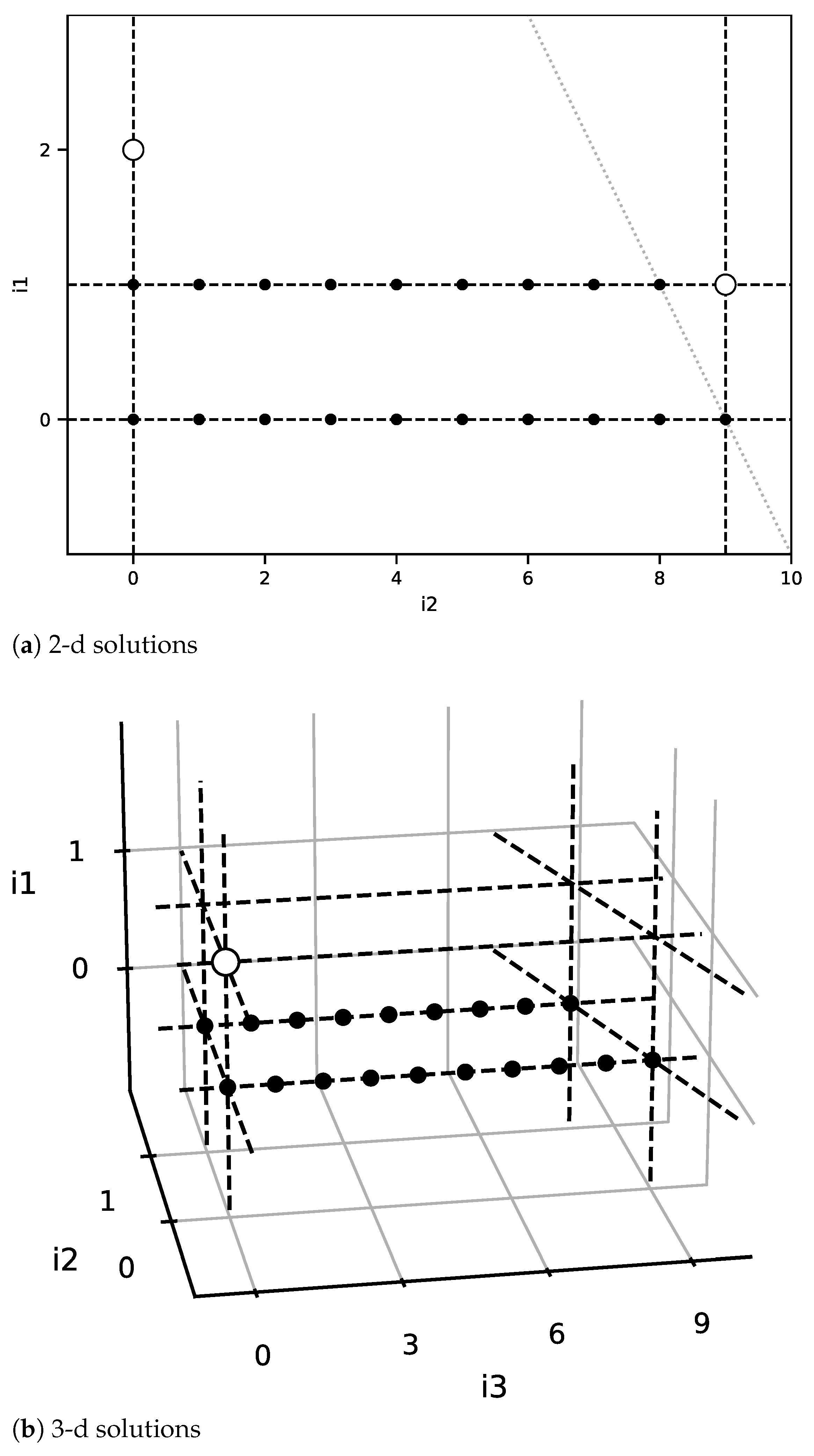
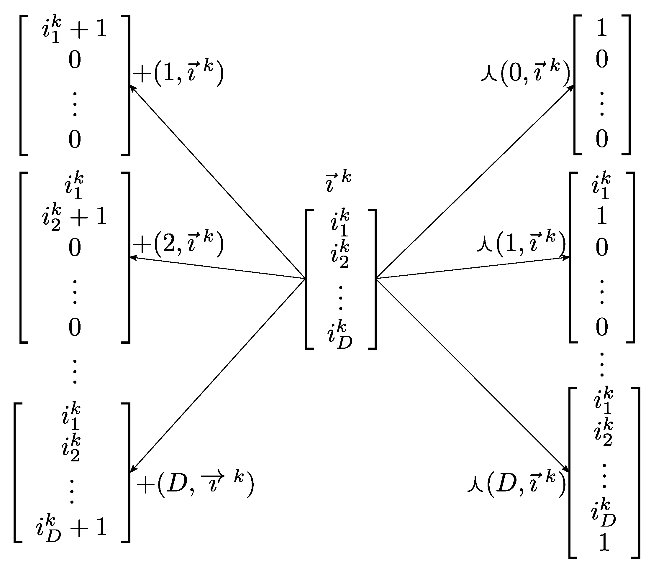
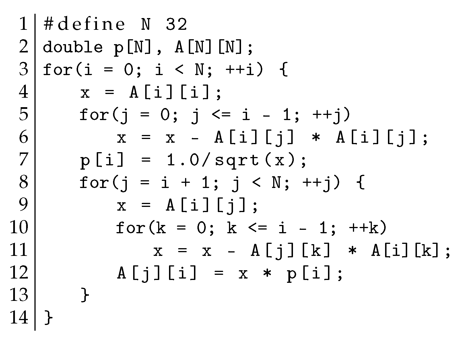
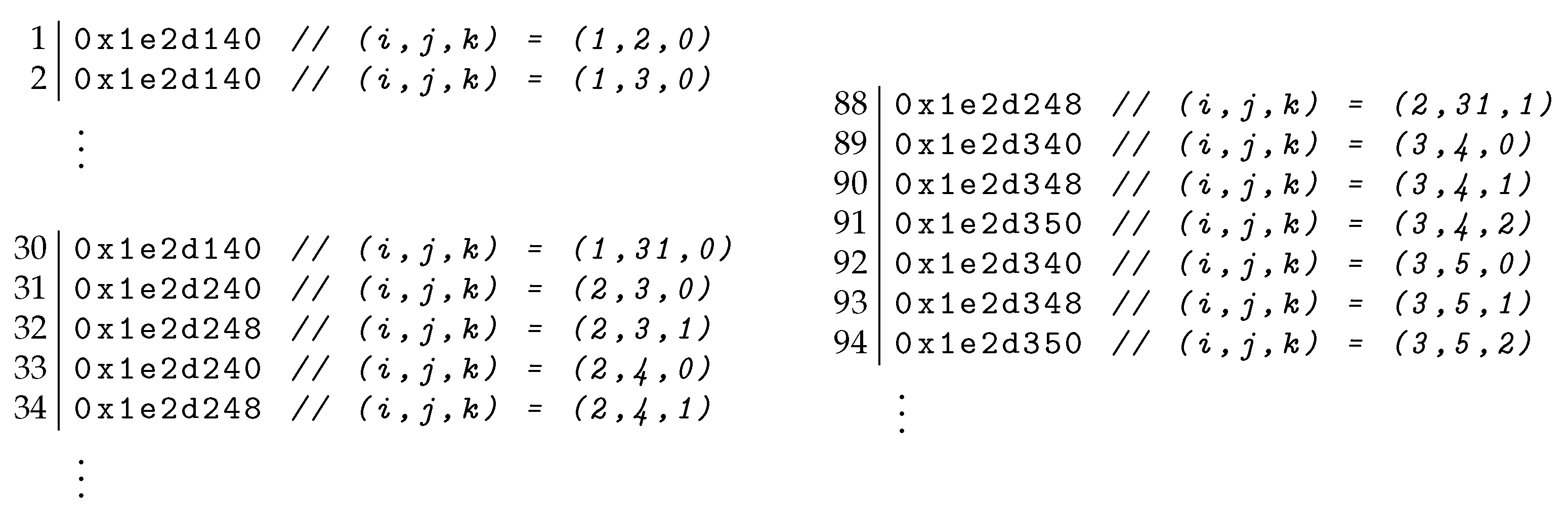
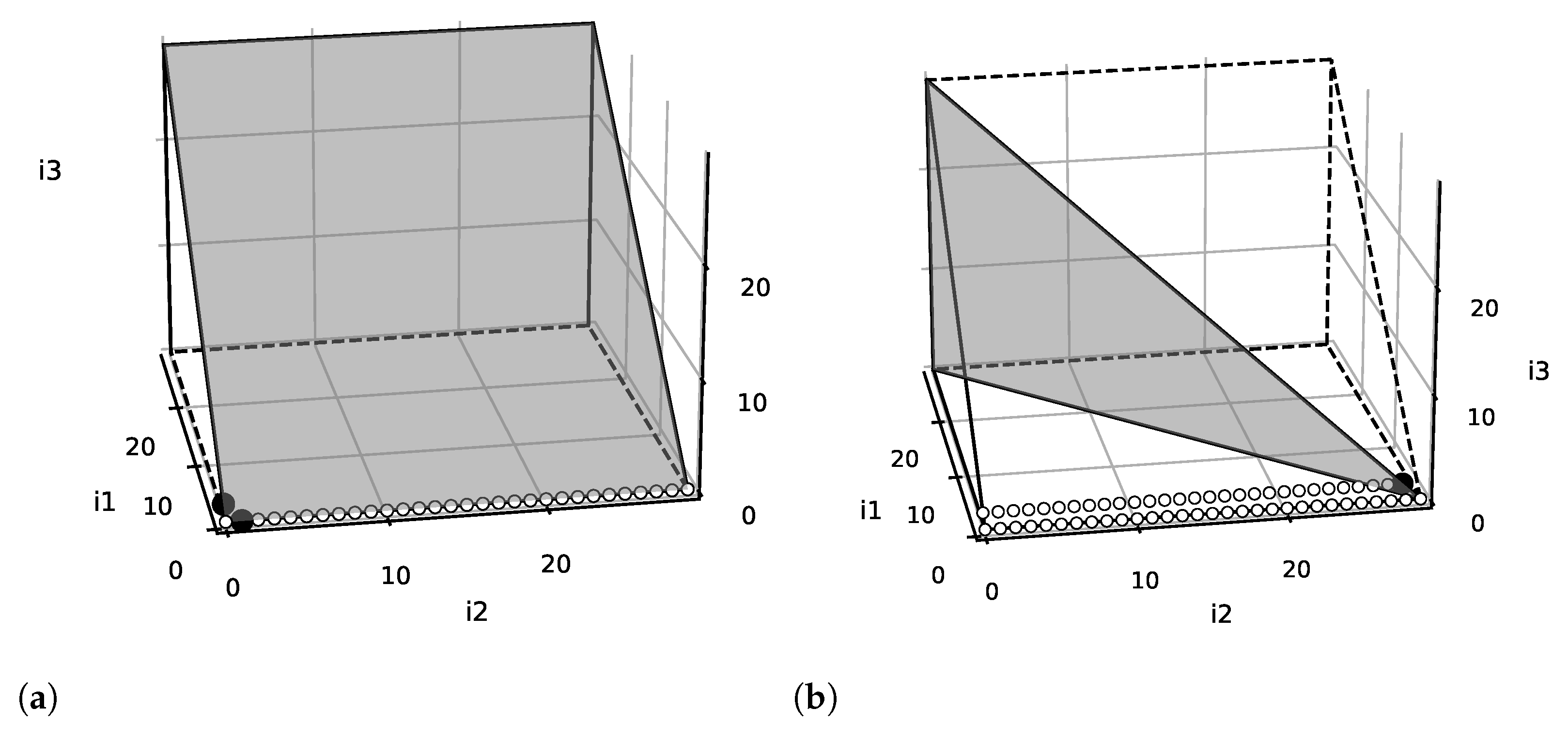
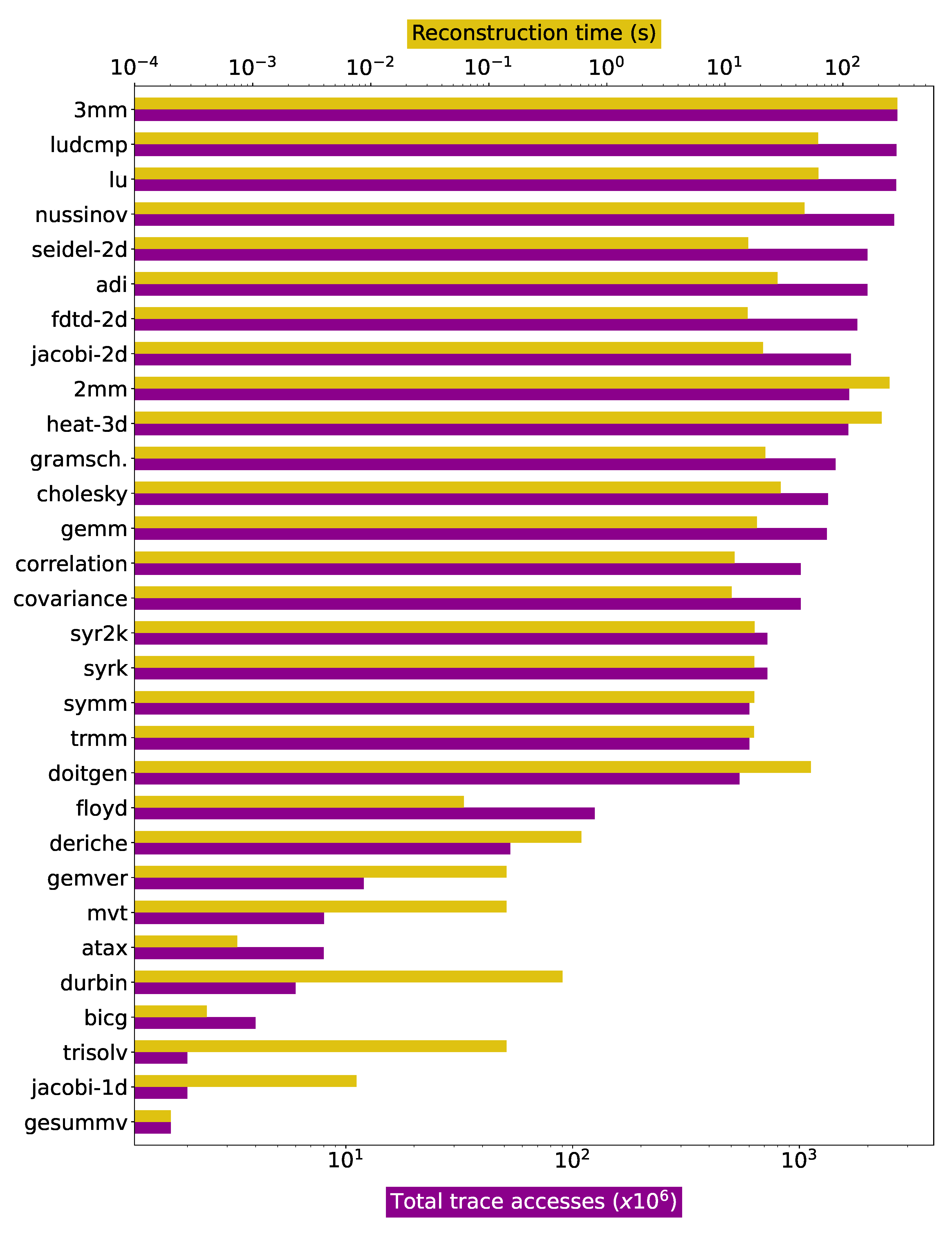
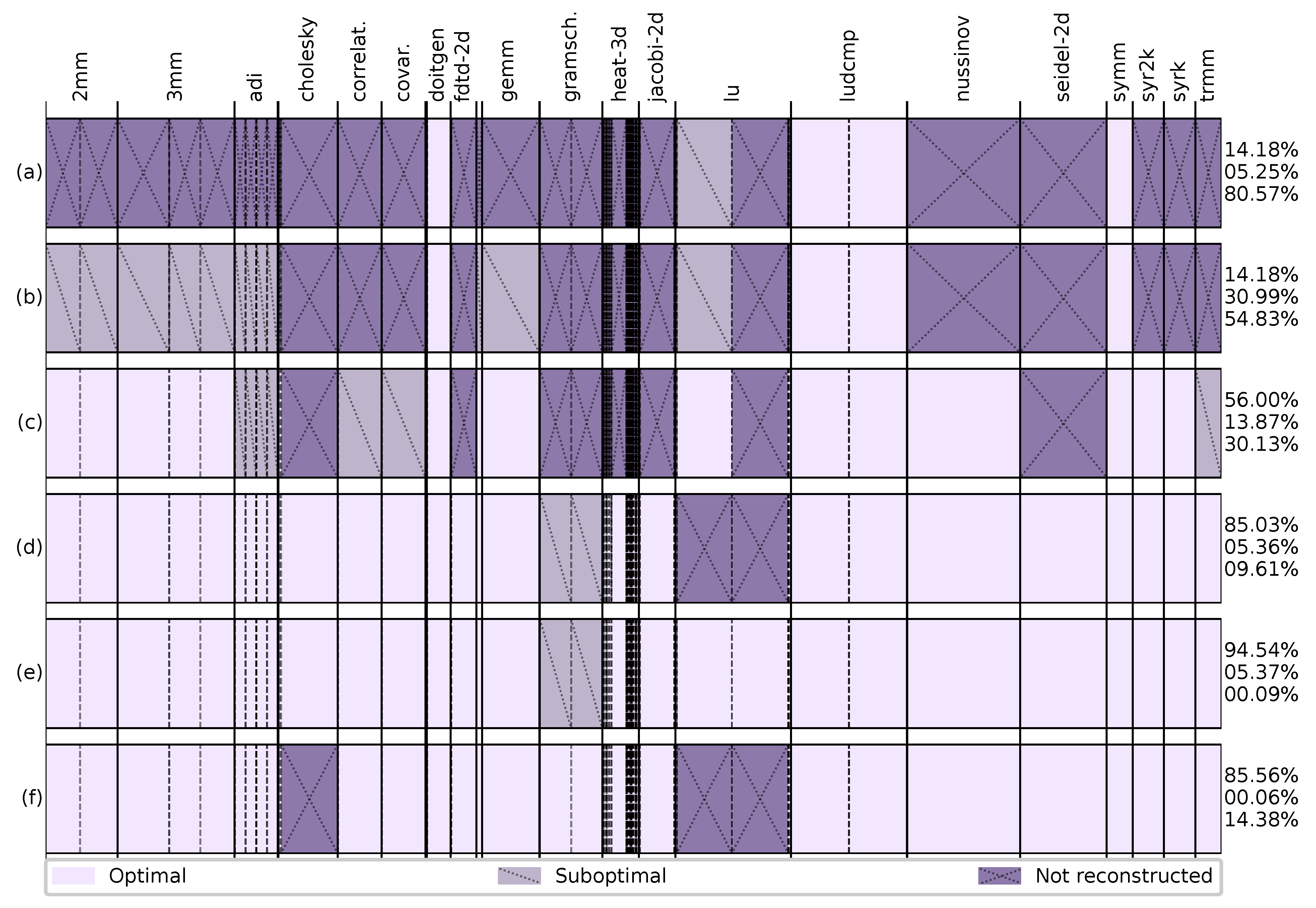
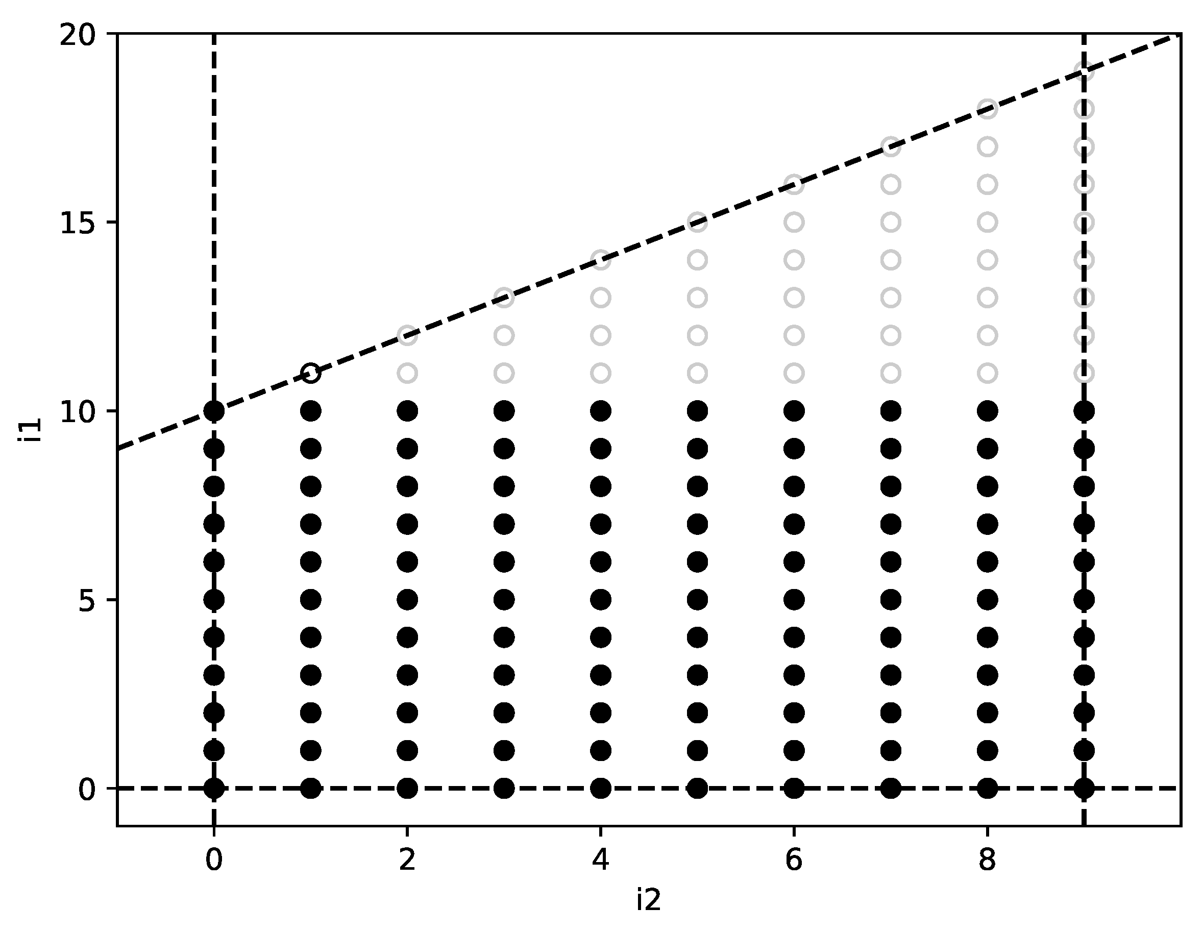
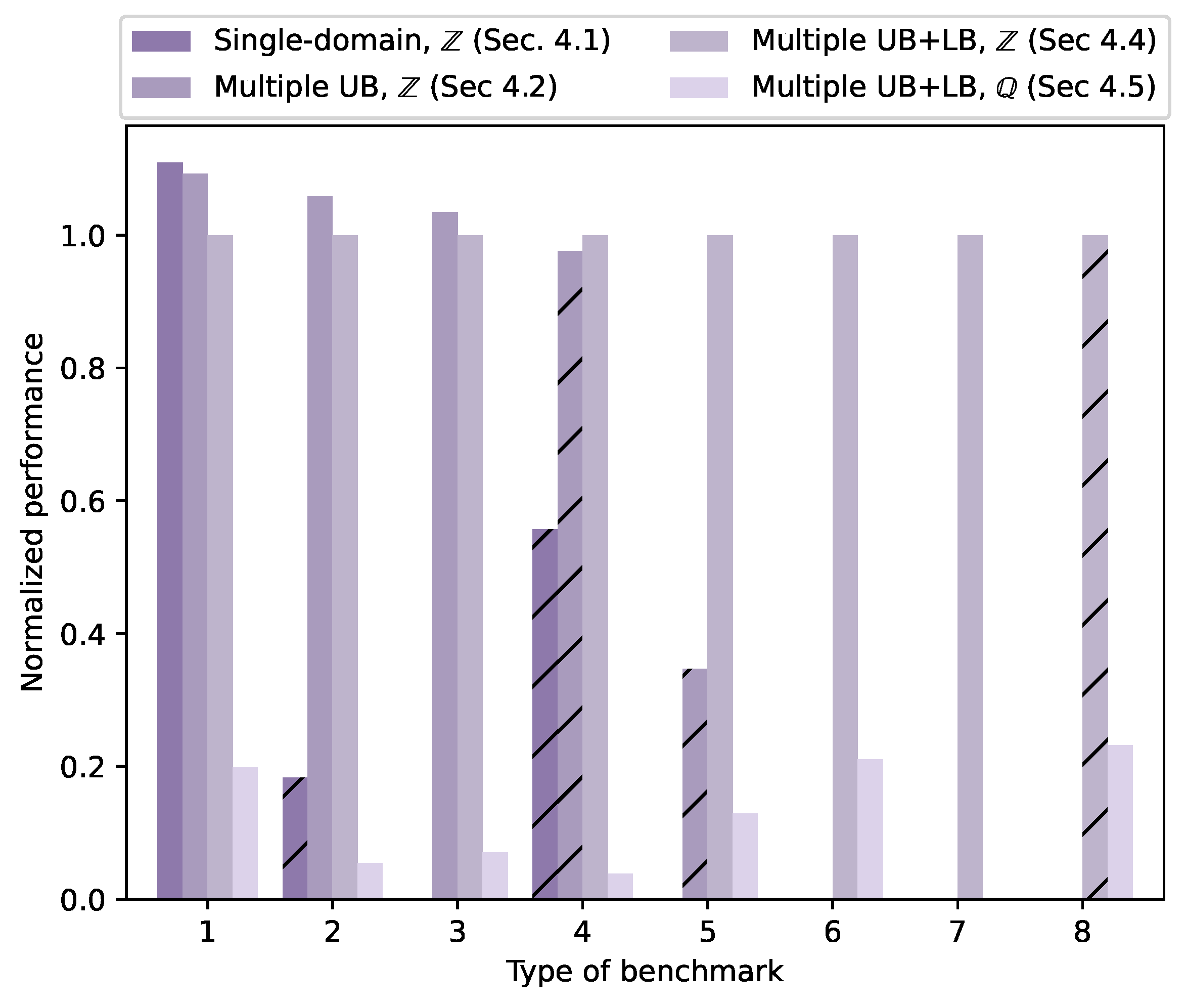
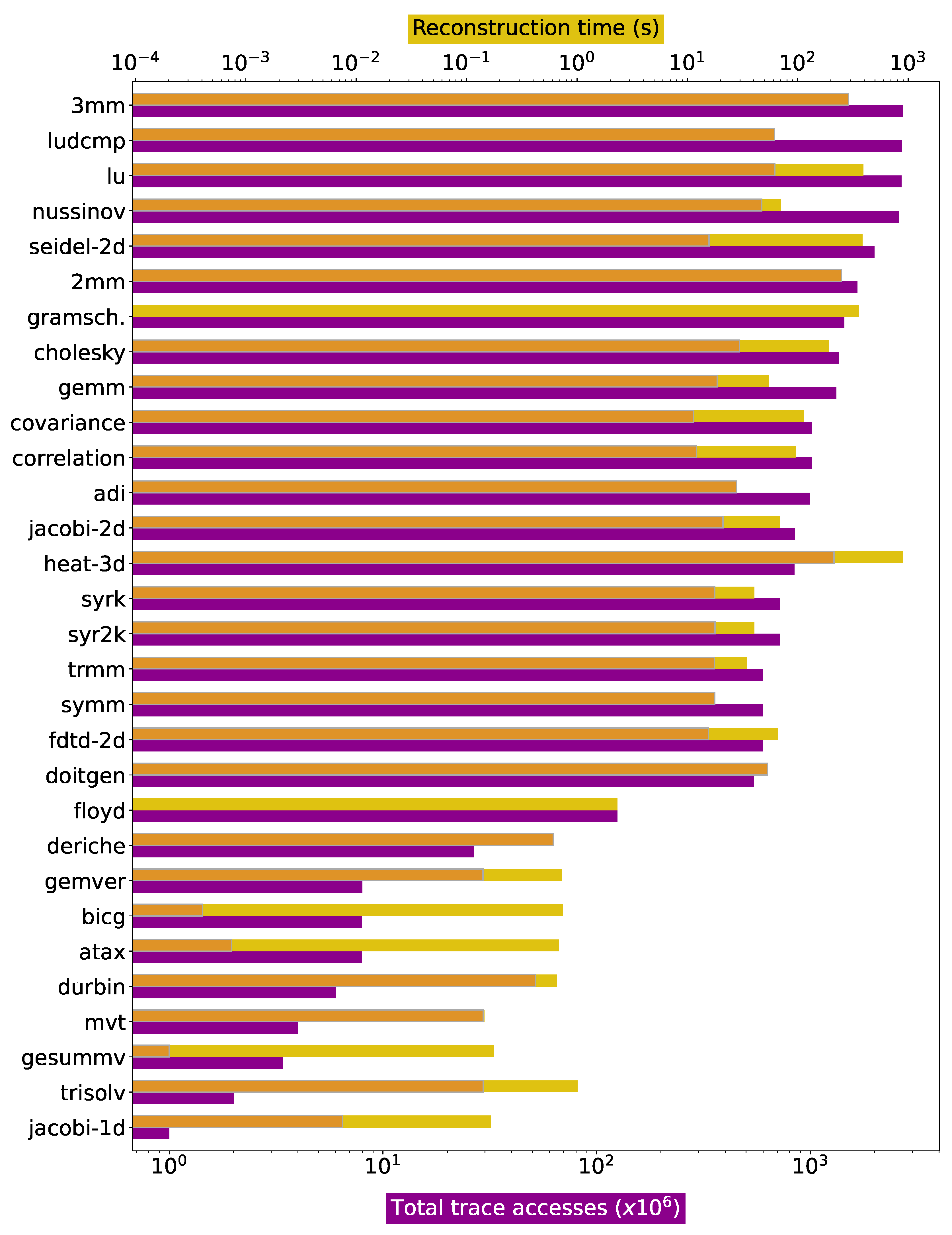
Table 1.
Characteristics of the PolyBench/C benchmarks. The number of loop scopes, trace size and maximum loop depth are shown for both original and Pluto-tiled versions of each code. The “Type” column in the “Tiled” part shows the details of the benchmark grouping addressed in Section 4.6.
Table 1.
Characteristics of the PolyBench/C benchmarks. The number of loop scopes, trace size and maximum loop depth are shown for both original and Pluto-tiled versions of each code. The “Type” column in the “Tiled” part shows the details of the benchmark grouping addressed in Section 4.6.
| Benchmark | Original (Section 3.6) | Tiled (Section 4.6) | |||||
|---|---|---|---|---|---|---|---|
| #Scopes | #Accesses () | Max. Depth | #Scopes | #Accesses () | Max. Depth | Type | |
| 2 mm | 4 | 1657.58 | 2 | 6 | 1656.96 | 6 | 2 |
| 3 mm | 6 | 2702.59 | 3 | 6 | 2701.71 | 6 | 2 |
| adi | 6 | 1993.01 | 3 | 12 | 996.00 | 5 | 4 |
| atax | 4 | 7.98 | 1 | 4 | 7.984 | 4 | 2 |
| bicg | 3 | 3.99 | 1 | 4 | 7.984 | 4 | 2 |
| cholesky | 4 | 1335.33 | 3 | 10 | 1363.90 | 6 | 7 |
| correlation | 8 | 1012.92 | 3 | 9 | 1013.64 | 6 | 3 |
| covariance | 5 | 1012.92 | 3 | 7 | 1013.64 | 6 | 3 |
| deriche | 6 | 53.08 | 2 | 3 | 26.54 | 4 | 2 |
| doitgen | 3 | 544.32 | 3 | 3 | 544.32 | 4 | 1 |
| durbin | 4 | 6.00 | 2 | 4 | 6.00 | 2 | 1 |
| fdtd-2d | 4 | 1798.40 | 3 | 7 | 598.93 | 6 | 6 |
| floyd-warshall | 1 | 125.00 | 2 | 1 | 125.00 | 5 | 2 |
| gemm | 2 | 1321.10 | 3 | 2 | 1321.10 | 6 | 2 |
| gemver | 4 | 12.00 | 2 | 3 | 8.00 | 4 | 2 |
| gesummv | 2 | 1.69 | 1 | 5 | 3.38 | 4 | 2 |
| gramschmidt | 6 | 1441.92 | 3 | 5 | 1441.92 | 5 | 8 |
| heat-3d | 2 | 1643.03 | 4 | 86 | 842.23 | 8 | 7 |
| jacobi-1d | 2 | 2.00 | 2 | 6 | 1.00 | 4 | 3 |
| jacobi-2d | 2 | 1684.80 | 3 | 23 | 843.70 | 6 | 6 |
| lu | 3 | 2666.67 | 3 | 13 | 2666.67 | 6 | 7 |
| ludcmp | 8 | 2672.67 | 3 | 15 | 2676.66 | 3 | 1 |
| mvt | 2 | 8.00 | 2 | 1 | 4.00 | 4 | 2 |
| nussinov | 5 | 2610.41 | 3 | 6 | 2604.17 | 5 | 5 |
| seidel-2d | 1 | 1996.00 | 3 | 1 | 1996.00 | 6 | 6 |
| symm | 2 | 600.60 | 3 | 5 | 600.60 | 3 | 1 |
| syr2k | 2 | 721.32 | 3 | 2 | 721.32 | 6 | 3 |
| syrk | 2 | 721.32 | 3 | 2 | 721.32 | 6 | 3 |
| trisolv | 2 | 2.00 | 2 | 5 | 2.00 | 4 | 2 |
| trmm | 2 | 600.60 | 3 | 2 | 600.60 | 6 | 3 |
Table 2.
Benchmark types used in Figure 10 according to reconstruction strategy coverage. The symbols, ✓, ∼, and × indicate optimal, suboptimal (excess dimensionality), and failed reconstruction, respectively.
Table 2.
Benchmark types used in Figure 10 according to reconstruction strategy coverage. The symbols, ✓, ∼, and × indicate optimal, suboptimal (excess dimensionality), and failed reconstruction, respectively.
| Type | Single | Mult. UB | Mult. UB+LB | Mult. UB+LB |
|---|---|---|---|---|
| 1 | ✓ | ✓ | ✓ | ✓ |
| 2 | ∼ | ✓ | ✓ | ✓ |
| 3 | × | ✓ | ✓ | ✓ |
| 4 | ∼ | ∼ | ✓ | ✓ |
| 5 | × | ∼ | ✓ | ✓ |
| 6 | × | × | ✓ | ✓ |
| 7 | × | × | ✓ | × |
| 8 | × | × | ∼ | ✓ |
Publisher’s Note: MDPI stays neutral with regard to jurisdictional claims in published maps and institutional affiliations. |
© 2021 by the authors. Licensee MDPI, Basel, Switzerland. This article is an open access article distributed under the terms and conditions of the Creative Commons Attribution (CC BY) license (https://creativecommons.org/licenses/by/4.0/).
Share and Cite
MDPI and ACS Style
Rodríguez, G.; Pouchet, L.-N.; Touriño, J. Representing Integer Sequences Using Piecewise-Affine Loops. Mathematics 2021, 9, 2368. https://0-doi-org.brum.beds.ac.uk/10.3390/math9192368
AMA Style
Rodríguez G, Pouchet L-N, Touriño J. Representing Integer Sequences Using Piecewise-Affine Loops. Mathematics. 2021; 9(19):2368. https://0-doi-org.brum.beds.ac.uk/10.3390/math9192368
Chicago/Turabian StyleRodríguez, Gabriel, Louis-Noël Pouchet, and Juan Touriño. 2021. "Representing Integer Sequences Using Piecewise-Affine Loops" Mathematics 9, no. 19: 2368. https://0-doi-org.brum.beds.ac.uk/10.3390/math9192368
Note that from the first issue of 2016, this journal uses article numbers instead of page numbers. See further details here.