
Non-Sequential Linear Construction Project Scheduling Model for Minimizing Idle Equipment Using Constraint Programming (CP)


Abstract
:1. Introduction
1.1. Background
1.2. Objectives
1.3. Paper Structure
2. Literature Review
3. Materials and Methods
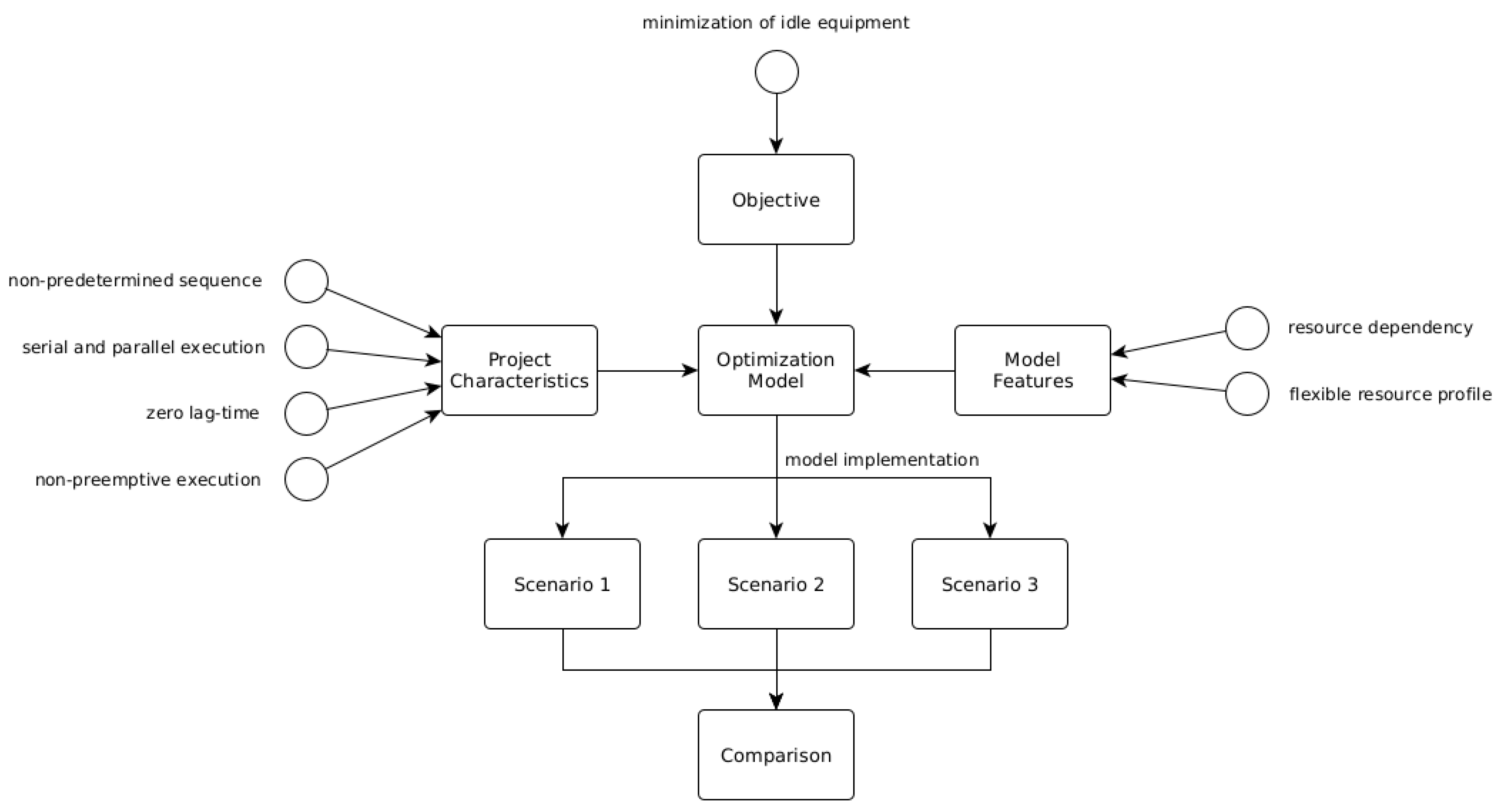
3.1. Model Concept
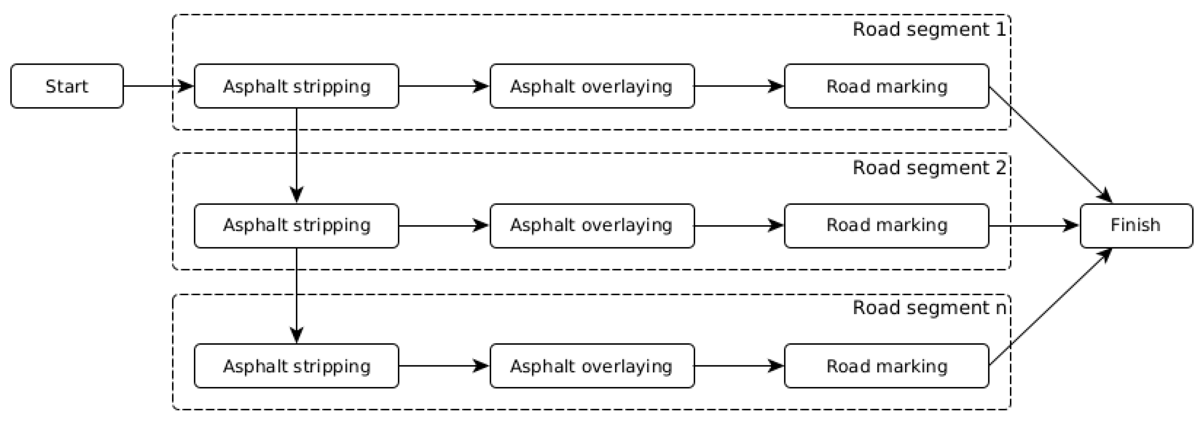
3.1.1. Project Characteristics
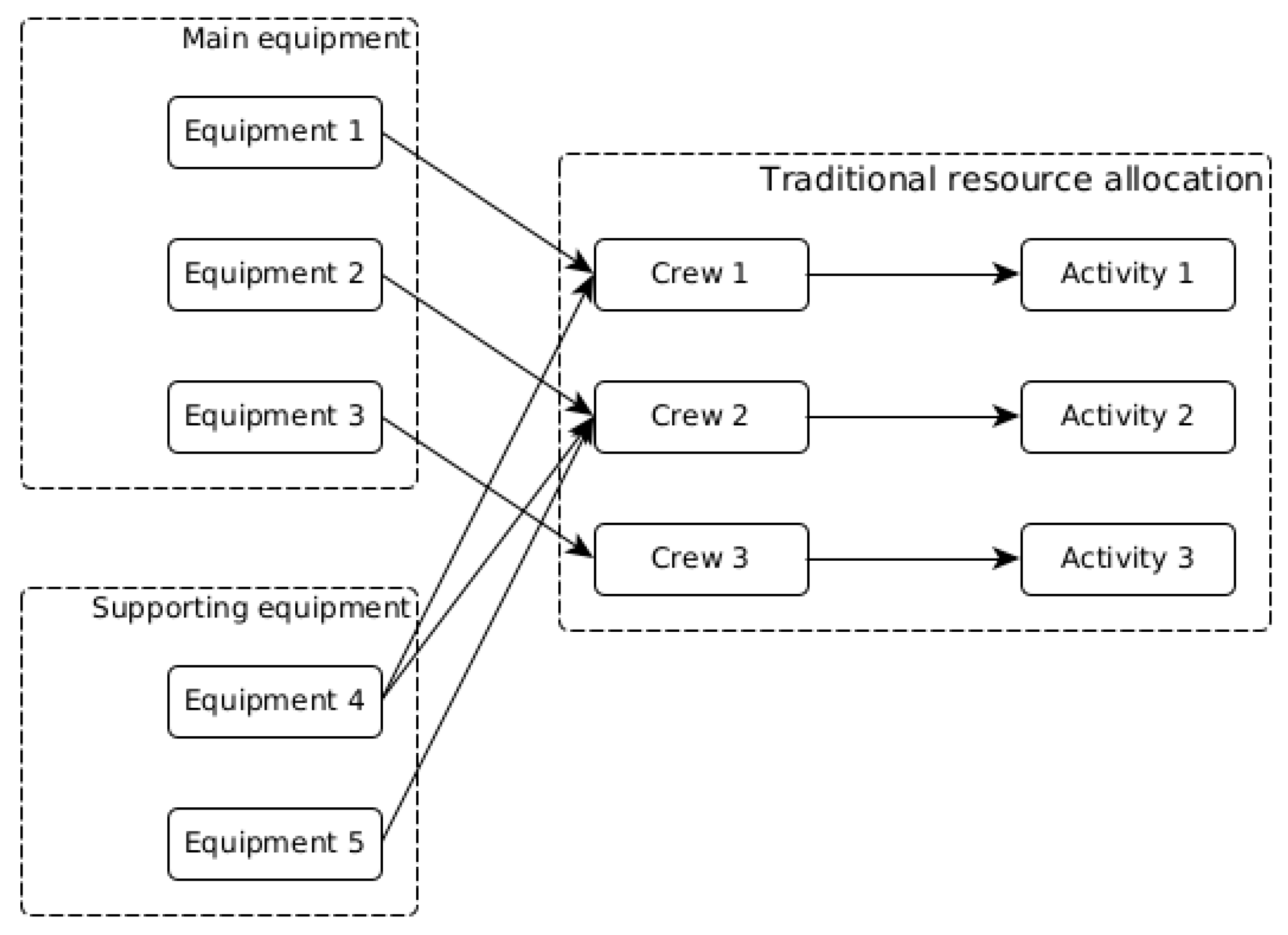
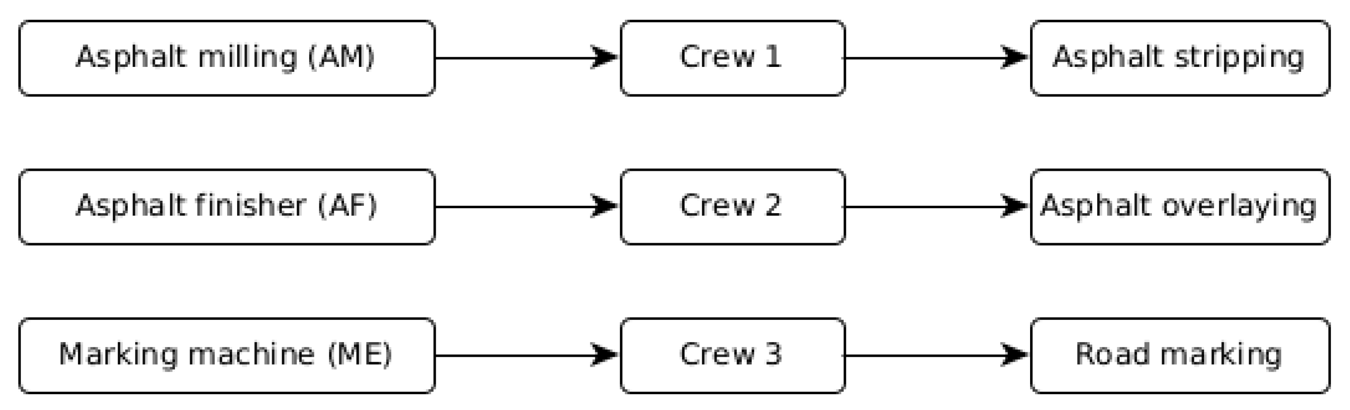
3.1.2. Equipment Combination and Configuration (ECC)
3.1.3. Model Features
3.1.4. Model Objective
3.2. Model Formulation
3.2.1. Input Data
3.2.2. Decision Variables
3.2.3. Decision Expressions
3.2.4. Objective Function
3.2.5. Constraints
3.2.6. Model Implementation Scenario
4. Result and Discussion
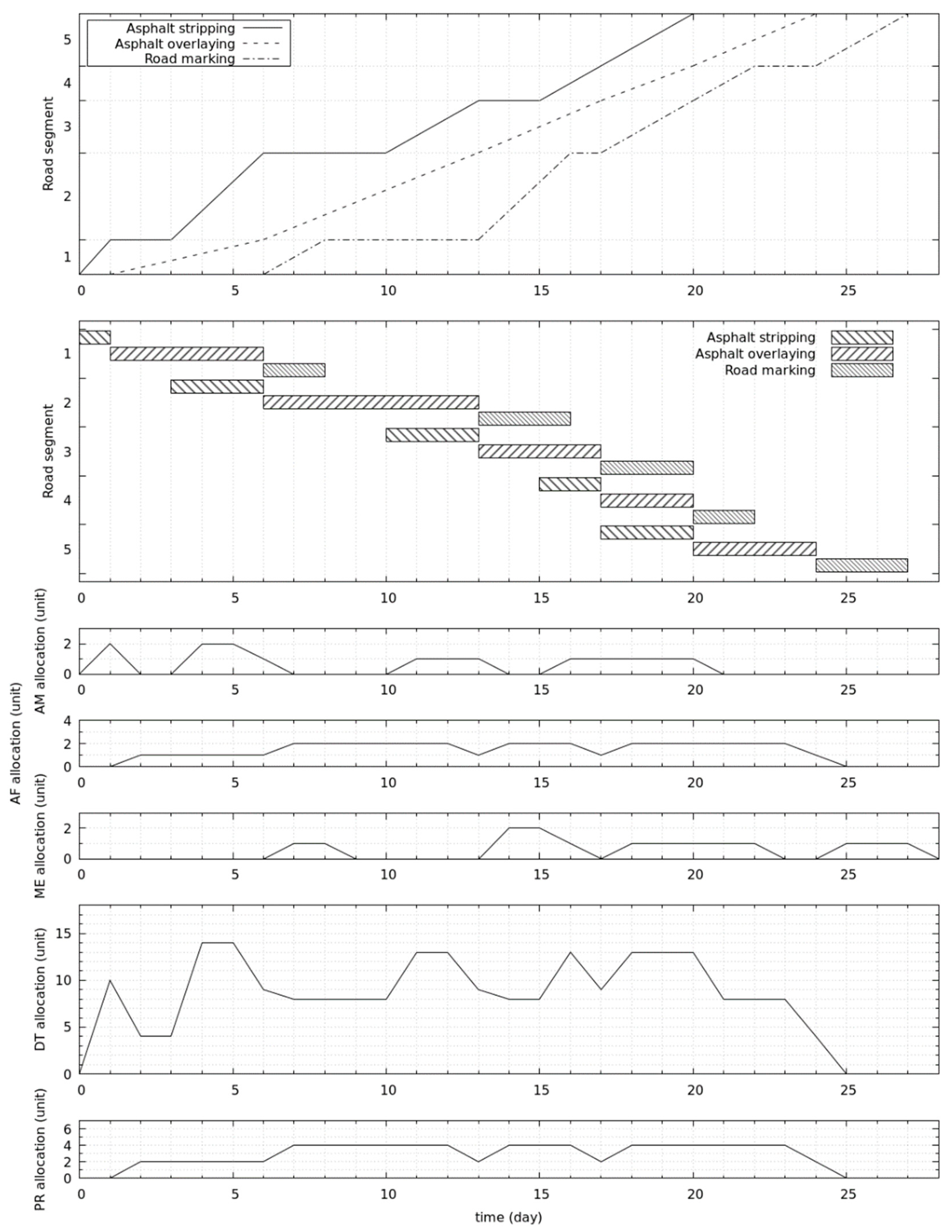
4.1. Scenario 1: Traditional LSM
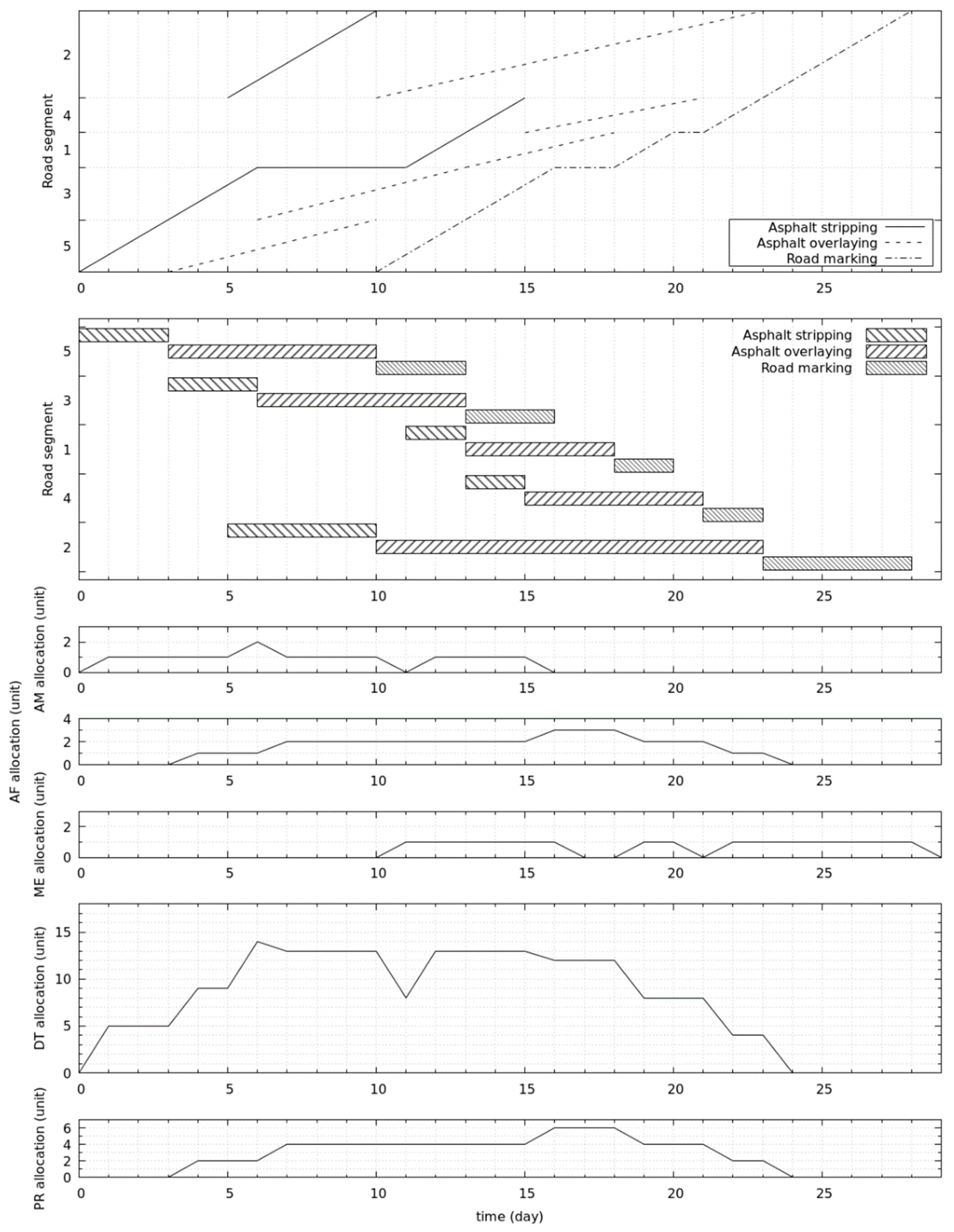
4.2. Scenario 2: Proposed Model with the Rectangular Resource Profile
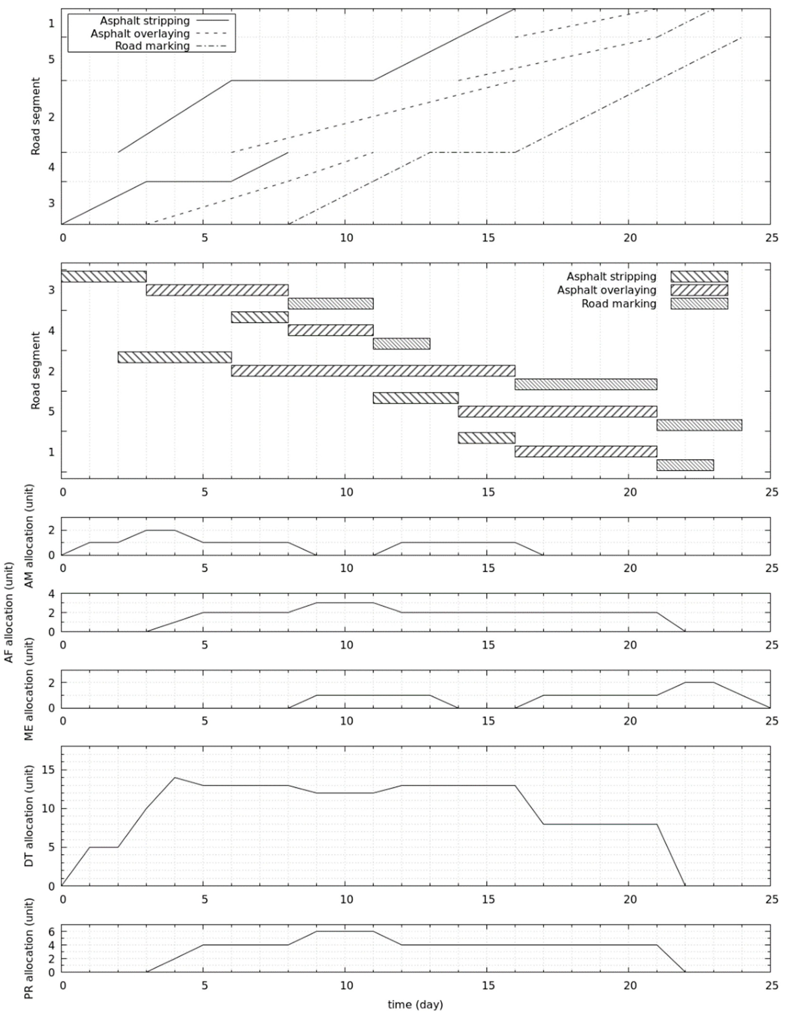
4.3. Scenario 3: Proposed Model with the Flexible Resource Profile
4.4. Comparison
5. Conclusions
Author Contributions
Funding
Institutional Review Board Statement
Informed Consent Statement
Data Availability Statement
Conflicts of Interest
References
- Pinedo, M.L. Scheduling: Theory, Algorithms, and Systems, 4th ed.; Springer: New York, NY, USA, 2012; Volume 4. [Google Scholar]
- Damci, A.; Arditi, D.; Polat, G. Multiresource leveling in line-of-balance scheduling. J. Constr. Eng. Manag. 2013, 139, 1108–1116. [Google Scholar] [CrossRef]
- Tao, S.; Wu, C.; Sheng, Z.; Wang, X. Space-time repetitive project scheduling considering location and congestion. J. Comput. Civ. Eng. 2018, 32. [Google Scholar] [CrossRef]
- Wu, C.; Wang, X.; Lin, J. Optimizations in project scheduling: A state-of-art survey. In Optimization and Control Methods in Industrial Engineering and Construction; Springer: Berlin/Heidelberg, Germany, 2014; pp. 161–177. [Google Scholar]
- Hyari, K.; El-Rayes, K. Optimal planning and scheduling for repetitive construction projects. J. Manag. Eng. 2006, 22, 11–19. [Google Scholar] [CrossRef]
- Zhang, L.; Dai, G.; Zou, X.; Qi, J. Robustness-based multi-objective optimization for repetitive projects under work continuity uncertainty. Eng. Constr. Archit. Manag. 2020. [Google Scholar] [CrossRef]
- Esfahan, N.R.; Razavi, S. Uncertainty-aware linear schedule optimization: A space-time constraint-satisfaction approach. J. Constr. Eng. Manag. 2017, 143. [Google Scholar] [CrossRef]
- Moselhi, O.; Hassanein, A. Optimized scheduling of linear projects. J. Constr. Eng. Manag. 2003, 129, 664–673. [Google Scholar] [CrossRef]
- Adeli, H.; Karim, A. Construction Scheduling, Cost Optimization and Management; CRC Press: Boca Raton, FL, USA, 2001; ISBN 0429076770. [Google Scholar]
- Bakry, I.; Moselhi, O.; Zayed, T. Optimized acceleration of repetitive construction projects. Autom. Constr. 2014, 39, 145–151. [Google Scholar] [CrossRef]
- Ipsilandis, P.G. Multiobjective linear programming model for scheduling linear repetitive projects. J. Constr. Eng. Manag. 2007, 133, 417–424. [Google Scholar] [CrossRef]
- Roghabadi, M.A.; Moselhi, O. Optimized crew selection for scheduling of repetitive projects. Eng. Constr. Archit. Manag. 2020, 28, 1517–1540. [Google Scholar] [CrossRef]
- Brucker, P.; Drexl, A.; Möhring, R.; Neumann, K.; Pesch, E. Resource-constrained project scheduling: Notation, classification, models, and methods. Eur. J. Oper. Res. 1999, 112, 3–41. [Google Scholar] [CrossRef]
- Lucko, G.; Araújo, L.G.; Cates, G.R. Slip chart–inspired project schedule diagramming: Origins, buffers, and extension to linear schedules. J. Constr. Eng. Manag. 2016, 142, 4015101. [Google Scholar] [CrossRef]
- Liu, S.S.; Budiwirawan, A.; Arifin, M.F.A.; Chen, W.T.; Huang, Y.H. Optimization model for the pavement pothole repair problem considering consumable resources. Symmetry 2021, 13, 364. [Google Scholar] [CrossRef]
- Katsuragawa, C.M.; Lucko, G.; Isaac, S.; Su, Y. Fuzzy linear and repetitive scheduling for construction projects. J. Constr. Eng. Manag. 2021, 147. [Google Scholar] [CrossRef]
- Su, Y.; Lucko, G. Linear scheduling with multiple crews based on line-of-balance and productivity scheduling method with singularity functions. Autom. Constr. 2016, 70, 38–50. [Google Scholar] [CrossRef]
- Lucko, G.; Gattei, G. Line-of-balance against linear scheduling: Critical comparison. Proc. Inst. Civ. Eng. Manag. Procure. Law 2016, 169, 26–44. [Google Scholar] [CrossRef]
- Tang, Y.; Liu, R.; Sun, Q. Two-stage scheduling model for resource leveling of linear projects. J. Constr. Eng. Manag. 2014, 140, 4014022. [Google Scholar] [CrossRef]
- Harmelink, D.J.; Rowings, J. Linear scheduling model: Development of controlling activity path. J. Constr. Eng. Manag. 1998, 124, 263–268. [Google Scholar] [CrossRef]
- Roofigari-Esfahan, N.; Paez, A.; N. Razavi, S. Location-aware scheduling and control of linear projects: Introducing space-time float prisms. J. Constr. Eng. Manag. 2015, 141, 06014008. [Google Scholar] [CrossRef]
- Duffy, G.A.; Oberlender, G.D.; Seok Jeong, D.H. Linear scheduling model with varying production rates. J. Constr. Eng. Manag. 2011, 137, 574–582. [Google Scholar] [CrossRef] [Green Version]
- Harmelink, D.J. Linear scheduling model: Float characteristics. J. Constr. Eng. Manag. 2001, 127, 255–260. [Google Scholar] [CrossRef]
- Mattila, K.; Abraham, D. Resource leveling of linear schedules using integer linear programming. J. Constr. Eng. Manag. 1998, 124, 232–244. [Google Scholar] [CrossRef]
- El-Rayes, K.; Jun, D.H. Optimizing resource leveling in construction projects. J. Constr. Eng. Manag. 2009, 135, 1172–1180. [Google Scholar] [CrossRef]
- Mizutani, D.; Nakazato, Y.; Lee, J. Network-level synchronized pavement repair and work zone policies: Optimal solution and rule-based approximation. Transp. Res. Part C Emerg. Technol. 2020, 120, 102797. [Google Scholar] [CrossRef]
- Huang, S.-H.; Lin, P.-C. Multi-treatment capacitated arc routing of construction machinery in Taiwan’s smooth road project. Autom. Constr. 2012, 21, 210–218. [Google Scholar] [CrossRef]
- Aarabi, F.; Batta, R. Scheduling spatially distributed jobs with degradation: Application to pothole repair. Socioecon. Plann. Sci. 2020, 72, 100904. [Google Scholar] [CrossRef]
- Georgy, M.E. Evolutionary resource scheduler for linear projects. Autom. Constr. 2008, 17, 573–583. [Google Scholar] [CrossRef]
- Tang, Y.; Liu, R.; Wang, F.; Sun, Q.; Kandil, A.A. Scheduling optimization of linear schedule with constraint programming. Comput. Civ. Infrastruct. Eng. 2018, 33, 124–151. [Google Scholar] [CrossRef]
- Hojjat, A.; Samanwoy, G.-D. Mesoscopic-wavelet freeway work zone flow and congestion feature extraction model. J. Transp. Eng. 2004, 130, 94–103. [Google Scholar] [CrossRef]
- Adeli, H.; Karim, A. Scheduling/cost optimization and neural dynamics model for construction. J. Constr. Eng. Manag. 1997, 123, 450–458. [Google Scholar] [CrossRef]
- Xiaomo, J.; Hojjat, A. Freeway work zone traffic delay and cost optimization model. J. Transp. Eng. 2003, 129, 230–241. [Google Scholar] [CrossRef]
- Shayanfar, E.; Schonfeld, P. Selecting and scheduling interrelated road projects with uncertain demand. Transp. A Transp. Sci. 2019, 15, 1712–1733. [Google Scholar] [CrossRef]
- Koulinas, G.K.; Anagnostopoulos, K.P. Construction resource allocation and leveling using a threshold accepting–based hyperheuristic algorithm. J. Constr. Eng. Manag. 2012, 138, 854–863. [Google Scholar] [CrossRef]
- Hegazy, T. Optimization of resource allocation and leveling using genetic algorithms. J. Constr. Eng. Manag. 1999, 125, 167–175. [Google Scholar] [CrossRef]
- Moselhi, O.; Lorterapong, P. least impact algorithm for resource allocation. Can. J. Civ. Eng. 1993, 20, 180–188. [Google Scholar] [CrossRef]
- Tang, Y.; Liu, R.; Sun, Q. Schedule control model for linear projects based on linear scheduling method and constraint programming. Autom. Constr. 2014, 37, 22–37. [Google Scholar] [CrossRef]
- Lucko, G. Integrating efficient resource optimization and linear schedule analysis with singularity functions. J. Constr. Eng. Manag. 2011, 137, 45–55. [Google Scholar] [CrossRef]
- Wang, Z.; Hu, Z.; Tang, Y. Float-based resource leveling optimization of linear projects. IEEE Access 2020, 8, 176997–177020. [Google Scholar] [CrossRef]
- Heon Jun, D.; El-Rayes, K. Multiobjective optimization of resource leveling and allocation during construction scheduling. J. Constr. Eng. Manag. 2011, 137, 1080–1088. [Google Scholar] [CrossRef]
- Fündeling, C.-U.; Trautmann, N. A Priority-rule method for project scheduling with work-content constraints. Eur. J. Oper. Res. 2010, 203, 568–574. [Google Scholar] [CrossRef]
- Naber, A.; Kolisch, R. MIP Models for resource-constrained project scheduling with flexible resource profiles. Eur. J. Oper. Res. 2014, 239, 335–348. [Google Scholar] [CrossRef]
- Leu, S.-S.; Hwang, S.-T. Optimal repetitive scheduling model with shareable resource constraint. J. Constr. Eng. Manag. 2001, 127, 270–280. [Google Scholar] [CrossRef]
- Liu, S.S.; Wang, C.J. Optimization model for resource assignment problems of linear construction projects. Autom. Constr. 2007, 16, 460–473. [Google Scholar] [CrossRef]
- Zhang, L.; Zou, X.; Kan, Z. Improved strategy for resource allocation in repetitive projects considering the learning effect. J. Constr. Eng. Manag. 2014, 140, 4014053. [Google Scholar] [CrossRef]
- Kong, F.; Dou, D. Resource-constrained project scheduling problem under multiple time constraints. J. Constr. Eng. Manag. 2021, 147. [Google Scholar] [CrossRef]
- Siu, M.-F.F.; Lu, M.; AbouRizk, S. Resource supply-demand matching scheduling approach for construction workface planning. J. Constr. Eng. Manag. 2016, 142, 4015048. [Google Scholar] [CrossRef]
- Khanzadi, M.; Kaveh, A.; Alipour, M.; Aghmiuni, H.K. Application of CBO and CSS for resource allocation and resource leveling problem. Iran. J. Sci. Technol. Trans. Civ. Eng. 2016, 40, 1–10. [Google Scholar] [CrossRef]
- Tang, Y.; Sun, Q.; Liu, R.; Wang, F. Resource leveling based on line of balance and constraint programming. Comput. Civ. Infrastruct. Eng. 2018, 33, 864–884. [Google Scholar] [CrossRef]
- Bendoly, E.; Perry-Smith, J.E.; Bachrach, D.G. The perception of difficulty in project-work planning and its impact on resource sharing. J. Oper. Manag. 2010, 28, 385–397. [Google Scholar] [CrossRef]
- Xu, J.; Meng, J.; Zeng, Z.; Wu, S.; Shen, M. Resource sharing-based multiobjective multistage construction equipment allocation under fuzzy environment. J. Constr. Eng. Manag. 2013, 139, 161–173. [Google Scholar] [CrossRef]


| Research | Objective | Resource | Activity Duration | Method |
|---|---|---|---|---|
| [2] | Resource leveling | Multiple types of resource. | Production rate and duration are based on the resource which requires longest time. | Genetic algorithm (GA) |
| [44] | Multi objective (production duration, resource amount, minimum makespan) | Multiple types of resources. | Activity duration is based resource allocation. | Genetic algorithm (GA) |
| [38] | Resource leveling | The type resource is implicitly represented by the type of work. | Duration is based on resource’s production rate. | Constraint programming (CP) |
| [40] | Resource leveling | Multiple types of resources used by an activity. | Duration is based on resource’s production rate. | Quantum-behaved particle swarm optimization (QPSO) |
| [50] | Resource leveling | The type resource is implicitly represented by the type of work. | Duration is based on resource’s production rate. | Constraint programming (CP) |
| Proposed model | Resource idleness minimization | Multiple types of resources used by an activity. | Activity duration is based resource allocation and equipment combination and configuration (ECC). | Constraint programming (CP) |
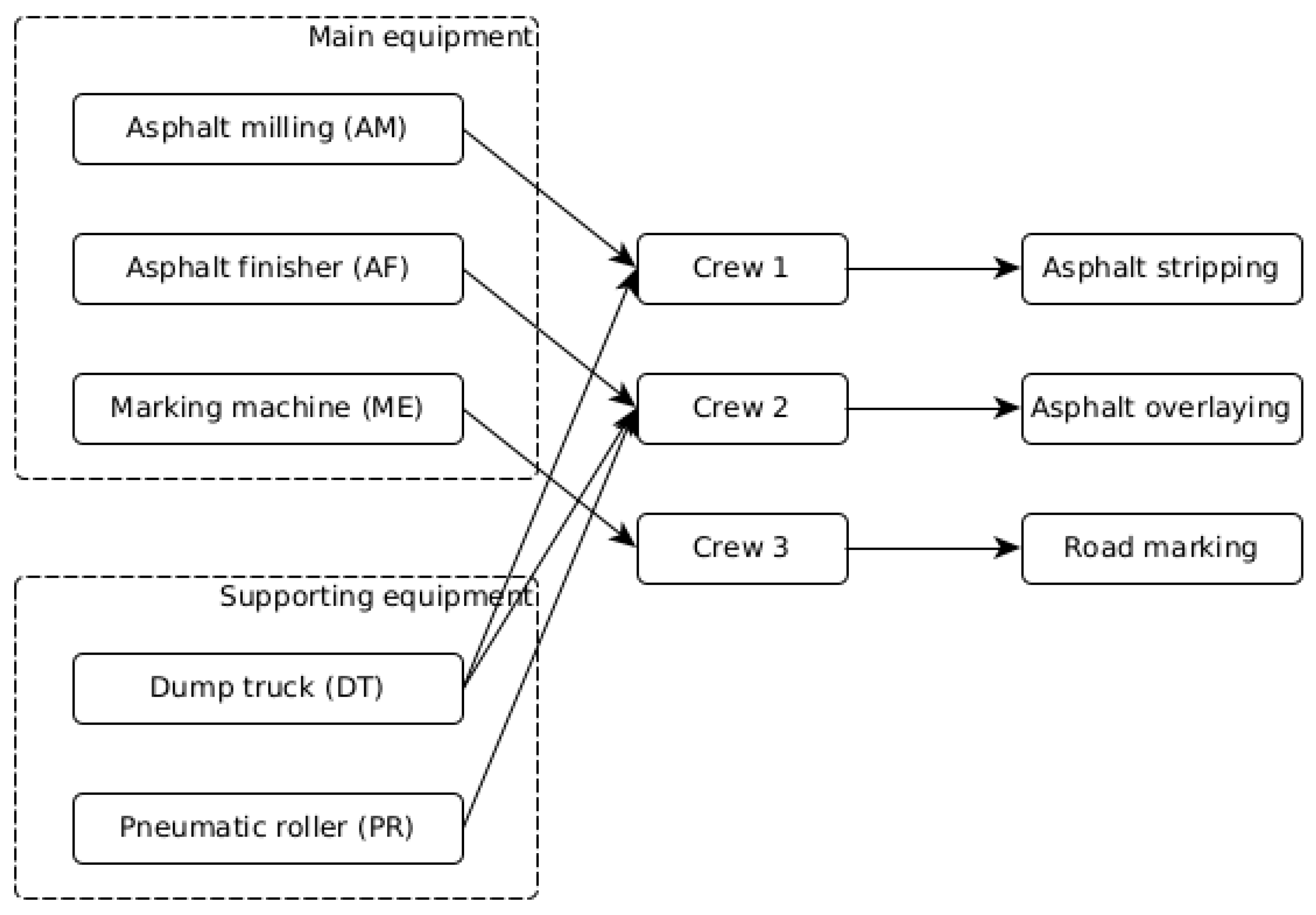
| Activity Name | Main Equipment |
|---|---|
| Asphalt stripping | Asphalt milling machine (AM) |
| Asphalt resurfacing | Asphalt finisher machine (AF) |
| Road marking | Road marking machine (ME) |
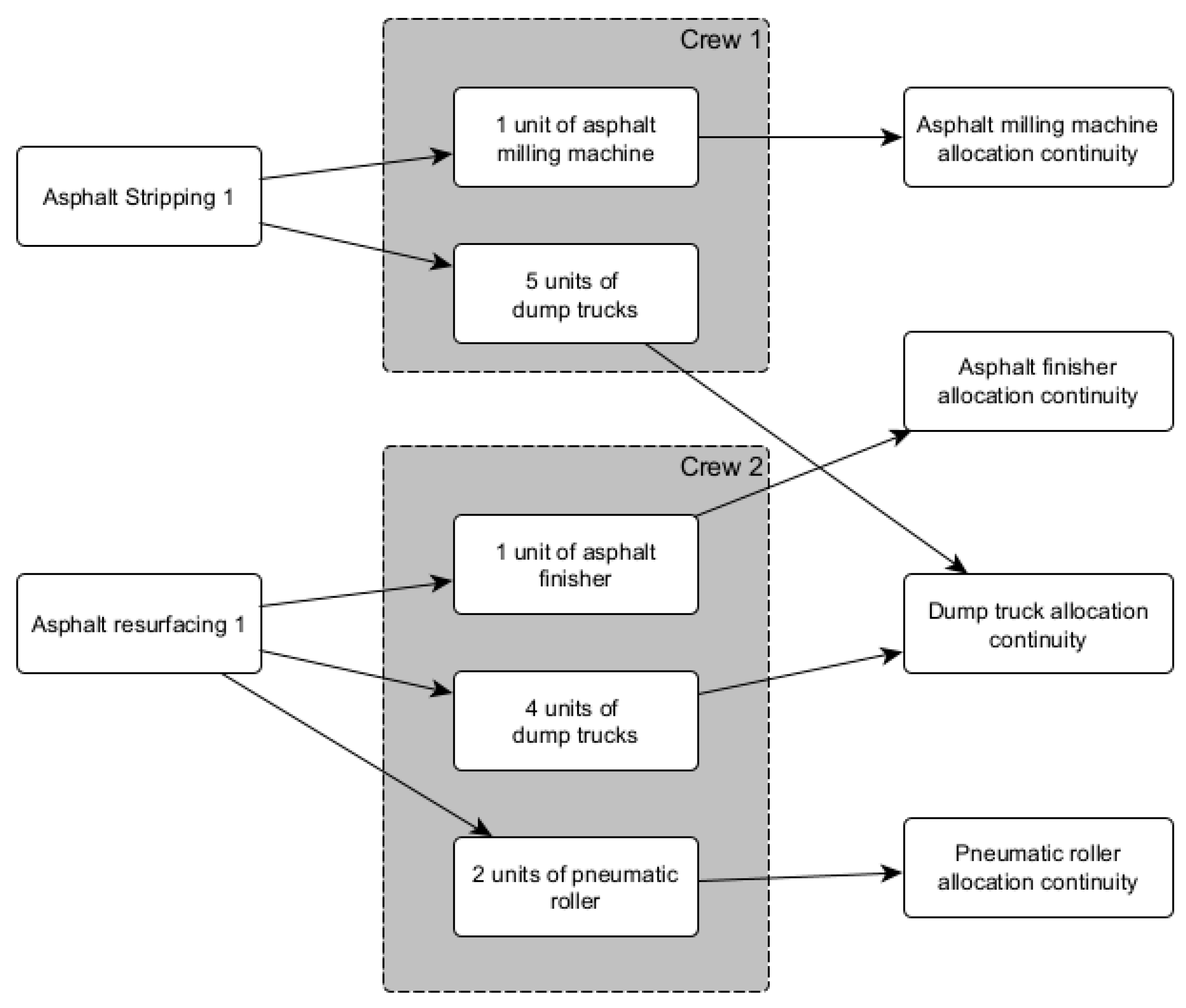
| Activity Name | Crew | Main Equipment | Supporting Equipment |
|---|---|---|---|
| Asphalt stripping | 1 | Asphalt milling machine (AM) | 5 Dump trucks (DT) |
| Asphalt resurfacing | 2 | Asphalt finisher machine (AF) | 4 Dump trucks (DT), 2 pneumatic rollers (PR) |
| Road marking | 3 | Road marking machine (ME) | - |
| Index | Description | Range |
|---|---|---|
| i, m | Index of equipment type | 1 ... number of equipment types |
| j | Index of a road segment | 1 ... number of road segments |
| k | Index of time (day) | 1 ... contract period |
| Variable | Description |
|---|---|
| u | Number of equipment types |
| r | Number of road segments |
| d | Contract period |
| Precedence relationship between main items of equipment. This variable holds the precedence relationship data between predecessor m and successor i in road segment j. It contains values of zero and one. For example, means on the road segment 3, main equipment 1 is the predecessor of main equipment 2. | |
| The number of main items of equipment required to finish an activity. This variable holds the number of main items of equipment i required on the road segment j. means 4 unit-day of main equipment type 1 is required to finish the related activity on road segment 2. If one unit of main equipment type 1 is allocated, the activity will be finished in four days, or if two units of main equipment 1 are allocated, the activity is finished in two days, etc. | |
| The ratio between supporting equipment and main equipment. This variable describes the relationship between supporting equipment i and main equipment m on the road segment j. means that, on the road segment 2, equipment 4 is the supporting equipment of equipment 1, with a ratio of 5:1. | |
| The number of available items of equipment. This variable holds the number of available items of equipment i. |
| No. | Aspect | Scenario 1 | Scenario 2 | Scenario 3 |
|---|---|---|---|---|
| 1 | Solving method | Traditional LSM | Proposed model | Proposed model |
| 2 | Execution order | predetermined | Not predetermined | Not predetermined |
| 3 | Execution sequence | Serial | Parallel | Parallel |
| 4 | Resource profile | Rectangular | Rectangular | Trapezoidal |
| 5 | Resource | Crew | Main and supporting equipment | Main and supporting equipment |
| Road No. | Pavement Stripping | Pavement Overlaying | Road Marking | |||
|---|---|---|---|---|---|---|
| AM (Unit-Day) | DT (Unit-Day) | AF (Unit-Day) | DT (Unit-Day) | PR (Unit-Day) | ME (Unit-Day) | |
| 1 | 2 | 10 | 5 | 20 | 10 | 2 |
| 2 | 5 | 25 | 13 | 52 | 26 | 5 |
| 3 | 3 | 15 | 7 | 28 | 14 | 3 |
| 4 | 2 | 10 | 6 | 24 | 12 | 2 |
| 5 | 3 | 15 | 7 | 28 | 14 | 3 |
| No. | Equipment Type | Amount | |
|---|---|---|---|
| 1 | Asphalt stripping equipment (AM) | 3 | unit |
| 2 | Asphalt finishing equipment (AF) | 3 | unit |
| 3 | Marking equipment (ME) | 1 | unit |
| 4 | Dump truck (DT) | 14 | unit |
| 5 | Pneumatic roller (PR) | 6 | unit |
| No. | Aspect | Scenario 1 | Scenario 2 | Scenario 3 |
|---|---|---|---|---|
| 1 | Idle equipment | 87 unit-day | 9 unit-day | 9 unit-day |
| 2 | Duration | 28 days | 29 days | 25 days |
| 3 | Execution order | predetermined | Not predetermined | Not predetermined |
| 4 | Execution sequence | Serial | Parallel | Parallel |
| 5 | Resource profile | Rectangle | Rectangle | Trapezoid |
| 6 | AM utilization | 2 | 2 | 2 |
| 7 | AF utilization | 2 | 3 | 3 |
| 8 | ME utilization | 2 | 1 | 2 |
| 9 | DT utilization | 14 | 14 | 24 |
| 10 | PR utilization | 4 | 6 | 6 |
Publisher’s Note: MDPI stays neutral with regard to jurisdictional claims in published maps and institutional affiliations. |
© 2021 by the authors. Licensee MDPI, Basel, Switzerland. This article is an open access article distributed under the terms and conditions of the Creative Commons Attribution (CC BY) license (https://creativecommons.org/licenses/by/4.0/).
Share and Cite
Liu, S.-S.; Budiwirawan, A.; Arifin, M.F.A. Non-Sequential Linear Construction Project Scheduling Model for Minimizing Idle Equipment Using Constraint Programming (CP). Mathematics 2021, 9, 2492. https://0-doi-org.brum.beds.ac.uk/10.3390/math9192492
Liu S-S, Budiwirawan A, Arifin MFA. Non-Sequential Linear Construction Project Scheduling Model for Minimizing Idle Equipment Using Constraint Programming (CP). Mathematics. 2021; 9(19):2492. https://0-doi-org.brum.beds.ac.uk/10.3390/math9192492
Chicago/Turabian StyleLiu, Shu-Shun, Agung Budiwirawan, and Muhammad Faizal Ardhiansyah Arifin. 2021. "Non-Sequential Linear Construction Project Scheduling Model for Minimizing Idle Equipment Using Constraint Programming (CP)" Mathematics 9, no. 19: 2492. https://0-doi-org.brum.beds.ac.uk/10.3390/math9192492