An Imitation and Heuristic Method for Scheduling with Subcontracted Resources

Abstract

A scheduling problem with subcontracted resources is widely spread and is associated with the distribution of limited renewable and non-renewable resources, both own and subcontracted ones based on the work’s due dates and the earliest start time. Scheduling’s goal is to reduce the cost of the subcontracted resources. In the paper, application of a few scheduling methods based on scheduling theory and the optimization algorithm is considered; limitations of these methods’ application are highlighted. It is shown that the use of simulation modeling with heuristic rules for allocation of the renewable resources makes it possible to overcome the identified limitations. A new imitation and heuristic method for solving the assigned scheduling problem is proposed. The comparison of the new method with existing ones in terms of the quality of the found solution and performance of the methods is carried out. A case study is presented that allowed a four-fold reduction of the overall subcontracted resources cost in a real project portfolio.

1. Introduction

The problem of business processes and project works scheduling is one of the key problems of organizational system control. Organizational systems are widely spread: examples are enterprises of various industries, multiservice communication networks, and project organizations.

To date, some methods to solve the scheduling problem with resource constraints have been developed depending on the problem statement, restrictions, and objective function. These are scheduling theory and network methods [1,2,3,4,5], simulation and multi-agent modelling methods [6,7], heuristic methods [8,9], and methods based on the application of commercially available solvers [10,11,12,13,14].

According to the machine environment, scheduling problems can be divided into the main following types with the type notation in brackets [15]: identical parallel machines ($Pm$) where work can be performed at any of the machines [1,2,3,4,5,8,9,12,14]; Job shop ($Jm$) where each work has to be processed on each of the machines and all works have different routes [6,7,11,13]; Open shop ($Om$) where each work has to be processed on each of the machines and some of this processing time may be zero [10].

According to the processing restrictions, there are several main constraints specified: release dates ($r_j$), where work $j$ cannot start its processing before its release date [3,4,5]; precedence constraints ($prec$), where one or more works have to be completed before execution of a certain consequent work is allowed [1,2,3,4,5,6,7,8,9,12,13,14]; batch processing ($batch\left(b\right)$), where a machine may be able to process a number of $b$ works simultaneously [11,12]; and breakdowns ($brkdwn$), where a machine may not be permanently available [3,5].

The main objective functions of the scheduling problem are: Makespan minimization ($C_{max}$) is a minimization of the last work’s completion time to leave the system [1,2,3,4,6,7,8,9]; and the weighted number of tardy jobs minimization ($\sum {\omega }_j{U}_j$) [5,11,12,13,14], throughput maximization [10].

In general, the scheduling problem is a problem of work’s sequence definition satisfying the given restrictions and minimizing makespan. A schedule, or calendar plan, is a set of work start dates. Commonly, researchers have investigated the renewable restricted resources that are occupied while a work is being performed and released when the work is over, as in [1,2,4,5,6,8,9,10,11,12,14]. Examples of the renewable resources are personnel, aggregates, vehicles, and other. At the same time, there is an urgent problem to consider non-renewable resources’ distribution, as in [3,7,13]. The non-renewable resources are consumed at the work input and produced at the work output. Examples are raw materials, fuel, finance, and goods.

We consider the scheduling problem on parallel machines in the presence of the orders’ earliest start times and due dates. We have extended the problem by using subcontracted resources’ cost optimization and accounting for restricted non-renewable resources. The optimization of subcontracted resources is relevant either for enterprises with a relatively small set of their own resources, or for enterprises with resources of constrained competence. These enterprises flexibly respond to demand fluctuations in products manufactured or services provided and attract subcontracted resources when it is necessary. Examples are construction companies and project organizations. They need to reduce the engaged subcontractors’ cost while keeping with existing time restrictions to reduce the company’s waste.

The rest of the paper is organized as follows. In Section 2, a literature overview is presented. Notations used are presented in Section 3. In Section 4, a scheduling problem is formulated considering own and subcontracted renewable and non-renewable resources. Application of the scheduling methods to the trial problem and their shortcomings are given in Section 5. In Section 6, we propose an imitation and heuristic method for the problem considered. In Section 7 and Section 8, a case study is presented providing a comparison of the application results of the methods considered. We conclude this research and propose directions for the further work in Section 9.

2. Literature Overview

Network methods for the scheduling problem are introduced in [1,2]. They are intended to determine a critical path and backup time for a work. A PERT method [1] is used when works have a probabilistic duration with due dates. A GERT method [2] extends the PERT method by considering the probabilities of individual works’ implementation. The methods are very useful in the case of precedence relation occurrence. Network methods do not support non-renewable resources’ implementation and restrictions on the works’ earliest start time.

An approximate algorithm proposed in [3] is intended to solve the scheduling problem with restricted renewable and non-renewable resources in the presence of a deadline and restrictions on the earliest start time for a work. The algorithm has two stages. At the first stage, a feasible schedule is calculated based on an assumption that all resources are non-renewable. At the second stage, the renewable resources’ constraints are added to the schedule found and then works are packed to satisfy all resource constraints and minimize the execution time. A disadvantage of the algorithm is that the arrangement solution is excluded from consideration if contradictions arise between the resource constraints and work deadlines. For example, excess availability of the own renewable resources for works on the critical path can exist. In this case, companies can use subcontracted renewable resources, the cost of which needs to be optimized.

For a scheduling optimization problem in a parallel system with identical non-renewable resources and orders’ earliest start dates, two algorithms of the scheduling theory are presented in [4,5]. The algorithms are discussed in detail in Section 5.

A decentralized scheduling approach applied to a job-shop scheduling problem via agent-based simulation is presented in [6,7]. Multi-agent simulation is a popular technique intended to represent decision makers as a community of interacting agents [16]. In this case, each renewable resource and each single work is represented by an agent. The agents interact with each other and allocate the resources to the works by mean of negotiations. In [6], a new control algorithm based on dispatching rules is described. This algorithm is used to assign a score to each agent-resource proposal to agent-work, then the agent-work chooses the highest scored one. The resource score depends on the work’s minimum processing time provided by the current resource compared to all the available alternatives, and the average cycle time of the system. An advantage of the algorithm is simultaneous multi-objective optimization of the system’s throughput and cycle time, with weighted linear convolution of the two into a single objective function. In [7], the schedule is built via self-organization of software agents forming two networks of demands and resources, competing and cooperating on a virtual market. Agents of the basic types are the agents of orders (works), tasks (operations), resources (renewable resources), products (non-renewable resources), as well as the scene agent. Each agent has its own objective function named the satisfaction function, which is a weighted sum of components that meet various criteria. The value of the system’s objective function is refined through the normalized sum of the agents’ objective functions. The scheduling algorithm given in [7] includes a negotiation stage used by agents to build a set of conflicting orders for the resources and a conflict resolution stage, which recursively search for placement options taking into account existing limitations. The main advantages of the agent-based scheduling approach proposed in [7] are the agent’s knowledge base of preferences when assigning resources to operations and the ability to reschedule in real time if the list of available resources or works has changed.

Heuristic scheduling algorithms based on a genetic algorithm are presented in [8,9]. The genetic algorithm (GA) is a popular optimization technique applicable to various application fields proposed by Goldberg [17]. In [8,9], a sequence of works is encoded into a chromosome, a population of the chromosomes is formed to represent a project, and then the population is transformed via genetic operators. Each of the investigations proposes a fitness function of the total project duration that is to be minimized. In [8], the authors introduce a dense gene concept, which is a fixed chromosome section that encodes a sequence of works that uses the available renewable resources in the most optimal way, providing the smallest remainder of free resources. The scarcity of the renewable resource is determined by solving the simplified scheduling problem with assumption that all the resources are non-renewable and calculating the remaining free resources. In [9], a scheduling problem of prefabricated buildings is considered. The authors consider both renewable resources and prefabricated blocks, or non-renewable resources, and their supplies. The GA consists of two stages: first, a schedule is formed with the assumption that the non-renewable resources are in shortage; second, the non-renewable resource supply’s time constraints are added to the schedule and a new search is performed. The advantage of the algorithm presented in [9] is the use of heuristics to generate an initial population that allows a reduction in the number of unfeasible solutions produced by GA.

Commercial solvers were applied to the scheduling problem in [10,11,12,13,14].

OptQuest optimizer is a software that incorporates a combination of metaheuristics, such as scatter search, tabu search, and neural networks [18]. As a part of the AnyLogic modeling system [19], OptQuest is used to solve the multi-objective scheduling problem in [10,11]. A simulation model is used as an objective function for the optimization, which in return determines an optimal configuration of input parameters for the simulation model. Two algorithms of the renewable resources’ allocation based on dispatching rules or on agent negotiation are compared using the OptQuest optimizer in [10]. Controlled variables are the assignment of resources to works, and the objective function is a multi-object function that estimates the total delay of the works and the total consumption of the renewable resources. The authors concluded that the use of the multi-agent approach decreases the resource waiting time for works but does not increase the throughput. The advantage of the study [11] is that energy consumption is considered as a part of the objective function. The author searches for an effective batch size using OptQuest optimizer and then improves the resources’ utilization within the obtained schedule. It is concluded that batch size has a greater impact on the total delay rather than on the energy consumption.

A GA-based solver is embedded into the Tecnomatix Plant Simulation software package [20]. An application of this solver to the scheduling problem is presented in [12,13]. In [12], a flow shop problem is considered with a multi-objective function minimizing the mean flow time and total setup time. The solver optimizes the batch size and sequence of the product batches entering the system. In [13], a real-time job shop scheduling problem is considered with restricted renewable and non-renewable resources and works’ due dates. A simulation model is used to assess the idling of processing equipment and the efficiency of the workshop in terms of throughput. The GA solver is used to allocate the renewable and non-renewable resources to the works. Advantages of the study are consideration of both types of resources and the integration of the scheduling phase into a cloud manufacturing system.

Subcontracted renewable resources are considered in [14]. The authors optimize the schedule cost by allocation of own and subcontracted resources taking into account a time-cost contradiction. The method is discussed in detail in Section 5.

We consider the scheduling problem optimizing not only own renewable resources but also subcontracted ones. The problem’s objective function is cost minimization of the engaged subcontracted resources. The problem restrictions include the time frame of the earliest and latest work start date and a limited amount of the non-renewable resources available.

The goal of the present paper is to develop and assess an imitation and heuristic (IH) method for the scheduling problem with subcontracted resources. We considered two scheduling theory methods of scheduling on parallel machines by V. S. Tanaev and Y. A. Mezentsev to be most suitable for solving the given problem. We also considered application of a commercial solver to the given problem. Use of simulation and heuristics together allows us to overcome the revealed disadvantages of the considered methods. The developed IH method was applied for schedule search in a project company.

3. Notations

3.1. Indices

We consider the following indices:

• $g$ is an index of the renewable resource of the allocated competence, $g=\overline{1,Q_r}$;
• $i$ is an index of the operation or order contained in the project $p$, $i=\overline{1,N_p}$;
• $j$ is an index of the operation or order that cannot be executed at the same time with the order $i$ because they are to be processed by a single machine $g$, $j=\overline{1,N_p}$;
• $k$ is an index of the time interval specified by the time constraints in the V.C. Tanaev method, $k=\overline{1,\beta }$, $\beta \le 2N_p-1$;
• $L$ is an index of the order that can be processed during $E_k$ time interval in the V.C. Tanaev method, $L=\overline{1,n\left(k\right)}$;
• $p$ is an index of the project contained in the portfolio, $p=\overline{1,P}$;
• $r$ is an index of the renewable resource’s competence, $r=\overline{1,R}$;
• $st$ is an index of the dynamic programming stage of the Y.A. Mezentsev algorithm, $st=\overline{1,N_p}$;
• $t$ is an index of the day, $t=\overline{\mathsf{\tau },T}$;
• $v$ is an index of the non-renewable resource, $v=\overline{1,V}$;
• $\eta$ is an index of the iteration stage of the IH algorithm, $\eta =\overline{1,\mathsf{\Psi }}$.

3.2. Sets

We consider the following sets:

• $e_1<e_2<\dots <e_{k+1}$ is a set of the variables ${\mathsf{\tau }}_i^0$ and $d{l}_i$ values in the V.C. Tanaev method;
• $N_k=\left\{i_{k,1}, i_{k,2},\dots , i_{k,n\left(k\right)}\right\}$ is a set of orders that can be processed during $E_k$ interval with index $L$ in the V.C. Tanaev method;
• $P{r}_p$ is a set of operations in the project $p$;
• $Rown$ is a set of own renewable resources;
• $Rsc$ is a set of subcontracted renewable resources;
• $\mathsf{{\rm Z}}\left(t,r\right)$ is a set of indices for operations performed at time $t\ge \tau$ using own or subcontracted renewable resource $r$;
• $\mathsf{{\rm Z}}\left(t,v\right)$ is a set of indices for operations performed at time $t\ge \tau$ using non-renewable resource $v$;
• $\mathsf{\Theta }\left(t,r\right)$ is a set of indices for operations performed at time $t\ge \tau$ using own resource $r$;
• $\mathsf{{\rm Y}}\left(t,r\right)$ is a set of indices for operations performed at time $t\ge \tau$ using subcontracted renewable resource $r$.

3.3. Parameters

We identified the following parameters:

• $c_{p,i,r}$ is a duration of the time interval $M_{p,i,r}\left(\eta \right)$ in the IH algorithm;
• $d_i>0$ is an operation duration in case of one project in the portfolio, i.e., $P=1$;
• $d{l}_i>0$ is a deadline for processing the order $i$; it can be calculated as: $d{l}_i={\tau }_i^1+d_i$;
• $d_{p,i}>0$ is a duration of the operation $i$ of the project $p$;
• $E_k=\left(e_k;e_{k+1}\right]$ is a time interval specified by time constraints in the V.C. Tanaev method, $E_k\subseteq \left({\mathsf{\tau }}_i^0,d{l}_i\right]$;
• $f_{g,st}\left({\tau }_{st}^0,d_{st},y_{g,st}\right)$ is a completion time of the order $i$ processed via the machine or renewable resource $g$ at the stage $st$ in the Y.A. Mezentsev algorithm;
• $Ft$ is a total cost of the subcontracted renewable resources;
• $H \mathrm{and} K^{\prime }$ are parameters of the Y.A. Mezentsev algorithm, they are intended to drop out some feasible solutions at each search stage to decrease the searching time;
• $Kres$ is a total cost of the used resources, own and subcontracted ones;
• $Ksc$ is a predefined limit of the cost of subcontracted renewable resources;
• $M=\underset{k}{\max }n\left(k\right)$ is a quantity of machines or renewable resources, both own and subcontracted, required to process orders in the V.C. Tanaev method, $n\left(k\right)\le M$;
• $M^{\prime }$ is the quantity of the needed subcontracted resources in the V.C. Tanaev method, $M^{\prime }\le \left(M-Q_r\right)$;
• $ML$ is an arbitrarily assumed, sufficiently large constant in the Lingo method;
• $N$ is the number of operations of the project portfolio;
• $N_{st}$ is the current amount of the developed schedules at the stage $st$ in the Y.A. Mezentsev algorithm;
• $n\left(k\right)$ is the quantity of all the orders constituting the $N_k$ set in the V.C. Tanaev method;
• $Q_r$ is the available quantity of the own renewable resource with competence $r$;
• $Q_{t,v}$ is the current quantity of each non-renewable resource $v$ at time $t$;
• $q_{p,i,r}\ge 0$ is the required amount of renewable resources of allocated competence $r$ to perform the operation $i$ of the project $p$; $q_{p,i,r}=0$ when the renewable resource $r$ is not required to process the operation $i$ of the project $p$;
• $q_{p,i,v}^{-}\le 0$ and $q_{p,i,v}^{+}\ge 0$ are the amounts of non-renewable resource $v$ consumed when the operation $i$ of the project $p$ starts and produced when the operation $i$ ends, respectively; $q_{p,i,v}^{-}=0$ when the non-renewable resource $v$ is not required to start the operation $i$ of the project $p$; the variable $q_{p,i,v}^{+}=0$ when the non-renewable resource $v$ is not produced as an outcome of the operation $i$ of the project $p$;
• $S{C}_{p,t,r}$ is a cost of the subcontracted resource of allocated competence $r$ engaged in the project $p$ at the time $t$;
• $s{r}_{i,r}$ is the daily cost of performing the operation $i$ using a unit quantity of the renewable resource $r$ in case of one project in the portfolio, i.e., $P=1$;
• $s{r}_{p,i,r}\ge 0$ is the daily cost of performing the operation $i$ of the project $p$ using a unit quantity of the renewable resource of allocated competence $r$;
• $s{r^{\prime }}_{p,i,r}\ge 0$ is the total cost of performing the operation $i$ of the project $p$ using a subcontracted renewable resource $r$;
• $Tdl$ is the global project’s deadline that must not be exceeded, $Tdl=\underset{i}{\max }d{l}_i$;
• $U_{p,t,r}$ is the percentage utilization of the renewable resource $r$ engaged in the project $p$ at the time $t$.
• $U_{p,i,r}^0\left(\eta \right)$ is the average utilization of the renewable resource $r$ for the operation $i$ of the project $p$ during the time interval ${\delta }_{p,i,r}\left(\eta \right)$ in the IH algorithm;
• $U_{p,i,r}^{-}\left(\eta \right)$ is the average utilization of the renewable resource $r$ for the operation $i$ of the project $p$ during the time interval ${\delta }_{p,i,r}^{-}\left(\eta \right)$ in the IH algorithm;
• $U_{p,i,r}^{+}\left(\eta \right)$ is the average utilization of the renewable resource $r$ for the operation $i$ of the project $p$ during the time interval ${\delta }_{p,i,r}^{+}\left(\eta \right)$ in the IH algorithm;
• ${\Delta }_k=e_{k+1}-$ $e_k$ is the duration of the time interval $E_k$ in the V.C. Tanaev method;
• ${\delta }_{p,i,r}\left(\eta \right)$ is the time interval where the utilization percentage of the renewable resource $r$ for the operation $i$ of the project $p$ is equal to 100%, $U_{p,i,r}^0\left(\eta \right)=100\%$, in the IH algorithm;
• ${\delta }_{p,i,r}^{-}\left(\eta \right)$ is the time interval ${\delta }_{p,i,r}\left(\eta \right)$ shifted to the left on the time axis in the IH algorithm;
• ${\delta }_{p,i,r}^{+}\left(\eta \right)$ is the time interval ${\delta }_{p,i,r}\left(\eta \right)$ shifted to the right on the time axis in the IH algorithm;
• ${\lambda }_{g,i}$ is the cost of processing the order $i$ by the resource $g$;
• ${\mu }_g\left(t\right)$ is a function that shows the presence of subcontracted resources $g$ at the time $t$, $g=\overline{Q_r,M}$;
• ${\xi }_{p,i,r}$ is a threshold of the $s{r^{\prime }}_{p,i,r}$ total cost of performing the operation $i$ of the project $p$ using a subcontracted renewable resource $r$.
• $\sigma \left(t\right)$ is a function of orders allocated to machines or renewable resources in the V.C. Tanaev method;
• ${\tau }_{p,i}^0\ge \tau$ and ${\tau }_{p,i}^1\ge \tau$ are the earliest and latest possible start times given for the operation $i$ of the project $p$; ${\tau }_{p,i}^0={\tau }_{p,i}^1=\tau$ if the operation $i$ is only allowed to start at the time $\tau$;
• ${\tau }_i^0$ and ${\tau }_i^1$ are orders’ earliest and latest possible start times in case of one project in the portfolio, $P=1$;
• ${\widehat{\tau }}_{g,i}$ is the actual delay between start of the $i$-th order on the $g$-th machine upon the previous order completion in the Y.A. Mezentsev algorithm;
• ${\phi }_{g,st}\left({\tau }_i^0,d_i,y_{g,i}\right), i=\overline{1,st}$ is the completion time by the resource $g$ for all the orders that exist at the stages from the first to the $st$-th in the Y.A. Mezentsev algorithm;
• ${\phi }_{st}\left({\tau }_i^0,d_i,y_{g,i}\right), i=\overline{1,st}$ is the minimal completion time for all the orders existing at the stages from the first to the $st$-th in the Y.A. Mezentsev algorithm;
• $\omega$ is the cost of processing the order per time unit in conventional units;
• $\mathsf{\Psi }$ is the predefined maximum number of the IH algorithm steps.

3.4. Decision Variables

The decision variables may vary regarding the different scheduling problem statements. We identify the following decision variables connected with the problem:

• $S_{k,g}\left(t\right)$ are integer variables of a sequence of orders to perform by each renewable resource $g$ at each time interval $E_k$ for the scheduling problem given in Section 5.2;
• $x_{p,i}\in \left\{\tau ,\dots ,T\right\}$ are integer variables of the operation start times for the scheduling problem given in Section 4;
• $x_i\in \left\{\tau ,\dots ,T\right\}$ are integer variables of the operation start times given in Section 5.3 in case of one project in the portfolio, i.e., $P=1$;
• $y_{g,i}$ are Boolean variables for allocating the order $i$ to the machine $g$ for the problems given in Section 5.1, Section 5.2 and Section 5.3. The variable assumes a value of 1 if the order $i$ is to be executed by the machine $g$; otherwise, it equals 0. In Section 5.3, we assume that the machine $g$ can be an own or subcontracted one;
• ${\epsilon }_{i,j}$ are binary variables for the scheduling problem given in Section 5.3. The variable indicates orders that cannot be executed at the same time because they are to be processed by a single machine $g$. The variable ${\epsilon }_{i,j}$ equals 1 if the order $i$ is to be completed before the order $j$; otherwise, it equals 0; $\left(i,j\right)\in P{r}_p$.

4. Scheduling Problem Statement

The scheduling problem statement is given by the authors in [21]. Below are the key points. The notations are presented in Section 3.

We assume that a set of operations in each project $p$ appears in order of increasing of the operation’s cost $s{r}_{p,i,r};$ $s{r}_{p,i,r}=0$ if the subcontracted resource $r$ is not required by the operation $i$ of the project $p$.

We denote the set of indices for the operations performed at the time $t\ge \tau$ utilizing the renewable resource $r$ as follows:

$$\mathsf{{\rm Z}}\left(t,r\right)=\left\{i\in \left[1,N_p\right]│ x_{p,i}\le t<x_{p,i}+d_{p,i} \& q_{p,i,r}\ne 0 \& p\in \left[1,P\right]\right\}$$

(1)

We denote the set of indices for the operations performed at the time $t\ge \tau$ utilizing the non-renewable resource $v$ as follows:

$$\mathsf{{\rm Z}}\left(t,v\right)=\left\{i\in \left[1,N_p\right]│ x_{p,i}\le t<x_{p,i}+d_{p,i} \& q_{p,i,v}^{-}\ne 0 \& p\in \left[1,P\right]\right\}.$$

(2)

We denote the set of indices for the operations performed at the time $t\ge \tau$ utilizing the own renewable resource $r$ within the available amount $Q_r$:

$$\mathsf{\Theta }\left(t,r\right)=\{i\in {\rm Z}\left(t,r\right)│ {\sum }_{p\in \left[1,P\right]}{\sum }_i{q}_{p,i,r}\le Q_r\}.$$

(3)

The set of indices for the operations performed at the time $t\ge \tau$ utilizing the subcontract resource $r$ is defined as follows:

$$\mathsf{{\rm Y}}\left(t,r\right)=\mathsf{{\rm Z}}\left(t,r\right)\backslash \mathsf{\Theta }\left(t,r\right)=\left\{i\in \left[1,N_p\right]│i\in \mathsf{{\rm Z}}\left(t,r\right) \& i\notin \mathsf{\Theta }\left(t,r\right)\right\}.$$

(4)

The percentage utilization of the resource $r$ engaged in the project $p$ at the time $t$ is defined as follows:

$$U_{p,t,r}=\{\begin{array}{c}\left(\sum _{i\in \mathsf{\Theta }\left(t,r\right)}{q}_{p,i,r}/Q_r\right)·100\%, i\in \mathsf{\Theta }\left(t,r\right),\\ 100\%, i\in \mathsf{{\rm Y}}\left(t,r\right).\end{array}$$

(5)

The cost of the subcontract resource of an allocated competence $r$ involved in the project $p$ at the time $t$ is defined by the formula:

$$S{C}_{p,t,r}={\sum }_{i\in \mathsf{{\rm Y}}\left(t,r\right)}s{r}_{p,i,r}\cdot q_{p,i,r}.$$

(6)

The current volume of the non-renewable resource $v$ at the time $t$ is defined as:

$$Q_{t,v}=Q_{\tau ,v}+{\sum }_{\alpha =\tau }^t{\sum }_{p=1}^P{\sum }_{\begin{array}{c}i\in P{r}_p\\ \wedge \alpha =x_{p,i}\end{array}}{q}_{p,i,v}^{-}+{\sum }_{\alpha =\tau }^t{\sum }_{p=1}^P{\sum }_{\begin{array}{c}i\in P{r}_p\\ \wedge \alpha =x_{p,i}+d_{p,i}\end{array}}{q}_{p,i,v}^{+}.$$

(7)

The scheduling problem can be formalized as follows:

$$Ft={\sum }_{p=1}^P{\sum }_{t=\tau }^T{\sum }_{r=1}^{R}S{C}_{p,t,r}\to min,$$

(8)

$${\sum }_{p=1}^P{\sum }_{\begin{array}{c}i\in Z\left(t,v\right)\\ \wedge t=x_{p,i}\end{array}}\left|q_{p,i,v}^{-}\right|\le Q_{t,v}, \forall t=\overline{\mathsf{\tau },T}, \forall v=\overline{1,V},$$

(9)

$${\tau }_{p,i}^0\le x_{p,i}\le {\tau }_{p,i}^1, \forall p=\overline{1,P}, \forall i=\overline{1,N_p}.$$

(10)

The objective function (8) minimizes the total cost of the subcontracted resources in the case of exceeding the availability of the own ones. The constraint (9) ensures availability of the required amount of non-renewable resources at the time of the operation start. The constraint (10) imposes a time frame on the start dates of the operations.

5. Scheduling Methods Application

We consider the schedule optimization problem for the parallel system having identical machines in the presence of delays processing the orders. The problem is one of the closest problems studied by the scheduling theory. According to [15], the problem is formalized as follows: $Pm/r_j/C_{max}$. For the problem, a parametric algorithm of dynamic programming with an alternative dropout option was proposed by Y. A. Mezentsev et al. [4].

Another closest problem studied by the scheduling theory is a parallel system schedule optimization using identical machines in the presence of orders’ due dates. The problem is formalized as follows: $Pm/brkdwn,r_j/\sum {\omega }_j{U}_j$. As a solution to the problem, a schedule construction algorithm using the given due dates is proposed by V. S. Tanaev et al. [5].

We also considered Lingo commercial solver’s application to the scheduling problem according to the scheme given in [14]. Here, the problem is modelled as a mixed binary linear program that minimizes the project cost, including subcontracted and own resources cost.

We applied the considered algorithms to solve a trial small-scale scheduling problem using two own renewable resources $Q_1=2$ of the same competence $R=1$, and one project $P=1$ with the number of the operations $N_1=7$. Seven orders, or operations, are fed at a different time into a parallel system with two identical machines, or renewable resources.

Table 1. Initial information of the trial scheduling problem.

$\mathbf{Order} \mathbf{Number}, \mathit{i}$	$\mathbf{Order} \mathbf{Duration}, {\mathit{d}}_{\mathit{i}}$	$\mathbf{Earliest} \mathbf{Start} \mathbf{Time}, {\mathit{\tau }}^0{}_{\mathit{i}}$	$\mathbf{Deadline}, \mathit{d}{\mathit{l}}_{\mathit{i}}$
1	2	0	3
2	3	0	4
3	2	1	4
4	4	2	7
5	3	3	7
6	2	5	8
7	4	5	10

contains the initial information about the operation’s duration and time frame between order processing’s earliest possible start and latest finish. We assume the operations are ordered by the earliest start time.

The progress of solving the problem is given below.

5.1. Method Developed by Y. A. Mezentsev

We applied a parametric dynamic programming algorithm with the optional exclusion of the found alternatives to the considered scheduling problem. The notations are given in Section 3. The decision variables are Boolean variables $y_{g,i}$ allocating the order $i$ to the machine $g$.

The dynamic algorithm variables can be calculated as given in the study [4]:

$$f_{g,st}\left({\tau }_{st}^0,d_{st},y_{g,st}\right)=\underset{}{\max }\left\{0,\left[{\tau }_{st}^0{y}_{g,st}-{\phi }_{g,st-1}\left({\tau }_{st-1}^0,d_i,y_{g,i}\right)\right]\right\}+d_{st}{y}_{g,st},$$

(11)

$${\phi }_{g,st}\left({\tau }_i^0,d_i,y_{g,i}\right)=\left\{f_{g,st}\left({\tau }_{st}^0,d_{st},y_{g,st}\right)+{\phi }_{g,st-1}\left({\tau }_i^0,d_i,y_{g,i}\right)\right\}, i=\overline{1,st-1},$$

(12)

$${\phi }_{st}\left({\tau }_i^0,d_i,y_{g,i}\right)=\underset{g}{\max }\left\{{\phi }_{g,st}\left({\tau }_{st}^0,d_i,y_{g,i}\right)\right\},i=\overline{1,st}.$$

(13)

The parametric algorithm includes the following stages:

• Input of the initial data $\left({\tau }_i^0,d_i, d{l}_i\right)$, $i=\overline{1,N_p}$ and $H, K^{\prime }, Q_r$, and $N_p$ parameters. Set ${\phi }_{g,0}\left({\tau }_0^0,d_i,y_{g,i}\right)=0$, $st=0$;
• $st=st+1$;
• If $st>N_p$ then go to Point 7;
• Generate all the feasible schedules and calculate $f_{g,st}\left({\tau }_{st}^0,d_{st},y_{g,st}\right)$ and the schedule length ${\phi }_{g,st}\left({\tau }_i^0,d_i,y_{g,i}\right)$;
• Check the number of the generated schedules $N_{st}$. If $N_{st}\le K^{\prime }$ then go to Point 2; otherwise, go to Point 6;
• Discard $Q_r{}^{H-1}$ out of the schedules generated at Point 4 with the maximum schedule length ${\phi }_{g,st}\left({\tau }_i^0,d_i,y_{g,i}\right)$. Go to Point 2;
• Choose the schedules with the minimum makespan. Determine the calendar plan by reverse dynamic programming.

We consider application of the parametric algorithm to the trial scheduling problem given in Table 1. Examples of the calculated algorithm characteristics are given in

Table 2. Results of the first algorithm stage completion.

Stage 1	${\mathit{x}}_{1,1}$	${\mathit{x}}_{2,1}$	${\mathit{f}}_{\mathit{g},1}$	${\mathit{\phi }}_{\mathit{g},1}={\mathit{f}}_{\mathit{g},1}, {\mathit{\phi }}_1=\underset{\mathit{g}}{\mathbf{max}}\left\{{\mathit{\phi }}_{\mathit{g},1}\right\}$
Order 1	1	0	(max{0,0-0} + 2,0) = (2,0)	${\phi }_1=$ max{2,0} = 2
	0	1	(0,max{0,0-0} + 2) = (0,2)	${\phi }_1=$ max{0,2} = 2

and

Table 3. Results of the last algorithm stage completion.

Stage 7	${\mathit{x}}_{1,1}$	${\mathit{x}}_{2,1}$	${\mathit{x}}_{1,2}$	${\mathit{x}}_{2,2}$	${\mathit{x}}_{1,3}$	${\mathit{x}}_{2,3}$	${\mathit{x}}_{1,4}$	${\mathit{x}}_{2,4}$	${\mathit{x}}_{1,5}$	${\mathit{x}}_{2,5}$	${\mathit{x}}_{1,6}$	${\mathit{x}}_{2,6}$	${\mathit{x}}_{1,7}$	${\mathit{x}}_{2,7}$	${\mathit{f}}_{\mathit{g},7}$	${\mathit{\phi }}_{\mathit{g},7}=\left\{{\mathit{f}}_{\mathit{g},7}+{\mathit{\phi }}_{\mathit{g},6}\right\},$ ${\mathit{\phi }}_7=\underset{\mathit{g}}{\mathbf{max}}\left\{{\mathit{\phi }}_{\mathit{g},7}\right\}$
Order 1+ Order 2+ Order 3+ Order 4+ Order 5+ Order 6+ Order 7	1	0	0	1	1	0	0	1	1	0	0	1	1	0	(max{0,5-8} + 4,0) = (4,0)	max{2 + 3 + 0 + 0 + 3 + 0 + 4, 0 + 0 + 3 + 4 + 0 + 2 + 0} = 12
	1	0	0	1	1	0	0	1	1	0	0	1	0	1	(0,max{0,5-9} + 4) = (0,4)	max{2 + 3 + 0 + 0 + 3 + 0 + 0, 0 + 0 + 3 + 4 + 0 + 2 + 4} = 13
	1	0	0	1	1	0	0	1	1	0	1	0	1	0	(max{0,5-9} + 4,0) = (4,0)	max{2 + 0 + 2 + 0 + 3 + 2 + 4, 0 + 3 + 0 + 4 + 0 + 0 + 0} = 13
	1	0	0	1	1	0	0	1	1	0	1	0	0	1	(0,max{0,5-7} + 4) = (0,4)	max{2 + 0 + 2 + 0 + 3 + 2 + 0, 0 + 3 + 0 + 4 + 0 + 0 + 4} = 11
	1	0	0	1	1	1	0	0	1	0	0	1	1	0	(max{0,5-7} + 4,0) = (4,0)	max{2 + 0 + 2 + 0 + 3 + 0 + 4, 0 + 3 + 0 + 4 + 0 + 2 + 0} = 11
	0	1	1	0	0	1	1	0	1	0	0	1	0	1	(0,max{0,5-9} + 4) = (0,4)	max{2 + 0 + 2 + 0 + 3 + 0 + 0, 0 + 3 + 0 + 4 + 0 + 2 + 4} = 13
	0	1	1	0	0	1	1	0	0	1	1	0	1	0	(max{0,5-9} + 4,0) = (4,0)	max{0 + 3 + 0 + 4 + 0 + 2 + 4, 2 + 0 + 2 + 0 + 3 + 0 + 0} = 13
	0	1	1	0	0	1	1	0	0	1	1	0	0	1	(0,max{0,5-7} + 4) = (0,4)	max{0 + 3 + 0 + 4 + 0 + 2 + 0, 2 + 0 + 2 + 0 + 3 + 0 + 4} = 11
	0	1	1	0	0	1	1	0	0	1	0	1	1	0	(max{0,5-7} + 4,0) = (4,0)	max{0 + 3 + 0 + 4 + 0 + 0 + 4, 2 + 0 + 2 + 0 + 3 + 2 + 0} = 11
	0	1	1	0	0	1	1	0	0	1	0	1	0	1	(0,max{0,5-9} + 4) = (0,4)	max{0 + 3 + 0 + 4 + 0 + 0 + 0, 2 + 0 + 2 + 0 + 3 + 2 + 4} = 13
	0	1	1	0	0	1	1	0	0	1	1	0	1	0	(max{0,5-9} + 4,0) = (4,0)	max{0 + 0 + 3 + 4 + 0 + 2 + 4, 2 + 3 + 0 + 0 + 3 + 0 + 0} = 13
	0	1	1	0	0	1	1	0	1	0	0	1	0	1	(0,max{0,5-9} + 4) = (0,4)	max{2 + 3 + 0 + 0 + 3 + 0 + 0, 0 + 0 + 3 + 4 + 0 + 2 + 4} = 13

for the first and last algorithm stages. We set $H=2$, $K^{\prime }=2^2=4$.

Table 3 contains the dark filled cells connected to the schedules providing the minimum local makespan on the given stage.

Table 4. Schedules with minimal makespan.

Schedule	${\mathit{x}}_{1,1}$	${\mathit{x}}_{2,1}$	${\mathit{x}}_{1,2}$	${\mathit{x}}_{2,2}$	${\mathit{x}}_{1,3}$	${\mathit{x}}_{2,3}$	${\mathit{x}}_{1,4}$	${\mathit{x}}_{2,4}$	${\mathit{x}}_{1,5}$	${\mathit{x}}_{2,5}$	${\mathit{x}}_{1,6}$	${\mathit{x}}_{2,6}$	${\mathit{x}}_{1,7}$	${\mathit{x}}_{2,7}$	${\mathit{\phi }}_7$
1	1	0	0	1	1	0	0	1	1	0	1	0	0	1	11
2	1	0	0	1	1	0	0	1	1	0	0	1	1	0	11
3	0	1	1	0	0	1	1	0	0	1	1	0	0	1	11
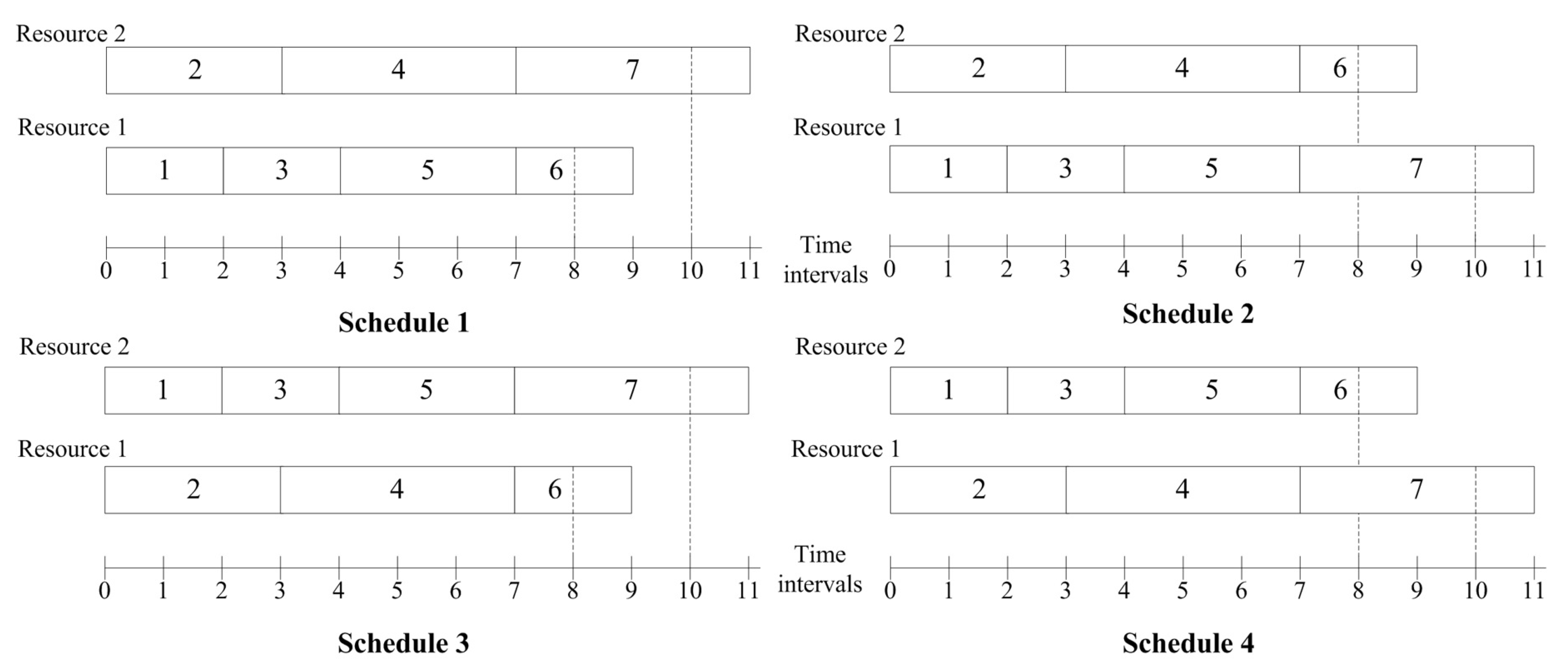
4	0	1	1	0	0	1	1	0	0	1	0	1	1	0	11

contains the four schedules identified as the solutions of the given small-scale scheduling problem.

Since the machines are identical, schedule 1 is equal to schedule 4 and schedule 2 is equal to schedule 3. Schedules 1 and 2 differ by two last orders allocated to the opposite machines. All of the schedules reveal deadline violation on orders 6 and 7.

The obtained schedules are shown in Figure 1 in the form of a Gantt chart.

As we can see, the schedules found by the Y. A. Mezentsev method for a parallel system with identical machines and orders’ earliest start time do not support the orders’ due date. Subcontracted resources are not considered by the method. Thus, $Ft=0$ for the schedule found by Y. A. Mezentsev.

5.2. Method Developed by V. C. Tanaev

We considered an algorithm implemented by V. C. Tanaev. The notations used are given in Section 3.

The decision variables are schedules $S_{k,g}\left(t\right)$ for each resource $g$ at each time interval $E_k$. These are integer type variables.

Two cases can occur: (1) $M\le Q_r$ if the existing machines are enough to process all the orders within time intervals $E_k$; (2) $M>Q_r$ if the existing machines are not enough to process all the orders at the $E_k$ time intervals and it is necessary to attract an amount $M^{\prime }\le \left(M-Q_r\right)$ of subcontracted machines.

An algorithm is given in [5] and contains the following stages. We modified the algorithm by adding the stages 4 to 7 to reduce the number of interruptions:

• $k=0$;
• The next index of the time interval: $k=k+1$. If $k>\beta$ then go to Point 9; otherwise, perform the following actions. Form a set of orders $N_k=\left\{i_{k,1}, i_{k,2},\dots , i_{k,n\left(k\right)}\right\}$, which can be processed at the $E_k$ interval. The orders are sorted by descending the cost of the processing per time unit;
• If $\underset{i\in N_k}{\min }\left\{d_i\right\}<{\Delta }_k$ then go to Point 8; otherwise, go to Point 4;
• Start to browse a set of machines with given competence: $g=0$;
• The next index of the machine: $g=g+1$. If ($g>M$) OR ($N_k=\varnothing$), then go to Point 2; otherwise, start to browse the set of orders from the beginning $N_k$: $L=0;$
• The next index of the order: $L=L+1$. If $L>n\left(k\right)$, then go to Point 5; otherwise, go to Point 7;
• Assign the machine $g$ to the order $i_{k,L}\in N_k$ and form the schedule $S_{k,g}\left(t\right)$ at the $E_k$ time interval:
  • If $\left(k=1\right)$ OR ($k\ne 1$ AND the order $i_{k,L}$ at the previous time interval $E_{k-1}$ has not been assigned to the machine $g^{\prime }\ne g$) OR ($k\ne 1$ AND the order $i_{k,L}$ at the previous time interval $E_{k-1}$ has been assigned to the machine $g^{\prime }\ne g,$ $g^{\prime }>Q_r$ AND $n\left(k\right)\le Q_r$), then assign the machine $g$ to the order $i_{k,L}$:
    • $d_i=d_i-{\Delta }_k$, $S_{k,g}\left(t\right)=i_{k,L}$, where $t=\left(e_k; e_{k+1}\right]$;
    • Eliminate the order $i_{k,L}$ from the set $N_k$. Go to Point 5;
  • If ($k\ne 1$ AND the order $i_{k,L}$ at the previous time interval $E_{k-1}$ has been assigned to the machine $g^{\prime }\ne g,$ $g^{\prime }\le Q_r$) OR ($k\ne 1$ AND the order $i_{k,L}$ at the previous time interval $E_{k-1}$ has been assigned to the machine $g^{\prime }\ne g$ and $g^{\prime }>Q_r$ AND $n\left(k\right)>Q_r$), then go to Point 6;
• Calculate the processing duration of all the orders constituting the $N_k$ set according to the formula: $d_i{}^{\prime }≔\{\begin{array}{c}{d}_i,d_i<{\Delta }_k \\ {\Delta }_k,d_i\ge {\Delta }_k\end{array}, i\in N_k$. Apply a packing algorithm intended to assign the $N_k$ set orders having $d_i{}^{\prime }$ durations to the set $M$ machines for the $E_k$ time interval. At this stage, we consider the following statements are true: $d_i{}^{\prime }\le {\Delta }_k$, $i\in N_k$ and $\sum _{i\in N_k}{d}_i{}^{\prime }\le M{\Delta }_k$:
  • Calculate at the time interval $\left(e_k; e_k+M{\Delta }_k\right]$ a function $\sigma \left(t\right)$, where:
    • $\sigma \left(t\right)=i_{k,1}$ at the time interval $\left(e_k; e_k+d_{i,k,1}\right]$;
    • $\sigma \left(t\right)=i_{k,\alpha }$ at the time interval $(e_k+\sum _{\alpha =1}^{\mathsf{A}-1}{d}_{i,k,\alpha }; e_k+\sum _{\alpha =1}^{\mathsf{A}}{d}_{i,k,\alpha }]$,$\mathsf{A}=\overline{2,n\left(k\right)}$;
    • if $\sum _{i\in N_k}{d}_i<M{\Delta }_k$, then $\sigma \left(t\right)=0$ at the time interval
    • $(e_k+\sum _{i\in N_k}{d}_i; e_k+M{\Delta }_k]$;
  • Form the schedule $S_{k,g}\left(t\right)=\sigma \left(t+\left(g-1\right){\Delta }_k\right)$, $g=\overline{1,M}$;
  • $d_i=d_i-d_i{}^{\prime }$, $i\in N_k$. Go to Point 2;
• The end of the algorithm.

We used the algorithm to solve the scheduling problem given in Table 1. We sorted the set $N_p$ orders according to the information given in Table 1.

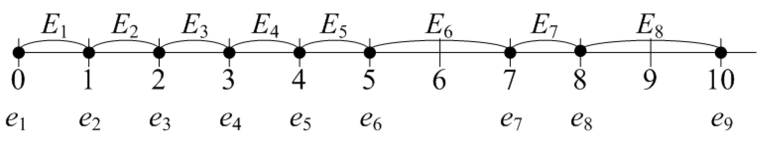
We allocated time marks $\left\{e_{\beta +1}\right\}$, $\beta +1=9$ to form a set of time intervals $\left\{E_k\right\}$, where $k=\overline{1,8}$ (Figure 2).

Results of the method’s execution upon the trial problem are given in

Table 5. Schedule search with orders’ due date by the V. S. Tanaev method.

Interval ${\mathit{E}}_{\mathit{k}}$ and Its Length ${\mathbf{\Delta }}_{\mathit{k}}$	Set ${\mathit{N}}_{\mathit{k}}$	$\mathbf{Schedule} {\mathit{S}}_{\mathit{k},\mathit{g}}, \mathit{g}=\overline{1,\mathit{M}}$	$\mathbf{Duration} {\mathit{d}}_{\mathit{i}},$ $\mathit{i}\in {\mathit{N}}_{\mathit{k}}$	$\mathbf{Function} \mathit{\sigma }\left(\mathit{t}\right)$ $\mathbf{Where} \underset{\mathit{i}\in {\mathit{N}}_{\mathit{k}}}{\mathbf{min}}\left\{{\mathit{d}}_{\mathit{i}}\right\}<{\mathbf{\Delta }}_{\mathit{k}}$
$E_1=$ (0;1] ${\Delta }_1=1$	$N_1=\left\{i_1, i_2\right\}$	$S_{1,1}\left(t\right)=i_1$ $S_{1,2}\left(t\right)=i_2$ $S_{1,3}\left(t\right)=0$	$t_1=$ 2 − 1 = 1 $t_2=$ 3 − 1 = 2
$E_2=$ (1;2] ${\Delta }_2=1$	$N_2=\left\{i_1, i_2,i_3\right\}$	$S_{2,1}\left(t\right)=i_1$ $S_{2,2}\left(t\right)=i_2$ $S_{2,3}\left(t\right)=i_3$	$t_1=$ 1 − 1 = 0 $t_2=$ 2 − 1 = 1 $t_3=$ 2 − 1 = 1
$E_3=$ (4;5] ${\Delta }_3=1$	$N_3=\left\{i_2,i_3,i_4\right\}$	$S_{3,1}\left(t\right)=i_4$ $S_{3,2}\left(t\right)=i_2$ $S_{3,3}\left(t\right)=i_3$	$t_4=$ 4 − 1 = 3 $t_2=$ 1 − 1 = 0 $t_3=$ 1 − 1 = 0
$E_4=$ (3;4] ${\Delta }_{4 }=1$	$N_4=\left\{i_4, i_5\right\}$	$S_{4,1}\left(t\right)=i_4$ $S_{4,2}\left(t\right)=i_5$ $S_{4,3}\left(t\right)=0$	$t_4=$ 3 − 1 = 2 $t_5=$ 3 − 1 = 2
$E_5=$ (4;5] ${\Delta }_5=1$	$N_5=\left\{i_4, i_5\right\}$	$S_{5,1}\left(t\right)=i_4$ $S_{5,2}\left(t\right)=i_5$ $S_{5,3}\left(t\right)=0$	$t_4=$ 2 − 1 = 1 $t_5=$ 2 − 1 = 1
$E_6=$ (5;7] ${\Delta }_{6 }=2$	$N_6=\left\{i_4, i_5,i_6, i_7\right\}$	$S_{6,1}\left(t\right)=\{\begin{array}{c}{i}_4 if t\in \left(5;6\right]\\ i_5 if t\in \left(6;7\right]\end{array}$ $S_{6,2}\left(t\right)=i_6$ $S_{6,3}\left(t\right)=i_7$	$t_4=$ 1 − 1 = 0 $t_5=$ 1 − 1 = 0 $t_6=$ 2 − 2 = 0 $t_7=$ 4 − 2 = 2	$\sigma \left(t\right)=\{\begin{array}{c}\begin{array}{c}{i}_4 if t\in \left(5;6\right]\\ i_5 if t\in \left(6;7\right]\end{array}\\ i_6 if t\in \left(7;9\right]\\ i_7 if t\in \left(9;11\right]\end{array}$
$E_7=$ (7;8] ${\Delta }_7=1$	$N_7=\left\{i_7\right\}$	$S_{7,1}\left(t\right)=i_7$ $S_{7,2}\left(t\right)=0$ $S_{7,3}\left(t\right)=0$	$t_7=$ 2 − 1 = 1
$E_8=$ (8;10] ${\Delta }_8=2$	$N_8=\left\{i_7\right\}$	$S_{8,1}\left(t\right)=\{\begin{array}{c}{i}_7 if t\in \left(8;9\right]\\ 0 if t\in \left(9;10\right]\end{array}$ $S_{8,2}\left(t\right)=0$ $S_{8,3}\left(t\right)=0$	$t_7=$ 1 − 1 = 0	$\sigma \left(t\right)=\{\begin{array}{c}{i}_7 if t\in \left(8;9\right]\\ 0 if t\in \left(9;10\right]\end{array}$

.

Since $\underset{k}{\max }n\left(k\right)$ = 4, the number of machines is defined as four. However, the maximum number of the machines used simultaneously turned out to be three as two orders were assigned to the machine $r_1$ at the time interval $E_6$ during schedule searching. Hence, we set $M=3$, $Q_r=2$, and $M^{\prime }=1$.

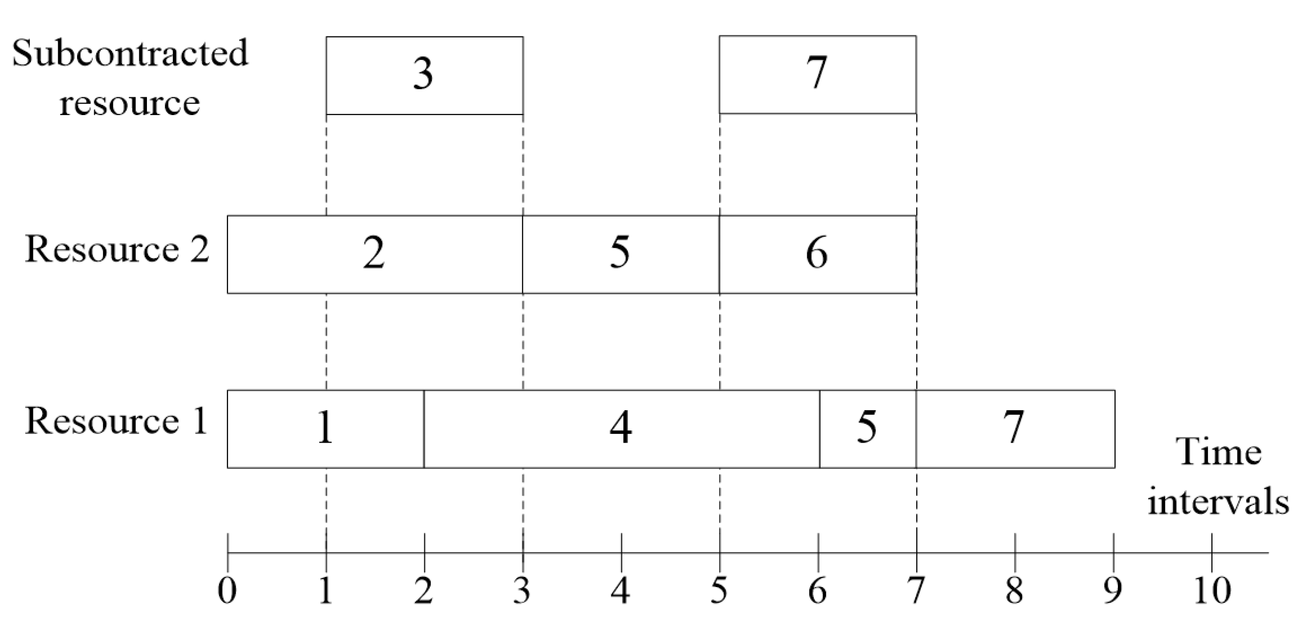
The schedule formed by the V. S. Tanaev method is shown in Figure 3.

We introduce a function ${\mu }_g\left(t\right)$ for subcontracted resources $g=\overline{Q_r,M}$ and define it as follows: ${\mu }_g\left(t\right)=\{\begin{array}{c}1, if S_{k,g}\ne 0, t\in E_k\\ 0, else\end{array}.$ We calculate the subcontracted resources cost according to the formula:

$$Ft=\omega \sum _{t=1}^{e_{\beta +1}}\sum _{g=Q_r}^M{\mu }_g\left(t\right)$$

(14)

For the schedule found by the V. S. Tanaev method, the cost of the subcontracted resources is $Ft=4\omega$.

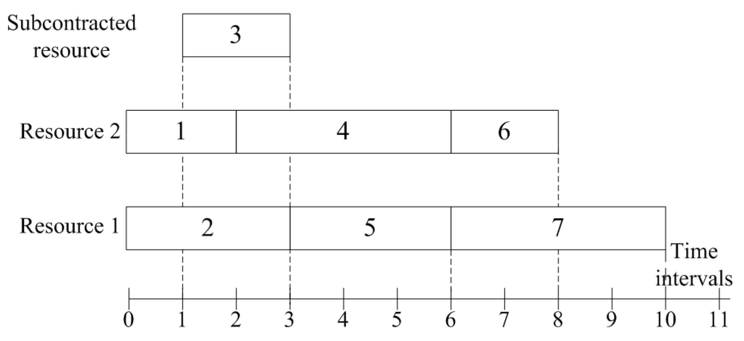
The schedule found is not optimal according to the objective function (8). An example of a more effective schedule satisfying all the requirements (9)–(10) is shown in Figure 4; the subcontracted resources cost is $Ft=2\omega$.

Without loss of generality, let us identify $\omega =100$. Then, $Ft=400$ for the schedule found by the V. C. Tanaev method.

5.3. Method Based on the Commercial Solver Application

We applied a method based on a Lingo solver [22] to the trial scheduling problem. We reduced our mathematical model into a model suitable for linear programming [14].

The decision variables are the following:

• $x_i$ are integer variables indicating the start times of the orders, $i\in P{r}_p$;
• $y_{g,i}$ are binary variables indicating what renewable resource $g$, either own or subcontracted, is allocated to a particular order $i$;
• ${\epsilon }_{i,j}$ are binary variables indicating orders that cannot be executed at the same time because they are to be processed by a single resource $g$.

The mathematical model of this problem applied to a project is described as follows:

$$Kres=\sum _{g\in Rown{\displaystyle \cup }Rsc }\sum _{i\in P{r}_p}{\lambda }_{g,i}\cdot y_{g,i}\to min,$$

(15)

$$\sum _{g\in Rown{\displaystyle \cup }{R}_{sc}}{y}_{g,i}=1, \forall i\in P{r}_p,$$

(16)

$$x_i+d_i\le x_j+ML\cdot \left(1-{\epsilon }_{i,j}\right)+ML\cdot \left(2-y_{g,i}-y_{g,j}\right), \forall \left(i,j\right)\in P{r}_p, \forall g\in Rown{\displaystyle \cup }Rsc,$$

(17)

$$x_j+d_j\le x_i+ML\cdot {\epsilon }_{i,j}+ML\cdot \left(2-y_{g,i}-y_{g,j}\right), \forall \left(i,j\right)\in P{r}_p, \forall g\in Rown{\displaystyle \cup }Rsc,$$

(18)

$$x_{Np}+d_{Np}\le Tdl,$$

(19)

$$Ft=\sum _{g\in Rsc}\sum _{i\in P{r}_p}{\lambda }_{g,i}\cdot y_{g,i}\le Ksc,$$

(20)

$$x_i\ge \tau , \forall i\in P{r}_p,$$

(21)

$$y_{g,i}\in \left\{0,1\right\}, \forall g\in Rown{\displaystyle \cup }Rsc, \forall i\in P{r}_p,$$

(22)

$${\epsilon }_{i,j}\in \left\{0,1\right\}, \forall \left(i,j\right)\in P{r}_p.$$

(23)

For the problem given in Table 1, the following variable values are set:

• The number of projects is $P=1$;
• The cardinality of the $Rown$ set is $\left|Rown\right|=2$;
• The cardinality of the $Rsc$ set is $\left|Rsc\right|=7$, where 7 is the number of orders that can be processed simultaneously;
• The cardinality of the $P{r}_p$ set is $\left|P{r}_p\right|=7$;
• $Ksc=400$ that is limited by the maximum value of the subcontracted resources cost found by the V. S. Tanaev and Y. A. Mezentzev methods;
• $ML=10000$;
• $Tdl=10$ days according to the $d{l}_i$ values from Table 1;
• ${\lambda }_{g,i}=\{\begin{array}{c}1, if g\in Rown\\ 100, if g\in Rsc\end{array}$ $\forall i\in P{r}_p$; we assume that the operation cost should be much lower when processed by the own resource comparing to the subcontracted.

It is defined for this problem that limited non-renewable resources are not considered while they are being introduced in the Formulation (8)–(10).

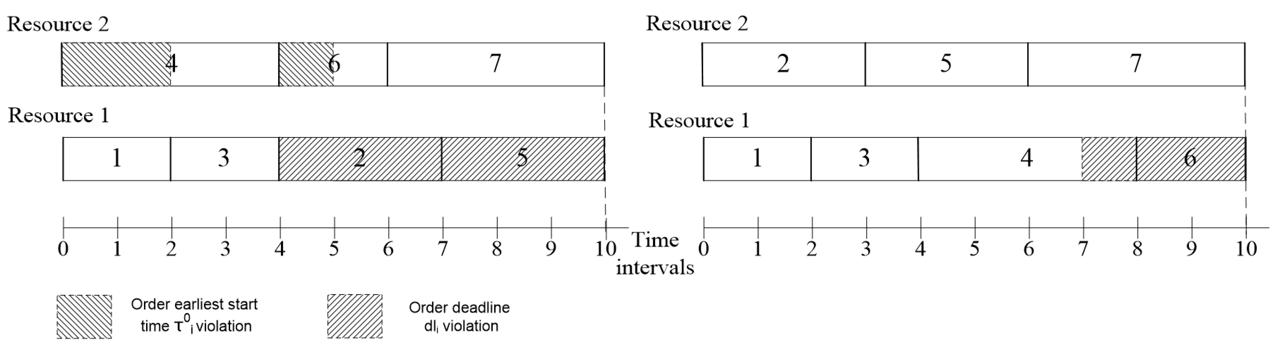
As a result of Lingo execution upon the linear programming problem (15)–(23), a set of alternative optimal schedules was formed providing the same minimum total used resources cost $Kres=7$. Two optimal schedules are presented in Figure 5.

As we can see, the commercial solver was able to reach subcontracting cost $Ft=0$ for the schedules found, but there are violations of the deadline and the orders’ earliest start time.

Thus, application of the commercial solver method leads to violation of the restrictions (9) and (10) of the problem considered.

6. Imitation and Heuristic Method

A key concept of the imitation and heuristic algorithm is integration of processes’ imitation and some heuristic rules to improve the initial schedule. The IH method algorithm is based on an application of a multi-agent resource conversion process (MRCP) model [23]. The MRCP model is intended to describe discrete processes converting input non-renewable resources into output ones using renewable resources, or machines, throughout a given time interval.

An agent of the MRCP model is a decision maker model having formalized knowledge about resources’ allocation using production rules. The MRCP model also includes a logistics agent. The logistics agent controls the current value and lifetime of the non-renewable resources and ensures fulfillment of the restriction (9) by launching the purchase or production process of the non-renewable resource required in case its current volume is decreased to a critical value or the resource’s lifetime is exceeded.

The IH algorithm is a cycle with alternating stages of imitation and application of heuristic rules to improve the schedule. During the imitation stage, the schedule is fed to the MRCP model input, and the model evaluates the subcontracted resources cost according to the Formula (8). During the heuristic stage, the algorithm shifts the start days for the operations, where the subcontracted resources cost exceeds the given threshold. During shifting, the restriction (10) is ensured. The algorithm stops either in the absence of exceeding the threshold of the subcontracted resources cost, or in case a certain number of cycles is reached.

Let us consider the algorithm of the IH method used the MRCP model. The notations are given in Section 3.

The algorithm variables are calculated using the following formulas:

• ${\delta }_{p,i,r}\left(\eta \right)=\left[a;b\right]$ is a time interval where the utilization percentage of the renewable resource $r$ for the operation $i$ is equal to 100%, $U_{p,i,r}^0\left(\eta \right)=100\%$;
• $c_{p,i,r}=b-a$ is the duration of the time interval ${\delta }_{p,i,r}\left(\eta \right)$;
• ${\delta }_{p,i,r}^{-}\left(\eta \right)=\left[\left(a-\left(\eta +1\right)·c_{p,i,r}\right);\left(a-\eta ·c_{p,i,r}\right)\right]$ is the time interval ${\delta }_{p,i,r}\left(\eta \right)$ shifted on the $\left(\eta +1\right)·c_{p,i,r}$ days to the left on the time axis and satisfying the request: $U_{p,i,r}^{-}\left(\eta \right)\ne U_{p,i,r}^0\left(\eta \right)$;
• $U_{p,i,r}^{-}\left(\eta \right)$ is the average utilization of the renewable resource $r$ for the operation $i$ of the project $p$ during the time interval ${\delta }_{p,i,r}^{-}\left(\eta \right)$:

  $$U_{p,i,r}^{-}\left(\eta \right)=\sum _{t=a-\left(\eta +1\right)·c_{p,i,r}}^{a-\eta ·c_{p,i,r}}{U}_{p,t,r}/c_{p,i,r};$$

  (24)
• ${\delta }_{p,i,r}^{+}\left(\eta \right)=\left[\left(b+\eta ·c_{p,i,r}\right);\left(b+\left(\eta +1\right)·c_{p,i,r}\right)\right]$ is the time interval ${\delta }_{p,i,r}\left(\eta \right)$ shifted on the $\left(\eta +1\right)·c_{p,i,r}$ days to the right on the time axis satisfying the request: $U_{p,i,r}^{+}\left(\eta \right)\ne \ne U_{p,i,r}^0\left(\eta \right)$;
• $U_{p,i,r}^{+}\left(\eta \right)$ is the average utilization of the renewable resource $r$ for the operation $i$ of the project $p$ during the time interval ${\delta }_{p,i,r}^{+}\left(\eta \right)$:

  $$U_{p,i,r}^{+}\left(\eta \right)=\sum _{t=b+\eta ·c\left(p,i,r\right)}^{b+\left(\eta +1\right)·c\left(p,i,r\right)}{U}_{p,t,r}/c_{p,i,r}.$$

  (25)

The algorithm of the IH method includes the following stages:

• Conduct experiments with the MRCP model, the input to which are the start dates of operations $x_{p,i}$. Form output model parameters: for each moment $t$ and each project $p$, define a set of operations $O{p}_i\in P{r}_p$ with indexes $i\in \mathsf{{\rm Y}}\left(t,r\right)$ using the subcontract renewable resource $r$ to define the subcontracted resources cost $s{r}^{\prime }{}_{p,i,r}=s{r}_{p,i,r}\cdot q_{p,i,r}$ for each operation; define the utilization $U_{p,t,r}$ for each renewable resource $r$ used for the project $p$; define a function of the current resource volume $Q_{t,v}$ dependence on the time $t$ for each non-renewable resource $v$. Set $p=1$;
• For the project $p$, define the operations with index $i=1,..,N^{\prime }, N^{\prime }\le N_p$, where the subcontracted resources cost $s{r}^{\prime }{}_{p,i,r}$ exceeds the given critical value ${\xi }_{p,i,r}$. If $N^{\prime }\ne 0$, then set $i=1,\eta =1$ and go to Point 3; otherwise, go to Point 6;
• Define the competence of the resource $r$ for the operation $i$ of the project $p$. Highlight a time interval $\left[x_{p,i};x_{p,i}+d_{p,i}\right]$ with a duration $c_{p,i,r}$;
• If the interval ${\delta }_{p,i,r}\left(\eta \right)$ exists, then go to Point 7; otherwise, go to Point 5;
• If $\left(i+1\right)\le N^{\prime }$, then set $i=i+1$ and go to Point 3; otherwise, go to Point 6;
• If $\left(p+1\right)\le P$ then set $p=p+1$ and go to Point 2; otherwise, go to Point 14;
• Calculate the utilizations $U_{p,i,r}^{-}\left(\eta \right)$ and $U_{p,i,r}^{+}\left(\eta \right)$ for the intervals ${\delta }_{p,i,r}^{-}\left(\eta \right)$ and ${\delta }_{p,i,r}^{+}\left(\eta \right)$;
• If $U_{p,i,r}^{-}\left(\eta \right)<U_{p,i,r}^{+}\left(\eta \right),$ then go to Point 9; otherwise, go to Point 10;
• If ${\tau }_{p,i}^0\le \left(x_{p,i}-c_{p,i,r}·\left(\eta +1\right) \right)$–constraint (10) check–then shift the operation’s start as follows:
  • $x_{p,i}=x_{p,i}-c_{p,i,r}·\left(\eta +1\right)$–and go to Point 1; otherwise, go to Point 5;
• If $U_{p,i,r}^{-}\left(\eta \right)>U_{p,i,r}^{+}\left(\eta \right),$ then go to Point 11; otherwise, go to Point 12;
• If $\left(x_{p,i}+c_{p,i,r}·\left(\eta +1\right)\right)\le {\tau }_{p,i}^1$, then shift the operation’s start as follows:
  • $x_{p,i}=x_{p,i}+c_{p,i,r}·\left(\eta +1\right)$–and go to Point 1; otherwise, go to Point 5;
• If $U_{p,i,r}^{-}\left(\eta \right)=U_{p,i,r}^{+}\left(\eta \right)$ and $U_{p,i,r}^{-}\left(\eta \right)\ne U_{p,i,r}^0\left(\eta \right)$, then go to Point 9; otherwise, go to Point 13;
• If $\left(\eta +1\right)\le \mathsf{\Psi }$, then set $\eta =\eta +1$ and go to Point 7; otherwise, go to Point 5;
• The end of the algorithm.

We assess the number of iterations of the IH algorithm.

The number $\mathsf{\Psi }$ of search steps is a parameter of the algorithm. For each step, the algorithm sequentially bypasses all operations of the project portfolio to identify bottlenecks and eliminate them.

The number of operations of the project portfolio is calculated as follows: $N=\sum _{p=1}^P{N}_p$. Thus, the complexity of the proposed IH algorithm linearly depends on the number of operations in the project portfolio according to the formula: $\mathsf{\Psi }·N$. The quality of the schedule found is defined based on the value of the function (8) when restrictions (9)–(10) are fulfilled.

7. Case Study Results

The modified IH scheduling method was implemented in the BPsim software package including the BPsim simulation system and BPsim decision support system [24] with a common database.

The BPsim simulation system is used to develop and simulate the MRCP model of the processes under investigation. The system supports graphical MRCP notation, where a user can identify the types of nodes, i.e., operations and agents, logical links between them, and list the available non-renewable and renewable resources.

The following parameters can be assigned to each operation: the duration, start condition, amount of non-renewable and renewable resources required to complete the operation, and amount of produced non-renewable resources. To each agent, the behavior rules can be described in a form of if-then rules and assigned. The agents can affect the amount of resources and operations’ start conditions.

The BPsim decision support system includes decision search diagrams based on the same resources used to build the simulation model. Development of the diagrams is based on the UML sequence diagrams [25] and Transact-SQL database management language [26]. The decision search diagrams are used to provide a visual comparison for multiple alternative decisions utilizing implemented user rules. The diagrams were applied to implement the algorithm of the IH scheduling method.

A case study was used to assess the subcontracted resources cost depending on the current schedule of 10 projects with 35 operations in a project company. The company has its own renewable resources, i.e., a staff of eight people with different skills (competencies). The following competencies of the staff were defined: documentation design (three people), carrying out an installation work (four people), and material supply (one person). The non-renewable resources of the company are the construction objects. The operation duration varied from 6 days to 90 days depending on the type of operation. The scheduling time interval was 430 days.

Following the proposed IH scheduling method, a simulation model was developed in the BPsim simulation system. The model’s inputs are the labor costs and the agreed start dates for each operation, as well as the schedule. Assessment of the subcontracted resources cost was produced by the model.

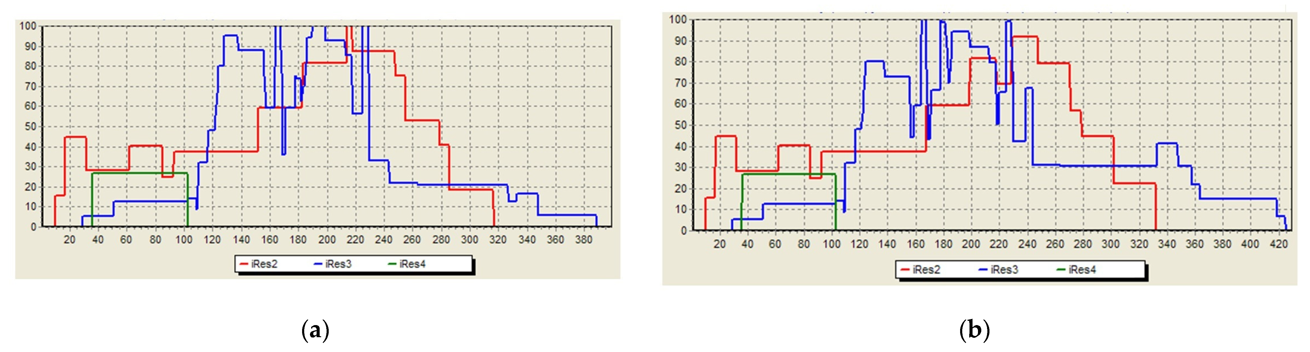
For the initial schedule, the model outcome is presented in Figure 6a. For the schedule provided by the IH method, the model outcome is presented in Figure 6b.

The figures contain the percentage utilization of the three own resources with different competence marked with the red, blue, and green lines. When the blue and red resources utilization reaches the 100% level, it means the subcontracted resources with the matched competence are used during this time. The green resource utilization does not exceed 30% in both figures, so subcontracted resources with the same competence are not required.

The initial and the final schedules coincide up to 110 days due to the low resource utilization at the initial schedule during these days. Therefore, the IH algorithm has not shifted the operations’ start day during the first 110 days in the final schedule.

Table 6. Subcontracted resources’ cost allocation for the initial schedule.

Operation Name	Project 1	Project 3	Project 4	Project 5	Project 9
Development of technical specification in man per day (m/d)	3.9 m/d			1.68 m/d
Installation and commissioning work (telemechanics) in m/d			2.45 m/d
Installation and commissioning work (energy accounting) in m/d		11.54 m/d			8.53 m/d
Installation and commissioning work (telecommunications) in m/d			13.88 m/d
Overall subcontract cost of the project in man per day	3.9 m/d	11.54 m/d	16.33 m/d	1.68 m/d	8.53 m/d
Overall subcontract cost of the project in rubles	10 249	95 990	65 998	6 746	70 953
Overall subcontract cost of the portfolio in m/d	41.98 man per day
Overall subcontract cost of the portfolio in rubles	249,936 rubles

contains allocation of the subcontracted resources’ cost in rubles and man per day (m/d) on the project’s operations for the initial schedule.

For the initial schedule, the subcontracted resources are required for the projects 1, 3, 4, 5, and 9. The IH method allowed us to highlight several operations with a subcontracted resources cost exceeding the critical value equal to 60,000 rubles. The ones are installation works for projects 3 and 9 (95,990 and 70,953 rubles accordingly), and all operations for project 4 (65,998 rubles).

Table 7. Subcontracted resources’ cost allocation for the schedule provided by the IH method.

Operation Name	Project 1	Project 3	Project 4	Project 5	Project 9
Development of technical specification in man per day (m/d)				1.68 m/d
Installation and commissioning work (energy accounting) in m/d					4.04 m/d
Installation and commissioning work (telecommunications) in m/d			2 m/d
Customer training in m/d	0.36 m/d	0.46 m/d
Overall subcontract cost of the project in man per day	0.36 m/d	0.46 m/d	2 m/d	1.68 m/d	4.04 m/d
Overall subcontract cost of the project in rubles	946	3826	8330	6746	33,605
Overall subcontract cost of the portfolio in m/d	8.54 man per day
Overall subcontract cost of the portfolio in rubles	53,453 rubles

contains allocation of the subcontracted resources’ cost in rubles and m/d on the project’s operations for the schedule provided by the IH method.

The IH method is proposed resource allocation and shifting of the operations’ start date within a given timeframe. Although, the makespan of the found schedule was increased compared with the initial schedule, all operations and project deadlines were met.

It should be noted that the objective function considered is related to minimization of the subcontracted resources’ cost while meeting restrictions. As a result, the subcontracted resources’ cost of the schedule found was reduced compared with the initial schedule in terms of man per day from 42 m/d to 9 m/d and in terms of rubles from 249,936 rubles to 53,453 rubles for half a year, i.e., more than four times for both outcomes.

8. Discussions

The results of the scheduling methods’ comparison are shown in

Table 8. The results of the scheduling method comparison.

Method	Subcontracted Resources Accounting	Subcontracted Cost Optimization, (8)	Non-Renewable Resources Accounting, (9)	Deadlines Accounting (10)	Earliest Start Time Accounting (10)	Multi-Objective Optimization
Y. A. Mezentsev method [4]	No	No	No	No	Yes	No
V. S. Tanaev method [5]	Yes	No	No	Yes	No	No
Lingo based method [14]	Yes	Yes	No	No	No	No
Agent-based method [7]	Yes	No	Yes	Yes	Yes	Yes
GA-based method [9]	No	No	Yes	No	No	No
OptQuest based method [11]	No	No	No	Yes	No	Yes
Plant Simulation method [13]	No	No	Yes	Yes	No	Yes
IH method	Yes	Yes	Yes	Yes	Yes	No

.

As we can see from Table 8, all the methods have disadvantages when solving the project scheduling problem considered. The problem has the following features: search for a solution with the minimum subcontracted resources cost, large dimension of the search space, presence of the operations start time interval, and allocation of renewable and non-renewable resources with a restricted non-renewable resources lifetime. These features restrain the application of the scheduling theory methods considered. The Y. A. Mezentsev and V. S. Tanaev methods solve the scheduling problem while minimizing the makespan by tight packing of operations in compliance with part of the restrictions. However, the issues of attracting and optimizing the subcontracted resources cost are not given due attention. The Lingo-based method deals with subcontracting cost optimization, but the schedule found does not satisfy any constraint. The agent-based method lacks subcontracted resource optimization but considers all the restrictions, including the non-renewable resources one. The GA-based method and the commercial solver-based methods, OptQuest and GA of the Plant Simulation, do not consider the subcontracted resources and orders’ earliest start times while the GA-based method accounts for restricted non-renewable resources.

Application of simulation multi-agent modeling with heuristic rules of the resource’s allocation allows us to consider all features of the scheduling problem except multi-objective optimization. The HI method optimizes the subcontracted resources cost taking into account restricted renewable and non-renewable resources and orders’ earliest start times. At the same time, a project duration may increase wherein the orders deadlines are met.

For the scheduling problem with 35 operations, eight renewable resources and one type of non-renewable resource, the running time of the HI algorithm is estimated at 6 min. This time is comparable to the running time of the methods based on agents, OptQuest, and Plant Simulation application. The HI algorithm running time is much more than the one of the methods proposed by Y. A. Mezentsev and V. S. Tanaev as well as the Lingo- and GA-based ones, estimated at tens of seconds. It should be noted that the search time for the simulation-based methods is always more than the search time for the methods based on the optimization algorithms. When simulating, a time for conducting one experiment varies from a few seconds to several minutes depending on the model dimension and simulation tool used. In case of solving the optimization problem, it is necessary to search for solutions in a search space while the alternative solution is estimated by conducting an experiment with the model; therefore, the total search time increases to tens or even hundreds of minutes. Nevertheless, simulation-based methods have the advantage of being able to determine the objective function and the constraints required without a reduction to a specific mathematical model used in optimization algorithms.

We also applied the HI algorithm to the scheduling problem with a large data set. A construction holding was considered with 302 building operations, 119 renewable resources or construction machinery, and 161 types of non-renewable resources or construction material. The detailed holding description is given in [27]. For the problem with a large data set, the running time of the HI algorithm is estimated at one hour and 38 min. The given duration of the algorithm operation is rather long compared to the obtained one for the small dimension problem but is acceptable for decision making that is not in real time.

9. Conclusions

The scheduling problem was formulated with the objective function of minimization of the subcontracted resources cost, presence of restrictions on non-renewable resources, and operations’ earliest start time and due dates. Analysis of the different scheduling methods based on the scheduling theory, optimization algorithms, and agent-based simulation was conducted. The analysis revealed factors preventing application of the methods to the problem under consideration. The factors include lack of a search for the optimal allocation of renewable resources on operations in terms of minimizing the subcontracted resources’ cost and lack of accounting for limited non-renewable resources. The given factors indicate the relevance of the development of the hybrid scheduling method based on integration of simulation and heuristic modeling.

The IH method algorithm was developed based on the multi-agent simulation model of the resource’s allocation with operations performing and heuristic rules of the operations start days shifting. The IH method is used to search the schedule that meets the time and resources restrictions and has a minimum subcontracted resources cost.

A case study was conducted to assess the subcontracted resources cost for the real scheduling problem of a project company. Application of the IH method allowed us to compose a schedule that reduced the company’s waste on subcontracted resources by more than four-fold for half a year compared with the schedule provided by decision makers based on their knowledge and experience.

Comparison of the IH method and the other scheduling heuristic methods was performed. The conditions were identified, under which the new IH method is more effective than the other ones. The conditions include a focus on optimizing the project portfolio cost with a fixed portfolio duration. In future, the authors plan to refine the IH method for solving the multicriteria problem of finding a schedule that is optimal in terms of the makespan and the renewable resources cost.

References

- Clark, C.E. The PERT model for distribution of an activity time. Oper. Res. 1962, 10, 405–406. [Google Scholar] [CrossRef] [Green Version]
- Kannan, R. Graphical evaluation and review technique (GERT): The panorama in the computation and visualization of network-based project management. Adv. Secur. Comput. Internet Serv. Appl. 2014, 9, 165–179. [Google Scholar] [CrossRef]
- Gimadi, E.K.; Goncharov, E.N.; Mishin, D.V. On some implementations of solving the resource constrained project scheduling problems. Yugosl. J. Oper. Res. 2019, 29, 31–42. [Google Scholar] [CrossRef] [Green Version]
- Mezentsev, Y.A.; Estraykh, I.V.; Chubko, N.Y. Implementation of an efficient parametric algorithm for optimal scheduling on parallel machines with release dates. J. Phys. Conf. Ser. Inf. Technol. Bus. Ind. 2019, 1333, 022002. [Google Scholar] [CrossRef]
- Tanaev, V.S.; Shkurba, V.V. Introduction to the Scheduling Theory; Science: Moscow, Russia, 1975. [Google Scholar]
- Guizzi, G.; Vespoli, S.; Grassi, A.; Carmela Santillo, L. Simulation-based performance assessment of a new job-shop dispatching rule for the semi-heterarchical industry 4.0 architecture. In Proceedings of the 2020 Winter Simulation Conference (WSC), Orlando, FL, USA, 14–18 December 2020; pp. 1664–1675. [Google Scholar] [CrossRef]
- Skobelev, P.; Zhilyaev, A.; Larukhin, V.; Grachev, S.; Simonova, E. Ontology-based open multi-agent systems for adaptive resource management. In Proceedings of the 12th International Conference on Agents and Artificial Intelligence, Valletta, Malta, 22–24 February 2020; pp. 127–135. [Google Scholar] [CrossRef]
- Goncharov, E.; Leonov, V. Genetic algorithm for the resource-constrained project scheduling problem. Autom. Remote Control 2017, 78, 1101–1114. [Google Scholar] [CrossRef]
- Xie, L.; Chen, Y.; Chang, R. Scheduling optimization of prefabricated construction projects by genetic algorithm. Appl. Sci. 2021, 11, 5531. [Google Scholar] [CrossRef]
- Guizzi, G.; Revetria, R.; Vanacore, G.; Vespoli, S. On the open job-shop scheduling problem: A decentralized multi-agent approach for the manufacturing system performance optimization. In Proceedings of the 12th CIRP Conference on Intelligent Computation in Manufacturing Engineering, Gulf of Naples, Italy, 18–20 July 2018; pp. 192–197. [Google Scholar] [CrossRef]
- Alvandi, S. Energy efficiency improvement through optimal batch sizing in job shop. Mod. Appl. Sci. 2020, 14, 6–19. [Google Scholar] [CrossRef]
- Ištoković, D.; Perinić, M.; Doboviček, S.; Bazina, T. Simulation framework for determining the order and size of the product batches in the flow shop: A case study. Adv. Prod. Eng. Manag. 2019, 14, 166–176. [Google Scholar] [CrossRef] [Green Version]
- Yu, H.; Han, S.; Yang, D.; Wang, Z.; Feng, W. Job shop scheduling based on digital twin technology: A survey and an intelligent platform. Hindawi Complex. 2021, 1–12. [Google Scholar] [CrossRef]
- Biruk, S.; Jaśkowski, P.; Czarnigowska, A. Minimizing project cost by integrating subcontractor selection decisions with scheduling. IOP Conf. Ser. Mater. Sci. Eng. 2017, 245, 072007. [Google Scholar] [CrossRef]
- Pinedo, M.L. Scheduling: Theory, Algorithms, and Systems Development; Springer: Berlin/Heidelberg, Germany, 2008. [Google Scholar] [CrossRef]
- Wooldridge, M.; Jennings, N. Intelligent agent: Theory and practice. Knowl. Eng. Rev. 1995, 10, 115–152. [Google Scholar] [CrossRef] [Green Version]
- Goldberg, D.; Holland, J.H. Genetic algorithms and machine learning. Mach. Learn. 1988, 3, 95–99. [Google Scholar] [CrossRef]
- OptQuest, the Official Web Site. Available online: https://www.opttek.com/products/optquest/ (accessed on 19 August 2021).
- Anylogic Simulation Software, the Official Web Site. Available online: https://www.anylogic.com/ (accessed on 19 August 2021).
- Optimize Production Logistics & Material Flow. Siemens Tecnomatix Plant Simulation, the Official Web Site. Available online: https://www.plm.automation.siemens.com/global/en/products/tecnomatix/logistics-material-flow-simulation.html (accessed on 19 August 2021).
- Antonova, A.S.; Aksyonov, K.A. Analysis of the methods for accounting the renewable and non-renewable resources in scheduling. In Proceedings of the 7th ITTCS International Young Scientists Conference on Information Technology, Telecommunications and Control Systems, Innopolis, Russia, 17–18 December 2020. [Google Scholar] [CrossRef]
- LINGO 19.0—Optimization Modeling Software for Linear, Nonlinear, and Integer Programming. Available online: https://www.lindo.com/index.php/products/lingo-and-optimization-modeling (accessed on 19 August 2021).
- Aksyonov, K.; Bykov, E.; Aksyonova, O.; Goncharova, N.; Nevolina, A. The architecture of the multi-agent resource conversion processes. In Proceedings of the UKSim 11th European Modelling Symposium on Mathematical Modelling and Computer Simulation, Manchester, UK, 20–21 November 2017; pp. 61–64. [Google Scholar] [CrossRef]
- Aksyonov, K.; Aksyonova, O.; Antonova, A.; Aksyonova, E.; Ziomkovskaya, P. Development of cloud-based microservices to decision support system. In Proceedings of the International Conference on Open Source Systems, OSS 2020, Innopolis, Russia, 12–14 May 2020; pp. 87–97. [Google Scholar] [CrossRef]
- The official UML Web Site. Available online: http://www.uml.org (accessed on 19 August 2021).
- SQL Server language reference. Available online: https://docs.microsoft.com/en-us/previous-versions/sql/sql-server-2005/ms189826(v=sql.90) (accessed on 19 August 2021).
- Aksyonov, K.A.; Bykov, E.A.; Aksyonova, O.P.; Wang, K. Application of BPsim.DSS system for decision support in a construction corporation. Appl. Mech. Mater. 2013, 256–259, 2886–2889. [Google Scholar] [CrossRef]
Figure 1.
Schedules received by the Y. A. Mezentsev method with the minimum makespan.
Figure 2.
Time intervals of orders’ processing for the trial problem.
Figure 3.
Schedule provided by the V. S. Tanaev method.
Figure 4.
Schedule with the most effective resource allocation.
Figure 5.
Two optimal schedules provided by the commercial solver.
Figure 6.
Percentage utilization U of own resources iRes performing the project’s portfolio depending on time: (a) Initial schedule; (b) Schedule provided by the IH method. Here, iRes2 is a resource with the documentation design competence, iRes3 is a resource with the competence to carry out installation works, and iRes4 is a resource with material supply competence.