Article

Inferring HIV Transmission Network Determinants Using Agent-Based Models Calibrated to Multi-Data Sources

by
David Niyukuri
1,2,*,
Trust Chibawara
1,
Peter Suwirakwenda Nyasulu
2,3 and
Wim Delva
1,2,4,5,6
1
Division of Epidemiology & Biostatistics, Faculty of Medicine and Health Sciences, Stellenbosch University, Cape Town 7505, South Africa
2
The Department of Science and Technology-National Research Foundation (DST-NRF)/South African Centre of Excellence in Epidemiological Modelling and Analysis (SACEMA), Stellenbosch University, Stellenbosch 7600, South Africa
3
Division of Epidemiology & Biostatistics, School of Public Health, Faculty of Health, University of the Witwatersrand, Johannesburg 2000, South Africa
4
Center for Statistics, I-BioStat, Hasselt University, 3590 Diepenbeek, Belgium
5
International Centre for Reproductive Health, Ghent University, 9000 Ghent, Belgium
6
Rega Institute for Medical Research, KU Leuven, 3000 Leuven, Belgium
*
Author to whom correspondence should be addressed.
Submission received: 2 September 2021 / Revised: 29 September 2021 / Accepted: 9 October 2021 / Published: 20 October 2021
(This article belongs to the Special Issue Mathematical Biology: Modeling, Analysis, and Simulations)

Abstract

:
(1) Background: Calibration of Simpact Cyan can help to improve estimates related to the transmission dynamics of the Human Immunodeficiency Virus (HIV). Age-mixing patterns in sexual partnerships, onward transmissions, and temporal trends of HIV incidence are determinants which can inform the design of efficient prevention, and linkage-to-care programs. Using an agent-based model (ABM) simulation tool, we investigated, through a simulation study, if estimates of these determinants can be obtained with high accuracy by combining summary features from different data sources. (2) Methods: With specific parameters, we generated the benchmark data, and calibrated the default model in three scenarios based on summary features for comparison. For calibration, we used Latin Hypercube Sampling approach to generate parameter values, and Approximation Bayesian Computation to choose the best fitting ones. In all calibration scenarios the mean square root error was used as a measure to depict the estimates accuracy. (3) Results: The accuracy measure showed relatively no difference between the three scenarios. Moreover, we found that in all scenarios, age and gender strata incidence trends were poorly estimated. (4) Conclusions: Using synthetic benchmarks, we showed that it is possible to infer HIV transmission dynamics using an ABM of HIV transmission. Our results suggest that any type of summary feature provides adequate information to estimate HIV transmission network determinants. However, it is advisable to check the level of accuracy of the estimates of interest using benchmark data.

1. Background

The Human Immunodeficiency Virus (HIV) infection remains a major public health concern in sub-Saharan Africa (SSA). The vast majority of new HIV infections are caused by unprotected sexual intercourse [1]. Thus, sexual transmissions are believed to be the main driver of the epidemic in that part of the world [2,3]. High-risk sexual behaviour of individuals, such as having a large number of concurrent and lifetime sexual partners, and a high frequency of unprotected sex increases the risk of acquiring HIV infection [2,4,5,6,7]. Thus, for HIV and other sexually transmitted diseases, individual behaviours affect the transmission dynamics [8]. Our understanding of patterns of age-related sexual partner choices at population level known as age-mixing patterns [9] can help to undertake behaviour change interventions to prevent HIV transmission.
Temporal trends of HIV incidence [10], help us to see the impact of interventions on reducing new infections among populations [11,12]. Given the type and quality of ongoing HIV interventions, new infections may (or may not) produce secondary HIV transmissions. Thus, temporal trends of incidence alone do not give a full picture of the impact of interventions. Given a time interval, in a population where one infected individual generate only one secondary infection, if many of them are infected in that population, the number of new infections may be the same as when few infected individuals generate many secondary infections. Hence, we need also to estimate the distribution of onward HIV transmission.
Therefore, from a public health point of view, estimating age-mixing patterns in sexual partnerships, the distribution of onward HIV transmission, and temporal trends of HIV incidence, are important to inform the design of more effective and efficient HIV prevention and linkage-to-care programs.
Most of traditional HIV studies look at prevalence, incidence, distribution of the infection in different populations, and the risk of acquiring the infection. These types of studies use mostly epidemiological data, clinical, and sexual behavioural survey data [2,13]. Either models are fitted to these data [14,15], or statistical analysis is performed on them [3,13,15,16]. However, if we want to understand some key features of HIV infection, such as mixing between different groups of the populations of interest, the rapidity of viral spread within populations, transmission clusters and where new infections occur, and the transmission of drug resistance [17,18], we concur with the idea of undertaking phylogenetic analysis which uses viral sequence data. As HIV is transmitted across a sexual network, the structure and dynamics of the sexual network shape the evolution of the virus population [19]. The analysis of HIV phylogenetic trees (constructed from HIV sequences sampled from infected individuals) has the ability to determine estimates of some transmission network determinants of realised sexual networks [20].
The main output of a phylogenetic analysis is a phylogenetic tree, which is a diagram that represents evolutionary relationships among organisms or genes [21]. If constructed from viral sequences of infected individuals, it holds information about the structure of a sexual network [19], and the transmission dynamics [22,23]. The shape of a phylogenetic tree consists of two properties, the topology (particular branching pattern for a tree), and the branch lengths [24]. Thus, some topological features from a phylogenetic tree, such as the Colless imbalance and “ladder length”, are properties that have been identified to distinguish different transmission patterns [25]. In a “super-spreader” pattern, most infected people produce no or one onward transmission, while a small fraction produce a high number of onward transmissions [25]. In chain-like transmission, the vast majority of infected people produce exactly one onward transmission, while a few exceptions produce two or three onward transmissions. In a homogeneous transmission pattern, onward transmissions are Poisson-distributed. Thus, summary features from phylogenetic tree data were used to calibrate modelling framework and estimate HIV transmission networks [26], and sexual contact networks [19]. Despite some challenges related to phylogenetic analysis assumptions [17], viral sequence data were used to infer temporal trends of HIV incidence [22,27,28], as well as the age difference in HIV transmission clusters [18], and other important epidemiological parameters such as the basic reproductive number R 0  [29].
The estimates of the abovementioned HIV transmission network determinants (age-mixing patterns in sexual partnership, HIV temporal trend of incidence, and onward transmission) give an overview of the extent of age-mixing patterns in the sexual network, HIV transmission dynamics, and the effect of interventions. These estimates may be elusive or difficult to estimate, and we often rely on models which we fit to existing data. Fitting models to empirical data is known as calibration, and it entails searching the best fit values for the models’ parameters which can generate the data, given the observed summary features (known as target summary statistics) from observed data. We used Simpact Cyan [30], an integrated modelling framework which is an agent-based model (ABM) used to run a simulation study from which we explore its calibration with regard to estimation of determinants of the HIV transmission network. Thus, since this study is a simulation study, the observed data would be the benchmark data generated with a known vector of parameter values. This has been elaborated in detail in the methodology section.
Some authors argued that combining different data sources such as epidemiological data, social network data, phylogenetic tree data, and many more, has the potential to improve epidemic estimates, and thereafter advance public health interventions [31,32,33]. Therefore, we hypothesised that combining summary features from epidemiological and behavioural data, and phylogenetic tree data to calibrate the Simpact Cyan model [30] can improve estimates for age-mixing patterns in sexual partnerships, the distribution of onward transmissions, and the temporal trends of HIV incidence.
Simpact Cyan, being an HIV simulation tool, can therefore be applied and utilised as a modelling framework which simulates sexual dynamic networks, HIV transmission, and viral evolution across transmission networks. It has potential to help us understand some parts of complexity of sexual partnerships across sexual networks. Furthermore, it helps to advance methodological studies related to the use of HIV viral data that aim to understand HIV transmission networks [34]. This simulation study opens research pathways for calibration studies which would use Simpact Cyan, focusing on HIV inferences by shedding light on key considerations such as those from phylogenetic trees for summary features and parameter estimation. Thus, with this simulation study, we wanted to see if, by using synthetic benchmarks data, we can infer HIV transmission network determinants using an agent-based model simulation tool for HIV infection transmission.

2. Methods

2.1. Simulation Tool: Simpact Cyan

In this simulation study, we used Simpact Cyan [30], a modelling framework which simulates demographic events (birth and deaths), sexual dynamic networks, HIV transmission across sexual networks, and viral evolution across transmission networks. The core of the simulation tool is based on agent-based models, and the interactions of agents for sexual partnerships and HIV transmission, together with other events, are defined by hazard functions. These hazard functions are mathematical quantities which give the rate at which an event such as establishing or dissolving a sexual partnership, HIV transmission, birth, or death occurs. With fine-grained detail of agent-based models, we were able to add another component to simulate viral evolutionary dynamics above the transmission network. This allowed for the use of multiple data sources including sequence data in our simulation and analysis. More details of the components of the simulation tool are described in the Appendix A. The details of the Simpact Cyan simulation model are also given in the Appendix A, which is a part of the paper’s supporting information of the paper [34].

2.2. Simulation of HIV Epidemic

We simulated sexual partnership dynamics, HIV transmission, and viral evolution across transmission networks using Simpact Cyan [30,35]. The simulation time was 40 years (0 to 40 years). Due to the phylogenetic component of the simulation (the age of the root sequence we used), we considered calendar time, and the simulation time became 40 years between 1977 and 2017. We defined an initial population of men (5000) and women (5000). During the simulation, a sexual partnership was set to start 10 years earlier before the introduction of HIV in the population to allow equilibrium of partnership establishment/dissolution events. To initiate HIV transmission, 10 individuals aged randomly between 20 and 50 years were seeded with being HIV positive allowing the HIV model to run its course. Thus, HIV infection was introduced in 1987, and subsequent transmissions occurred up to 2017.
The simulation framework contains different hazard functions that capture the dynamic of sexual partnerships, HIV transmission, and ART intervention, among others. These functions were established based on different assumptions to ensure the simulated dynamics of HIV epidemic can be a proxy, hence depicting the real world situation. For instance, HIV transmissions are assumed to occur as a function of partner HIV status, viral load levels, antiretroviral therapy (ART) intervention and follow-up of the HIV positive partner. The gradual treatment eligibility based on the Cluster of Differentiation 4 (CD4) protein counts as implemented in the real world [36,37], was considered in the epidemic simulation. We considered 100, 150, 200, 350, 500, 700 CD4 counts for 23, 25, 28, 33, 36, 39 simulation years, respectively.
At the 40 years of simulation time point (2017 in calendar time), the simulated HIV epidemic exhibited different trends of prevalence between women and men. Younger women had higher prevalence compared to men of the same age groups as we can see in Figure 1. Between 39 and 40 years of simulation time (2016 and 2017 in calendar time), younger women (below 25 years) had higher incidence compared to men of the same age group as we can see in Figure 2. Thus, the simulated epidemic mimics commonly observed trends in generalised HIV epidemic settings in SSA [38,39,40].
The viral evolution across the transmission network was simulated using a transmission tree built from the transmission network, to simulate viral sequences (each per individual) with a general time-reversible ( G T R ) + Γ model in Seq-Gen with a seed sequence [41]. The main advantage of this integrated simulation framework is that it enables estimation/computation of known measurements associated to the HIV epidemic, which may be elusive or hard to estimate in real life.
Key assumptions for HIV simulation and molecular evolution of the simulation model were provided. For HIV simulation, we had considerations on demographics, sexual partnerships, HIV transmission, ART interventions, and disease progression. For molecular evolution of the virus, we considered population-level variation of viral sequences with GTR substitutions of nucleotides. More details on these assumptions mentioned above are given in the Appendix A (Table A2 and Table A3), which describes in more detail the simulation model and its components.
To generate benchmark data of reference, we assigned values to 13 selected parameters which are some of the known parameters to have direct effects on sexual partnerships, and HIV transmission; more details for those parameters can be seen in the Appendix B. With those parameter values, we ran the integrated simulation framework 1120 times in order to take into account stochasticity. The simulation framework with values of the selected parameters was considered a “master model”. From that model, we computed the measurements of interest in our study which were parameters for age-mixing patterns in sexual partnerships, temporal trends of HIV incidence, and the distribution of onward transmissions. We also computed two types of summary features: epidemiological and behavioural summary features, and phylogenetic tree summary features. These summary features were used to calibrate the default integrated simulation framework in three scenarios: (i) with epidemiological and behavioural features, (ii) with phylogenetic tree features, and (iii) with combined features.
In our simulation, for a man i with n partnerships, there were n age gap preferences, this gave clustered data regarding age gaps. The equation below (1) explains the variation of the man’s age gap preference for his women partners with a linear mixed random-effect model [42]:
y i j = β 0 x i j + β 1 + b i + ϵ i j
where y i j represents the age gap preference of woman j in sexual partnership with man i, and x i j was the predictor which was the age of the man i. The parameters β 0 and β 1 represent the fixed effects, while b i parameters represent the random effects.
In our calibration exercise, we had two types of parameters to estimate age-mixing patterns in sexual partnerships; one was a set of descriptive parameters for age difference between a male and his female partners, namely the average age difference (AAD) across sexual partnerships, and the standard deviation of the age difference (SDAD). We also had parameters from the linear mixed random-effect model (LMM) given by Equation (1), which was fitted to the clustering data of age gap preference for men. Fitting the LMM to the data using the R package l m e 4 [43], we obtained other age-mixing parameters: the within-subject standard deviation of age differences (WSD), the average variation of age gap within the clusters of men’s age gaps; the between-subject standard deviation (BSD), the average variation of age gap between the clusters of men’s age gaps; the slope and intercept which show the overall population level trend of age gap preference.
For distribution of onward transmissions, we computed the mean, median, and standard deviation of the number of infected individuals, secondary generated by an infected individual who died between 35 and 40 years simulation time.
In addition for temporal trends (35–40 years of simulation time) of HIV incidence, we computed incidence values per year per age group (15–24, 25–29, 30–34, 35–39, 40–44 and 45–49 years) among men and women. We considered one year interval for incidence between 35 and 40 years of simulation time.
The calibration process entails the use of summary features (from benchmark data) which are also known as target statistics—which are always considered to be measurable from real data, and calibrate the default simulation framework (Simpact Cyan). Given the benchmark summary features (target statistics) and a parameter space where we can search parameter values, the calibration process aimed to find best guess of parameter values which produce summary features which are close to those from benchmark data. We then use these parameter values to run the simulation framework, and compute the parameters for age-mixing patterns in sexual partnerships, temporal trends in HIV incidence, and the distribution of onward transmissions at a certain level of accuracy when we can compare them to what we obtained in the benchmark data.
All the above mentioned transmission network determinants and summary features were computed from data sampled between 35 and 40 years of simulation time, which was 2012 and 2017 in calendar time.

2.3. Selected Parameters for Calibration

Simpact Cyan has many parameters, as we can see in its documentation [35]. Details about all events, associated settings, and their parameters are explained in the documentation. In our calibration exercise, we selected parameters of sexual partnership events with related settings, sexual partnership dissolution events, and HIV transmission events. More details of these parameters can be found in the Appendix A, where we described the Simpact Cyan simulation model, in the Appendix A.2 for events’ hazard functions and associated settings.

2.4. Selected Summary Features

The summary features were chosen with regard to how we believe they can capture information of the transmission network determinants (age-mixing patterns in transmission, onward transmission, and temporal trends of incidence). The benchmark values for epidemiological and behavioural features were computed from demographic, sexual behavioural, HIV epidemic, and intervention benchmark data. The phylogenetic tree features were computed from a phylogenetic tree built from sequence data. The first calibration process was conducted by considering only features from epi-behavioural data; the second was conducted with phylogenetic features; and the third was conducted with combined features. More details about summary features are given in the Appendix B.
The following summary features were selected for epidemiological and sexual behaviour data: (i) population growth rate between 35 and 40 years of simulation time; (ii) HIV infection point prevalence (40 years of simulation time) for men and women in different age groups (15–24 years, 25–29 years, 30–34 years, 35–39 years, 40–44 years, and 45–49 years) at 40 years of simulation time (end of simulation); (iii) HIV infection incidence (39–40 years of simulation time) for men and women in different age groups (15–24 years, 25–29 years, 30–34 years, 35–39 years, 40–44 years, and 45–49 years); (iv) prevalence of concurrent partnerships (39.5–40 years of simulation time); (v) relationship per person per year (35–40 years of simulation time); (vi) mean, median, and standard deviation of age difference between infected individuals (35–40 years of simulation time); (vii) anti-retroviral treatment coverage (from 33 to 40 years of simulation time); and (viii) viral load suppression at 40 years of simulation time for individuals with ≥15 years but <50 years.
On the other hand, we derived the following summary features from phylogenetic tree data: (i) mean, median, and standard deviation of of internal nodes; (ii) mean, median, and standard deviation of tree height; (iii) Colless and Sackin indexes; (iv) minimum, maximum, mean, median, standard deviation, 1st and 3rd quantiles of branch length; (v) mean, median, standard deviation of tips depths; (vi) mean, median, standard deviation of of nodes depth; and (vii) maximum height. Whenever phylogenetic data were used, the calibration process was conducted with summary features computed at 100% of sampling coverage in a scenario where we assumed that missing sequences were missing completely at random (MCAR).
Since, the master model was executed 1120 times, to summarise the summary features to be used during calibration, we considered mean values for each target statistic. We did the same regarding mean values for parameters of the HIV transmission network determinants.

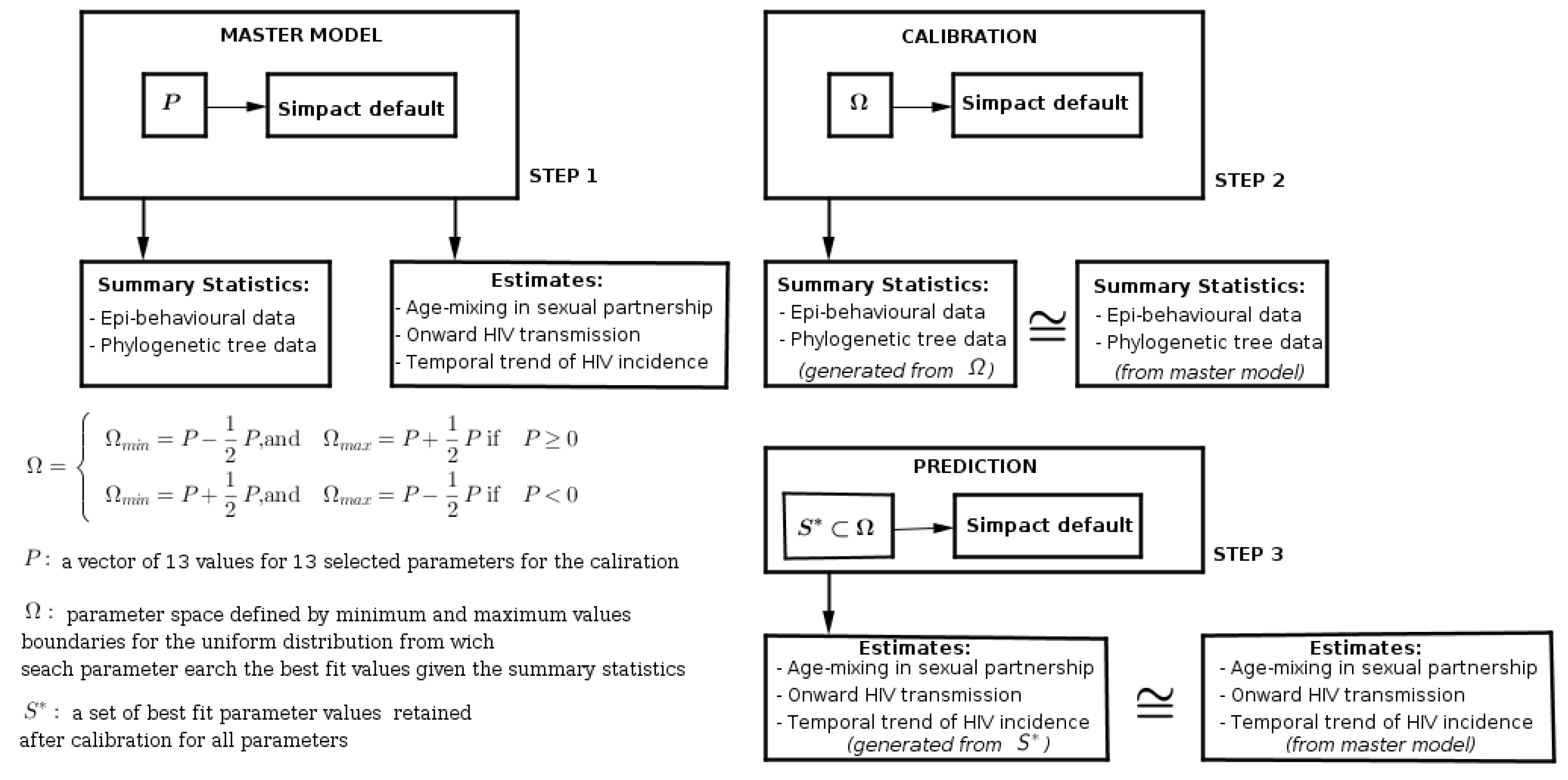
2.5. Calibration Scheme

The calibration process was performed using Latin Hypercube Sampling (LHS) [44,45], a technique used to generate parameter(s) values in given parameter(s) space(s), together with the rejection method of Approximation Bayesian Computation (ABC) [46], an approach used to choose the best candidate of parameter(s) values given the summary features from benchmark data. Because we had to retain only 30% best fit parameter values with ABC calibration, we had to be able to run the model after calibration with 1120 parameter combinations; thus, we had to generate 3752 parameter values. With the Latin Hypercube sampling technique, we set 3752 sampling cells for parameter space for each parameter among the 13 parameters. Each parameter had 3752 values, which made a 3752 × 13 matrix of parameter combinations. After running the default simulation framework 3752 times, we retained 30% of best parameter values using Approximation Bayesian Computation on each of the 13 parameters. Thus, each parameter had a vector of parameter values.
In order to conduct the calibration in a uniformly defined parameter spaces, we considered a closed set (which is a metric space) around each parameter p i , with radius p i / 2 , which is characterised by low values ( p i p i / 2 ) and high values ( p i + p i / 2 ) if p i is positive or vice versa if p i is negative. For all 13 parameters with known values of the benchmark scenario, we set 13 parameter spaces, Ω (vectors of parameter spaces), one per each parameter, for calibration:
Ω = Ω m i n = P 1 2 P a n d Ω m a x = P + 1 2 P : P 0 Ω m i n = P + 1 2 P a n d Ω m a x = P 1 2 P : P < 0
where P is the vector of values of the 13 parameters used to generate the benchmark data. The calibration process was performed thrice, since we had three scenarios defined by summary features. With these retained parameters, we ran the simulation framework and computed the transmission network determinants.
We explored two options to run the simulation framework after calibration: the first one was to consider the vectors of selected parameter(s) and make several parameter combinations and run the integrated simulation framework. For example, if each of the 13 parameters had 400 parameter values, we had 400 parameter combinations, and we ran the simulation framework 400 times. The second option was to take the median of the parameter values for each of the 13 parameters, and with this unique parameter combination run the simulation framework 1120 times. Thus, for each calibration scenario, we computed the transmission network determinants twice. After that, we had to measure the goodness-of-fit (GoF) by comparing obtained values to what we obtained in the benchmark data. We used mean relative error (MRE) to evaluate the GoF. Thus, in this study, the two main components of model-calibration were: the parameter-search strategy by LHS and the ABC, and the GoF measure by the mean relative error [14].
The work-flow of this calibration simulation study was subdivided into three main steps, as we can see in Figure 3:
Step 1: with specific parameter values, we generated a benchmark data set, from which we computed the age-mixing in sexual partnerships, onward HIV transmission, and temporal trends of incidence, and values of summary features from epidemiological, behavioural, and phylogenetic tree data.
Step 2: we reset the modelling framework at default parameter values, and with the given summary features from the benchmark data, coupled with our prior knowledge about plausible parameter space, we tried to produce the best fit parameter values which could produce summary features close to those from the benchmark data.
Step 3: we took new parameter values from calibration as input to the modelling framework and ran the modelling framework to compute age-mixing in sexual partnerships, onward HIV transmission, and temporal trends of incidence.
In terms of computation time, the first and third steps take relatively the same amount of computational time, whereas the second step takes much more time due to the parameter search for the best fit.
The performance of the calibration method, and the modelling framework, was evaluated by computing the relative error between outputs from the benchmark and after calibration, including benchmark parameters and those from calibration, and associated summary features. In the following Results section, we discuss the accuracy of age-mixing in sexual partnerships, onward HIV transmission, and temporal trends of incidence, after the three calibration scenarios. Details on accuracy of retained parameters during calibration scenarios, and associated summary features, are given in the Appendix B.
All scripts to reproduce the results and data generated are publicly available at a GitHub repository (https://github.com/niyukuri/calibration_sympact, accessed on 15 November 2020).

3. Results

The following results are the mean values for age-mixing patterns in sexual partnerships, temporal trends in HIV incidence, and the distribution of onward transmissions. As stated earlier, after each calibration scenario, we had two options to run the simulation framework, either using all retained parameter values or their medians; we present results from both options.

3.1. Age Mixing Patterns in Sexual Partnerships

Compared to the benchmark values, the post-calibration estimates of the descriptive statistics AAD, and SDAD, were better estimated in all scenarios, as we can see in Table 1. The same is true for BSD, WSD, the slope, and intercept of the linear mixed-effects model.
Mean values without * were computed with vectors of the retained parameter values during calibration, and those with * were computed with medians of the retained parameter values. This is also applicable for the results of other HIV transmission network determinants in subsequent subsections.
From the mean relative error in Table 2, overall, a two-by-two comparison of outputs obtained with vectors of retained parameters (calibration columns without *), and those with median values of retained parameters (calibration columns with *) for each calibration scenario, the second option performed well. Thus, after calibration, the median values of retained parameter values gave the best results of estimates of age-mixing patterns in sexual partnerships.
Values of mean relative error without * were computed by comparing benchmark outputs and those after calibration with vectors of the retained parameter values, and those with * were computed by comparing benchmark outputs and those after calibration with medians of the retained parameter values. This is also applicable for the mean relative error of other transmission network determinants.
As we can see in the error Table 2, a two-by-two difference check among relative errors (e.g., MRE 1 and MRE 1*) for different scenarios showed that the error varies between tenths and hundredths. Focusing on outputs produced with the parameters’ median values (columns 3, 5, and 7 in Table 2), which seems to have less error values. The comparison of the results after the three calibration scenarios showed that the difference between benchmark values and those obtained after calibration was around a few hundredths, except for the intercept which was around few tenths. When looking at parameters one by one, overall, the decreasing trend of accuracy was observed as follows: AAD, SDAD, WSD, BSD, Slope, and Intercept. Thus, the slope and intercept of the LMM were estimated with relatively low accuracy compared to other parameters.

3.2. Onward Hiv Transmission

For onward HIV transmission distribution, Table 3 shows that, compared to benchmark values, the mean, median, and standard deviation of the number of onward transmissions were better estimated in all scenarios. It also shows that, on average, one infected individual would produce more than two other infections or less, given the standard deviation value.
A two-by-two comparison of outputs obtained with vectors of the retained parameters (calibration columns without *), and those with median values of the retained parameters (calibration columns with *) for each calibration scenario of the mean relative error in Table 4 showed that the second option performed well. Thus, after calibration, the median values of retained parameter values gave the best results of distribution of onward HIV transmissions.
In the error Table 4, a two-by-two difference check among relative errors (e.g., MRE 1 and MRE 1*) for different scenarios showed that the error varies around tenths. However, the outputs produced with the parameters’ median values (columns 3, 5, and 7 in Table 4) had less error values. When looking at parameters one by one, overall, the decreasing trend of accuracy was observed as the following: mean, median, and standard deviation.

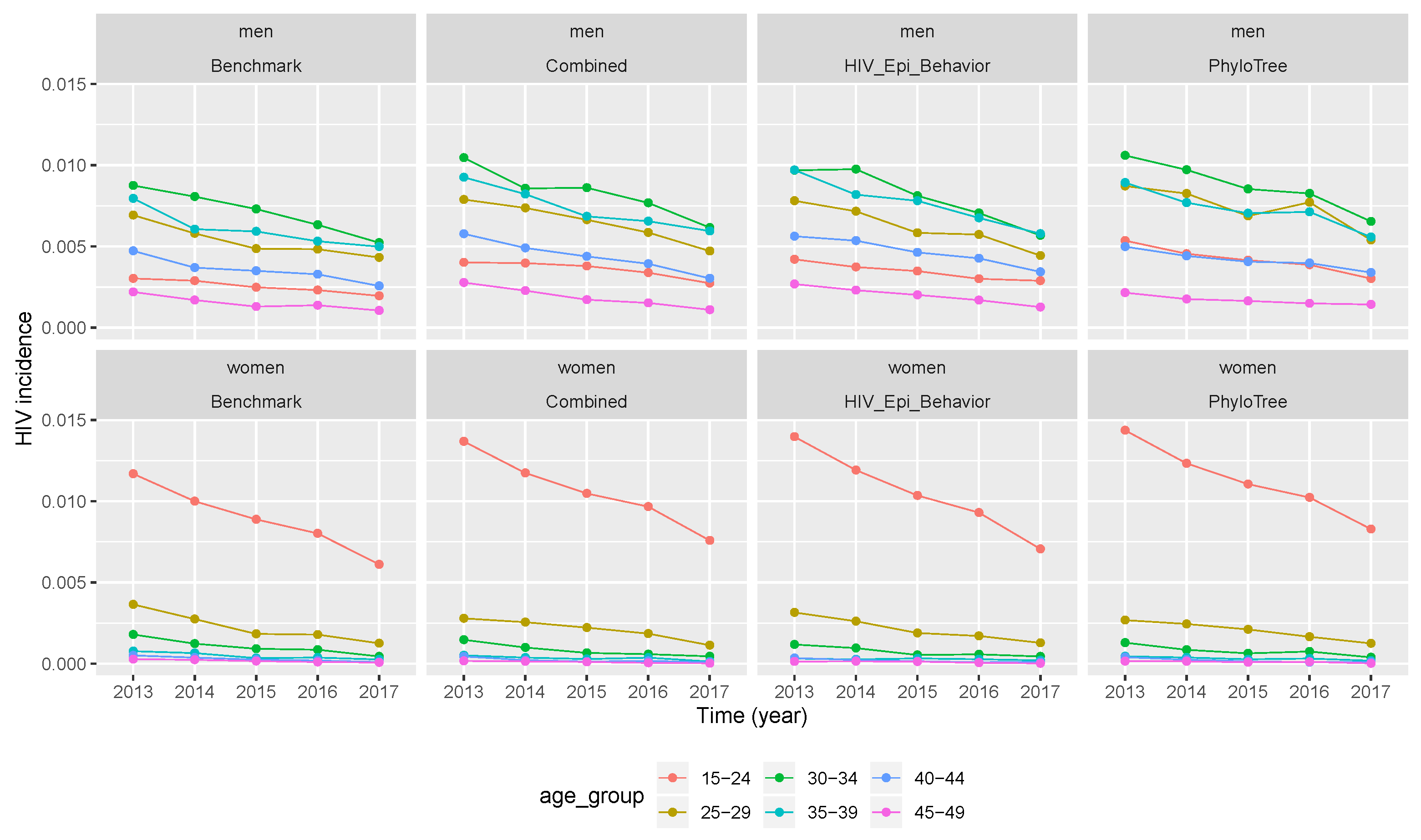
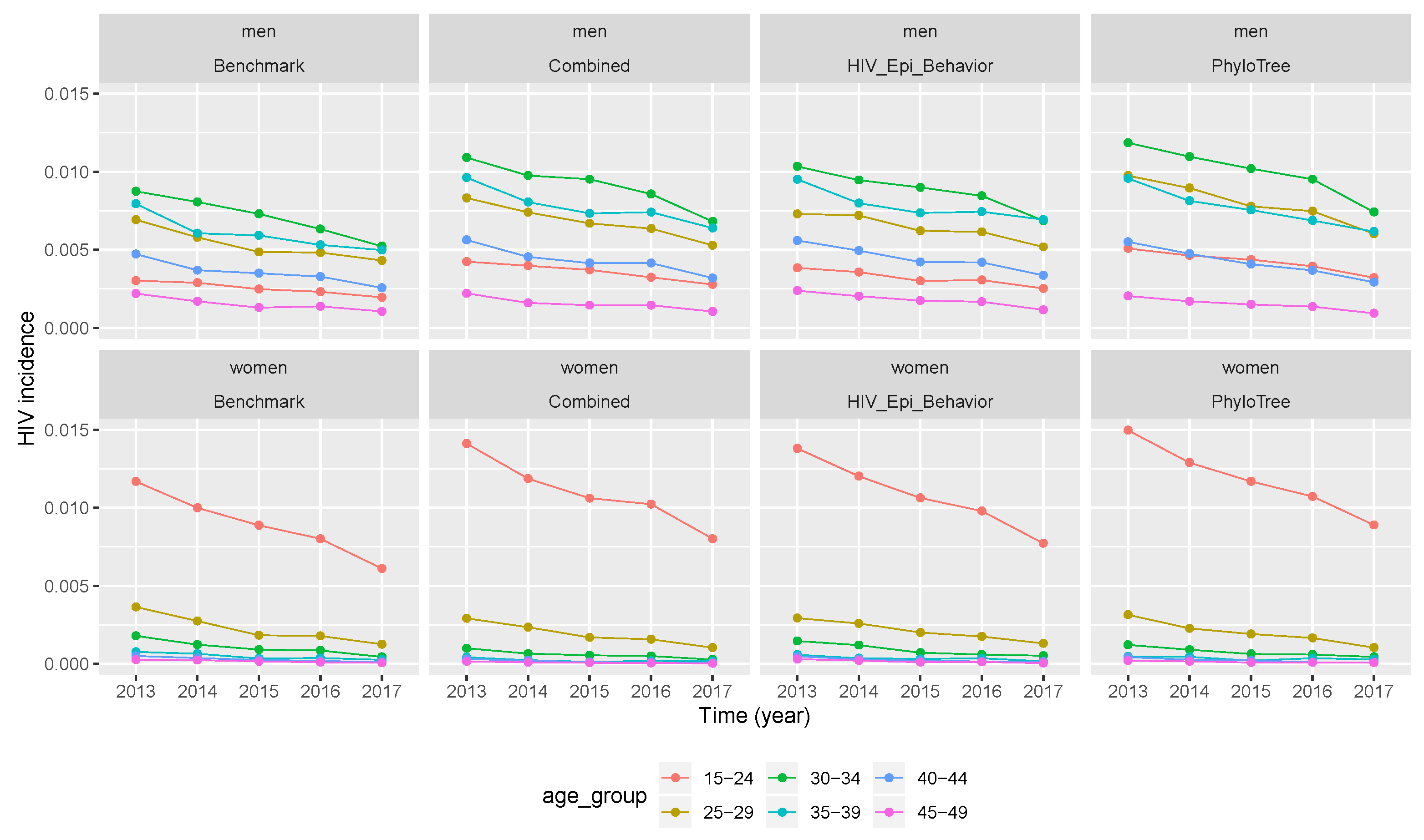
3.3. Temporal Trend of Hiv Incidence

The benchmark trend of incidence in the five year period (2012–2017) for men and women in different age groups (in the first column of Figure 4 or Figure 5) showed that it was decreasing in all gender and age groups. Younger women between 15 and 24 years had the highest incidence compared to other age groups in women and men. The decreasing trend meant that ART interventions had effects on HIV transmission.
After the three calibration scenarios, the incidence data points computed with vectors of retained parameters were presented in Figure 4. The comparison between the three scenarios and the benchmark (columns of Figure 4) showed that the temporal trend of incidence was over-estimated in almost all calibration scenarios. However, much more over-estimation was after calibration of the simulation framework with phylogenetic tree features, followed by the scenario of combined features. The same conclusion was drawn for Figure 5, where incidence values were computed after running the simulation framework with median values of retained parameter values after calibration.
As previously seen for other estimates, a two-by-two comparison of incidence obtained with vectors of the retained parameters (calibration columns without * in Table 5 and Table 6) and with median values of the retained parameters (calibration columns with * in Table 5 and Table 6) for each calibration scenario; we can see that the second option performed well although it does not give the best results of distribution of the temporal trend of HIV incidence.
If we consider mean relative error after calibration when the simulation was performed by median values of retained parameters (columns 4, 6, and 8) for both Table 5 and Table 6, the comparison between the error tables showed that men had higher error values compared to women. For the female population, younger women (15–24 years) had the lowest error values (Table 6).
When we compare the temporal trend of incidence between men and women (rows of Figure 4) for the benchmark and after calibration (in all three scenarios), we can see that incidence values for both populations had the same descending trend with time. The same conclusion was drawn from Figure 5, where incidence values were computed after running the simulation framework with median values of retained parameter values. However, when looking at the relative error, the latter did not decrease or increase with time. Thus, the over-estimation of incidence values did not vary with time, but across different age groups and gender as we can see in Table 5 and Table 6.

4. Conclusions

The objective of this simulation study was to investigate if accuracy of estimates obtained by calibration of the Simpact Cyan simulation framework with combined summary features can be improved. We expected that the estimates of HIV transmission network determinants (age-mixing patterns, distribution of onward HIV transmission, and temporal trend of HIV incidence) could be improved by fitting the simulation framework to combined summary features. From the values of mean relative errors in the three calibration scenarios, we have seen that we produced relatively the same outputs after calibration of the simulation framework by epidemiological and behavioural features, phylogenetic tree summary features, and combined features. Thus, any scenario can help to calibrate the simulation framework. These outputs results were supported by the parameter values retained in calibration for all scenarios (Table A4). When we look at these as shown in the Appendix B, we observe that all retained parameter values were closer to those used to generate benchmark data; the error between them was at the order of ten thousandths (Figure A1).
If we multiply error values by 100, for all calibration scenarios, AAD, SDAD, BSD, and WSD estimates of age-mixing patterns have less than 7% of mean relative error. However, the slope and intercept of the mixed effect model for age-mixing patterns had 8 and 16% of mean relative error, respectively. For the distribution of onward HIV transmission, the error for the mean was around 12%, whereas for the median and standard deviation it was around 30%. For the temporal incidence trend, the majority of incidence values had more than 100% of relative error, which made incidence the poorly depicted measurement after calibration.
Therefore, estimates of age-mixing patterns in sexual partnerships had relatively lower relative error (around 10%) when compared with the benchmark values and those obtained after calibration in any calibration scenario. They were followed by the distribution of onward HIV transmission.
Studies on sexual partnerships and age difference between partners showed that age gap in sexual partnerships and subsequent HIV transmission could be the main driver of the HIV transmission cycle between generations in some settings [18,47]. One of the studies used sero-conversion data from a population-based cohort of men and women [47], and another one used phylogenetic pairings from transmission clusters computed from a phylogenetic tree [18], both in KwaZulu Natal. Thus, as we have shown, Simpact Cyan can be calibrated with epi-behavioural and phylogenetic tree data, providing a technical platform to understand the effect of age-mixing patterns on HIV transmission dynamics, and their magnitude. The same advantage was observed for onward HIV transmissions. Thus, it is known that ART decreases HIV infections [48]; hence, we can investigate the effect of ART on incidence across different age groups between men and women.
The estimates of temporal incidence were not what we expected; the difference between benchmark values and estimates values are important. If Simpact Cyan can capture estimates of age-mixing patterns in sexual partnerships, and the distribution of onward HIV transmission, the reasons for poor estimates for temporal gender and age group strata of incidence trend could be a limitation due to the summary features we used. They could not depict incidence at different time points given the dynamic nature of sexual and transmission networks. We can see that, in the Appendix B, for summary features some were not converging, as we can see in Figure A2 and Figure A3. Such instability impedes the accuracy of post-calibration. Thus, when using Simpact Cyan for real-life estimation or prediction, given available summary features to be used, an exploratory study about the accuracy level of the outputs is advisable, and parameters which need to be turned.
Between the two options of post-calibration simulation: with vectors of retained parameter values, and with medians values of retained parameter values, we produced good estimates if we ran simulations several times (1120) with the median values of the retained parameter values. However, when we checked per each parameter, the number of retained parameter values was less than 1120, which we expected with 30% of the 3752 values; this was due to the fact that sometimes the simulation may produce NAs when the model executes events which are beyond the maximum cut-off number of events (see the configuration of population.maxevents in Simpact Cyan documentation [35]). This was conducted to discard unnecessary simulations with a lot of events in order to optimise memory use. Thus, the first option of the post-calibration simulation had less simulations run compared to the second option. The more we run the simulations, more we converge to the benchmark values.
Concerning the fact that the findings of temporal trends did not meet our expectations, we assume that perhaps the summary features we used were not good enough to depict age- and gender-stratified incidence. Therefore, an exploratory simulation study is required to determine the best summary features which would better suit estimation of temporal incidence trends. Such an exploratory study could help to provide a data-driven conclusion on this matter. However, since Simpact Cyan is a multipurpose tool which can simulate many epidemiological estimates at once, even before conducting exploratory studies on summary statistics, it is crucial to undertake a sensitivity analysis [49] for specific outputs of interest before calibration.
Simpact Cyan is an agent-based model tool, which makes it computationally intense and memory expensive [50]. With simulation of viral evolution, and computation of the phylogenetic tree, the memory and time demand increases. As such, the use of combined features come at a cost in terms of time and memory [30]. Thus, the results suggest that epidemiological and sexual behavioural features were enough to estimate HIV transmission network determinants.
Therefore, if we want to estimate or predict HIV-related measurements which do not necessarily need to use the phylogenetic tree, we can use other data sources which can be captured in Simpact Cyan to avoid computational constraints. However, when we do not have other data except phylogenetic tree data, we can use features from the phylogenetic tree to calibrate the simulation framework.
We have also seen that combined features give reliable results; thus, we can use epidemiological and behavioural, and phylogenetic tree features, in methodological research, if we want to investigate accuracy of phylogenetic tree-based inferences for HIV transmission networks. The combination of epidemiological and behavioural, and phylogenetic tree features, is a bridge between two components of the simulation framework model world, namely, HIV transmission network and viral evolution.
The results of this simulation study are a note of caution for calibration simulation studies to estimate some key parameters or key determinants related to the HIV epidemic using Simpact Cyan. This study has shown that all calibration scenarios are good in terms of accuracy of estimates in post calibration analysis. However, we have seen also that not every parameter can be estimated with high accuracy given different summary features. Thus, it is advisable to first generate benchmark data and check the level of accuracy for estimates of interest using the simulation framework given the available summary features from real world data. This will help to know to what extent the results can be trusted.

Author Contributions

Conceptualisation, D.N., T.C. and W.D.; methodology, D.N. and W.D.; software, D.N.; formal analysis, D.N. and T.C.; writing—original draft preparation, D.N., T.C. and P.S.N.; writing—review and editing, P.S.N., D.N., T.C. and W.D.; visualisation, D.N.; supervision, P.S.N. and W.D. of the project. All authors have read and agreed to the published version of the manuscript.

Funding

This research was funded by NRF-TWAS grant number 100014 for DN.

Institutional Review Board Statement

Not applicable, the study used model-based simulated data.

Informed Consent Statement

Not applicable, the study used model-based simulated data.

Data Availability Statement

The datasets generated and/or analysed during the current study are available in a Github repository (https://github.com/niyukuri/calibration_sympact, accessed on 15 November 2020).

Acknowledgments

The authors acknowledge the Centre for High Performance Computing (CHPC) at the University of Cape Town for providing computational resources for this project. DN would like to thank NRF-TWAS for the funding and SACEMA for hosting him during this project. We thank Emanuel Muema Dominic for his contribution during the study design.

Conflicts of Interest

The authors declare no conflict of interest. This work is based on the research supported by the Department of Science and Innovation (DSI) and the National Research Foundation (NRF). Any opinion, finding, and conclusion or recommendation expressed in this material is that of the authors and the DSI/NRF does not accept any liability in this regard. The funders had no role in the design of the study; in the analyses, or interpretation of data; in the writing of the manuscript, or in the decision to publish the results.

Appendix A. Simpact Cyan Simulation Model

Before running Simpact Cyan, it might be configured based on a simulation platform, and also the kind of sexual network to be simulated (heterosexual or same sex) across which HIV will be transmitted. To configure a simulation, you need to specify the options for which you want to use a value other than the default. Simpact Cyan has many parameters, as we can see in its documentation [35], and most of them were set given common knowledge, and findings from empirical studies. In this brief note, we provided description of parameters of interest which we tweaked for different events in the simulation model. More details are in the documentation of Simpact Cyan [35], where we extracted most of the content of this description note.
The simulation advances by figuring out which event should take place next, followed by the executing code for that event. At the start, many initial events are typically scheduled, some set up to fire at a specific simulation time, some based on a hazard which may change during the simulation. During the simulation, new events will be scheduled, and some already scheduled events will be discarded (for example, in case of someone dying, no other events involving this person will need to be executed). The occurrence rates of events is calculated by evaluating the hazard functions for those events. Many of the parameters come from hazard functions, but there are also other parameters related to settings of events, more details are provided in the hazard functions and parameters subsection.

Appendix A.1. Configuration

The configuration of Simpact Cyan is mainly based on creating an initial population, scheduling initial events, and setting parameter values for event occurrence hazard functions and related settings.

Appendix A.1.1. Create the Initial Population

Set a number of men (population.nummen) and women (population.numwomen) who make up the initial population. The population age is drawn from a defined Weibull survival distribution (shape = 5, scale = 65), in the absence of HIV-related mortality, for the population at the start of the simulation. Depending on the debut age (15 years), people may be marked as being ‘sexually active’.

Appendix A.1.2. Schedule the Initial Events

For each person, a ‘normal’ mortality event will be scheduled, and if needed, a debut event will be scheduled. Begin the HIV epidemic started at some point, by scheduling an HIV seeding event. If specified, schedule the next simulation intervention (ART). This is a general way of changing simulation settings during the simulation. For pairs of sexually active persons, depending on the ‘eyecap’ settings (population.eyecap.fraction), schedule formation events. This parameter allows specification of with how many persons of the opposite sex (who are sexually active), specified as a fraction, someone can possibly have relationships.
Once the simulation is started, it will run either until the number of years specified in population.simtime have passed, or until the number of events specified in population.maxevents have been executed.

Appendix A.1.3. Hazard Functions and Parameters

Simpact Cyan uses mathematical expressions which allow the values of events’ occurrence rates to depend on different factors which are known to influence the occurrence of events. For example, an event like relationship formation is affected by many factors such as age of the individual, ongoing sexual partnership, her/his age gap preference, among others; to capture their effect on the event’s occurrence and to ensure that the hazard of occurrence is bounded between zero 0 and plus infinite , the exponential function is a convenient candidate; hence, hazard functions are expressed as a linear expression raised to exponent.
h ( t ) = A × e x p B ( t )
Furthermore, for events which occur based on their hazard functions, we have specific settings related to events. For example, distribution of age preference between partners; this is a relationship-related setting among others, as we will see in subsequent sections.

Appendix A.2. Model Parameters: Events’ Hazard Functions and Associated Settings

The parameters, we chose, which are in Table A4, were from the following hazard functions, and event-related settings:

Appendix A.2.1. Sexual Partnership Event

hazard rel = F × exp α baseline + α numrel , man P man ( 1 + α numrel , scale , man g man ( t ry ) ) + α numrel , woman P woman ( 1 + α numrel , scale , woman g woman ( t ry ) ) + α numrel , diff | P man P woman | + α meanage A man ( t ) + A woman ( t ) 2 + α dist | R man R woman | + α eagerness , sum ( E man + E woman ) + α eagerness , diff | E man E woman | + G man ( t ry ) + G woman ( t ry ) + β ( t t ref )
where
G man ( t ry ) = [ α gap , factor , man , const + α gap , factor , man , exp exp α gap , factor , man , age A man ( t ry ) A debut ] × | g man ( t ry ) |
and
G woman ( t ry ) = [ α gap , factor , woman , const + α gap , factor , woman , exp exp α gap , factor , woman , age A woman ( t ry ) A debut ] × | g woman ( t ry ) |
For the sexual partnership event, the parameters we tweaked in the simulation were:
  • f o r m a t i o n . h a z a r d . a g e g a p r y . b a s e l i n e , the value of α baseline in the expression for the hazard, allowing one to establish a baseline value.
  • f o r m a t i o n . h a z a r d . a g e g a p r y . g a p . a g e s c a l e . m a n controls α gap , agescale , man , which allows you to vary the preferred age gap with the age of the man in the relationship; and
  • f o r m a t i o n . h a z a r d . a g e g a p r y . g a p . a g e s c a l e . w o m a n controls α gap , agescale , woman , which allows you to vary the preferred age gap with the age of the woman in the relationship.
  • f o r m a t i o n . h a z a r d . a g e g a p r y . n u m r e l . m a n , the value of α numrel , man in the hazard formula, corresponding to a weight for the number of relationships the man in the relationship has; and
  • f o r m a t i o n . h a z a r d . a g e g a p r y . n u m r e l . w o m a n , the value of α numrel , woman in the hazard formula, corresponding to a weight for the number of relationships the woman in the relationship has.
  • f o r m a t i o n . h a z a r d . a g e g a p r y . n u m r e l . d i f f , the value of α numrel , diff in the hazard expression, by which the influence of the difference in number of partners can be specified.
  • f o r m a t i o n . h a z a r d . a g e g a p r y . m e a n a g e , the value of weight of α m e a n a g e in the expression for the hazard, a weight for the average age of the partners.

Appendix A.2.2. Sexual Partnership Dissolution Event

hazard diss = exp α 0 + α 1 P man + α 2 P woman + α 3 | P woman P man | + α 4 ( t t birth , man ) + ( t t birth , woman ) 2 + α 5 | ( t t birth , man ) ( t t birth , woman ) D pref | + β ( t t ref )
For a sexual partnership dissolution event, the parameters we tweaked in the simulation were:
  • d i s s o l u t i o n . a l p h a . 0 , the value of α 0 in the expression for the hazard, allowing one to establish a baseline value.
  • d i s s o l u t i o n . a l p h a . 1 , the value of α 1 in the expression for the hazard, corresponding to a weight for the number of relationships the man in the relationship has.

Appendix A.2.3. Relationship-Related Settings

Moreover, defined factors mentioned in Appendix A.2.1 which influence sexual partnerships might depend also on individual eagerness, and age gap preference. Relationship settings define known facts that influence sexual partnerships, and which are set by probability distributions in Simpact Cyan.

Eagerness

The eagerness of a person to form a relationship is used to allow a person’s variation to engage in sexual partnership. Such an eagerness value can be defined for heterosexual relationships ( p e r s o n . e a g e r n e s s . m a n . d i s t . t y p e and p e r s o n . e a g e r n e s s . w o m a n . d i s t . t y p e ) and same sex relationships ( p e r s o n . e a g e r n e s s . m a n . m s m . d i s t . t y p e and p e r s o n . e a g e r n e s s . w o m a n . w s w . d i s t . t y p e ) independently, or a correlation can be introduced by using a joint distribution ( p e r s o n . e a g e r n e s s . m a n . j o i n t . d i s t 2 d and p e r s o n . e a g e r n e s s . w o m a n . j o i n t . d i s t 2 d ). In the latter case, a pair of numbers is generated from a distribution, of which the first number is interpreted as the eagerness for a heterosexual relationship and the second for a same sex relationship. By default, independent random numbers are used, but this can be changed using the configuration value of p e r s o n . e a g e r n e s s . m a n . t y p e and p e r s o n . e a g e r n e s s . w o m a n . t y p e .
In our simulation the distribution type was a gamma distribution; thus, we tweaked the following parameters related to eagerness:
  • p e r s o n . e a g e r n e s s . m a n . d i s t . g a m m a . a , represents α parameter for a man’s eagerness following a gamma distribution
  • p e r s o n . e a g e r n e s s . w o m a n . d i s t . g a m m a . a , represents α parameter for a woman’s eagerness following a gamma distribution
  • p e r s o n . e a g e r n e s s . m a n . d i s t . g a m m a . b , represents β parameter for a man’s eagerness following a gamma distribution
  • p e r s o n . e a g e r n e s s . w o m a n . d i s t . g a m m a . b , represents β parameter for a woman’s eagerness following a gamma distribution

Age Gap Preference

Similarly to eagerness, preferred age gaps can be used in hazards, and these also can be defined for each person separately. Moreover, they can differ between heterosexual relationships: p e r s o n . a g e g a p . m a n . d i s t . t y p e and p e r s o n . a g e g a p . w o m a n . d i s t . t y p e , and same sex: p e r s o n . a g e g a p . m a n . m s m . d i s t and p e r s o n . a g e g a p . w o m a n . w s w . d i s t .
In our simulation, the distribution type was a normal distribution; thus, we tweaked the following parameters related to age gap preference:
  • p e r s o n . a g e g a p . m a n . d i s t . n o r m a l . m u , for a man’s mean of normal distribution of age preference between men and women
  • p e r s o n . a g e g a p . w o m a n . d i s t . n o r m a l . m u , for a woman’s mean of normal distribution of age preference between women and men
  • p e r s o n . a g e g a p . m a n . d i s t . n o r m a l . s i g m a , for a man’s standard deviation of normal distribution of age preference between men and women
  • p e r s o n . a g e g a p . w o m a n . d i s t . n o r m a l . s i g m a , for a woman’s standard deviation of normal distribution of age preference between women and men

HIV Transmission Event

When a relationship is formed between two people of which one is HIV infected, or when a relationship between two uninfected people exists and one of them is infected, an HIV transmission event is scheduled. The hazard for this event is the following:
hazard trans = exp a + b V c + d 1 P infected + d 2 P uninfected + W f 1 exp ( f 2 ( A woman ( t ry ) A debut ) ) + e 1 H S V 2 infected + e 2 H S V 2 uninfected + g 1 b 0 j + g 2 b 1 j
For an HIV transmission event, the hazard function can also be estimated in terms of a transmission probability [51], the parameters we tweaked in the simulation were:
  • h i v t r a n s m i s s i o n . p a r a m . a refers to the value of a in the expression for the hazard, providing a baseline value.
  • h i v t r a n s m i s s i o n . p a r a m . b refers to the value of b in the expression for the hazard. Together with the value of c this specifies the influence of the current viral load of the infected person.
  • h i v t r a n s m i s s i o n . p a r a m . c refers to the value of c in the expression for the hazard. Together with the value of b, this specifies the influence of the current viral load of the infected person.
  • h i v t r a n s m i s s i o n . p a r a m . f 1 refers to the value of f 1 in the expression of the hazard.
  • h i v t r a n s m i s s i o n . p a r a m . f 2 refers to the value of f 2 in the expression of the hazard. Furthermore, by configuring the weights f 1 and f 2 , it becomes possible to change the susceptibility of a woman depending on her age.

Appendix A.2.4. Hiv Infection Monitoring Event

When a person has been diagnosed as being infected with HIV, monitoring events are scheduled to follow up on the progress of the disease by inspecting the person’s Cluster of Differentiation 4 (CD4) count. If this CD4 count is below the threshold set in m o n i t o r i n g . c d 4 . t h r e s h o l d , the person will be offered antiretroviral treatment. Depending on the person’s willingness to accept treatment, treatment will then be started.
For an HIV infection monitoring event, the parameters we tweaked in the simulation were:
  • m o n i t o r i n g . c d 4 . t h r e s h o l d parameter for the threshold set for the infected person to be offered antiretroviral treatment.
  • m o n i t o r i n g . f r a c t i o n . l o g . v i r a l l o a d parameter to lower the person’s set-point viral load value if treatment is started.
  • p e r s o n . a r t . a c c e p t . t h r e s h o l d . d i s t . f i x e d . v a l u e ART acceptance.

Appendix A.2.5. Diagnosis Event

When a person is infected with HIV, either by transmission of the virus or by seeding the population to start the epidemic, a diagnosis event will be scheduled. When fired, the person is deemed to feel bad enough to go to a doctor and is diagnosed as being HIV-infected. Upon diagnosis, a monitoring event will be scheduled very shortly afterwards, to monitor the progression of the disease and to offer treatment if eligible. This event is hazard-based, and the hazard is of the following form:
hazard diag = exp ( baseline + agefactor × ( t t birth ) + genderfactor × G + diagpartnersfactor × P + isdiagnosedfactor × D + β ( t t infected ) + HSV 2 factor × HSV 2 )
For a diagnosis event, the only parameter we tweaked in the simulation was:
  • d i a g n o s i s . b a s e l i n e controls the corresponding baseline value in the expression for the hazard.
Other parameters were set to zero in our simulation, and details about them can be found in the documentation.

Appendix A.2.6. Hiv Infection Stage and Viral Load

When a person becomes HIV-infected, either by an HIV seeding event or because of transmission of the virus, a set-point viral load value is chosen and stored for this person. When a person receives treatment, the viral load is lowered (see the monitoring event) and, if the person drops out of treatment the initially chosen set-point, the viral load is restored. The set-point viral load is the viral load that the person has during the chronic stage.
For further stages we have the following parameters, which were tweaked in our simulation:
  • p e r s o n . v s p . t o a c u t e . x : when the viral load during the acute stage is needed, it is determined in such a way that the transmission hazard increases by this factor, possibly clipped to a maximum value ( p e r s o n . v s p . m a x v a l u e ).
  • p e r s o n . v s p . t o a i d s . x : when the viral load during the initial AIDS stage is needed, it is determined in such a way that the transmission hazard increases by this factor, possibly clipped to a maximum value ( p e r s o n . v s p . m a x v a l u e ).
  • p e r s o n . v s p . t o f i n a l a i d s . x : when the viral load during the final AIDS stage is needed, it is determined in such a way that the transmission hazard increases by this factor, possibly clipped to a maximum value ( p e r s o n . v s p . m a x v a l u e ).
In any of the stages, when determining the viral load during acute, AIDS or final AIDS stages, a check is performed so that the value does not exceed this maximum. If necessary, the calculated viral load value is clipped to this maximum value.

Appendix A.2.7. Art Treatment Dropout Event

When a monitoring event is triggered and the person is both eligible and willing to receive treatment, treatment is started, causing the set-point viral load of the person to be lowered. When treatment starts, a dropout event is scheduled as well, to allow a person to drop out of treatment.
Currently, the dropout event is not hazard-based, instead a random number is picked from a one dimensional probability distribution as specified in d r o p o u t . i n t e r v a l . d i s t . t y p e and related configuration options.
Using this configuration option you can specify the probability distribution to use when obtaining the time after which a person will drop out of treatment. By default, this is a uniform distribution with equal non-zero probability between 3 months and 10 years, and zero otherwise. Other distributions can be specified as well, as explained previously.

Appendix A.2.8. Aids Mortality Event

When a person is infected with HIV, an HIV-based time of death is determined. This time of death is determined as the time of infection plus the survival time as explained in the following formula [52]:
t survival = C V s p k × 10 x
where V s p is the set-point viral load, x a parameter determined per person to allow randomness.
For an AIDS mortality event, the parameters we tweaked in the simulation were:
  • C is set in the model by m o r t a l i t y . a i d s . s u r v t i m e . C
  • k is set in the model by m o r t a l i t y . a i d s . s u r v t i m e . k
By default, the survival time for a person after becoming HIV infected is given by a simple relation based on the set-point viral load. Because an exact mapping from viral load to survival time is not that realistic, you can add some randomness to this relation using the distribution in p e r s o n . s u r v t i m e . l o g o f f s e t . d i s t . t y p e . When a person becomes infected, a random number is drawn from this distribution and will correspond to an offset in the survival time, as explained in the AIDS mortality event.
  • p e r s o n . s u r v t i m e . l o g o f f s e t . d i s t . t y p e one dimensional distribution can be used to add some randomness to the survival time until the person dies of AIDS-related causes after becoming infected with HIV.

Appendix A.2.9. Conception Event

When a formation event has fired (so a man and a woman are in a sexual relationship), a conception event will be scheduled unless the woman is already pregnant. This is a hazard-based event, and its hazard at time t is defined as:
hazard conc = exp ( α base + α age , man t t birth , man + α age , woman t t birth , woman + α wsf × WSF + ( t t ref ) β )
For a conception event, the only parameter we tweaked in the simulation was:
  • α base set by c o n c e p t i o n . a l p h a . b a s e baseline for a conception hazard function
By default, only the α base value is used ( c o n c e p t i o n . a l p h a b a s e ), resulting in a constant hazard, but other factors can be used as well: the age of the man and woman in the relationship can be taken into account using c o n c e p t i o n . a l p h a . a g e m a n and c o n c e p t i o n . a l p h a . a g e w o m a n , the weekly sex frequency (WSF) using c o n c e p t i o n . a l p h a . w s f and the ‘age’ of the relationship using conception.beta (tref is set to the time the relationship started). The value of WSF itself is currently chosen from the distribution specified in c o n c e p t i o n . w s f . d i s t . t y p e , at the time the event is scheduled.
Table A1. Values of selected parameters for the simulation of HIV epidemic.
ParameterExplanationValue
Initial configuration
p o p u l a t i o n . s i m t i m e Simulation time40
p o p u l a t i o n . m s m Same sex sexual partnershipno
p o p u l a t i o n . n u m m e n Initial male population5000
p o p u l a t i o n . n u m w o m e n Initial female population5000
h i v s e e d . t i m e Time to introduce HIV into the population10
h i v s e e d . t y p e Consider the amount not proportion of seeded individuals among the population
h i v s e e d . a m o u n t Amount of HIV seeded individuals10
h i v s e e d . a g e . m i n Minimum age for seeded individuals20
h i v s e e d . a g e . m a x Maximum age for seeded individuals50
d e b u t . d e b u t a g e Age of being sexually active15
p o p u l a t i o n . m a x e v e n t s Maximum events to be simulated (beyond this number of events, the simulation will stop, it can also stop with population.simtime)1.2 million 1
p o p u l a t i o n . e y e c a p . f r a c t i o n Specify how many persons of the opposite sex (who are sexually active), specified as a fraction, someone can possibly have relationships0.2
Demographic
b i r t h . b o y g i r l r a t i o boy/girl ratio 1.0 / 2.01
c o n c e p t i o n . a l p h a . b a s e Baseline for conception event 3
Sexual partnership
p e r s o n . e a g e r n e s s . m a n . d i s t . g a m m a . a α parameter for male eagerness following a gamma distribution0.23
p e r s o n . e a g e r n e s s . w o m a n . d i s t . g a m m a . a α parameter for female eagerness following a gamma distribution0.23
p e r s o n . e a g e r n e s s . m a n . d i s t . g a m m a . b b e t a parameter for male eagerness following a gamma distribution45
p e r s o n . e a g e r n e s s . w o m a n . d i s t . g a m m a . b b e t a parameter for female eagerness following a gamma distribution45
p e r s o n . a g e g a p . m a n . d i s t . t y p e Distribution type for age gap preference for menNormal
p e r s o n . a g e g a p . w o m a n . d i s t . t y p e Distribution type for age gap preference for womenNormal
f o r m a t i o n . h a z a r d . a g e g a p r y . b a s e l i n e Baseline for sexual partnerships2
p e r s o n . a g e g a p . m a n . d i s t . n o r m a l . m u Mean for the normal distribution of the age gap preference for men10
p e r s o n . a g e g a p . w o m a n . d i s t . n o r m a l . m u Mean for the normal distribution of the age gap preference for women10
p e r s o n . a g e g a p . m a n . d i s t . n o r m a l . s i g m a Standard deviation for the normal distribution of the age gap preference for men5
p e r s o n . a g e g a p . w o m a n . d i s t . n o r m a l . s i g m a Standard deviation for the normal distribution of the age gap preference for women5
f o r m a t i o n . h a z a r d . a g e g a p r y . g a p . a g e s c a l e . m a n Allows varying of the preferred age gap with the age of the man in the relationship 0.25
f o r m a t i o n . h a z a r d . a g e g a p r y . g a p . a g e s c a l e . w o m a n Allows varying of the preferred age gap with the age of the woman in the relationship 0.25
f o r m a t i o n . h a z a r d . a g e g a p r y . n u m r e l . m a n Corresponding to a weight for the number of relationships the man in the relationship has−0.3
f o r m a t i o n . h a z a r d . a g e g a p r y . n u m r e l . w o m a n Corresponding to a weight for the number of relationships the man in the relationship has−0.3
f o r m a t i o n . h a z a r d . a g e g a p r y . n u m r e l . d i f f Influence of the difference in number of partners can be specified−0.1
d i s s o l u t i o n . a l p h a 0 Baseline for relationship dissolution 0.52
d i s s o l u t i o n . a l p h a 4 Weight for the average age of the partners in relationship dissolution 0.05
HIV transmission
h i v t r a n s m i s s i o n . p a r a m . a Baseline value for HIV transmission. 1
h i v t r a n s m i s s i o n . p a r a m . b Influence of the current viral load of the infected person. 90
h i v t r a n s m i s s i o n . p a r a m . c Influence of the current viral load of the infected person. 0.5
h i v t r a n s m i s s i o n . p a r a m . f 1 Weight for susceptibility of a woman depending on her age. 0.048
h i v t r a n s m i s s i o n . p a r a m . f 2 Weight for susceptibility of a woman depending on her age. 0.14
HIV infection stages
p e r s o n . v s p . t o a c u t e . x Viral load during the acute stage.5
p e r s o n . v s p . t o a i d s . x Viral load during the initial AIDS stage.7
p e r s o n . v s p . t o f i n a l a i d s . x Viral load during the final AIDS stage.12
HIV infection monitoring
m o n i t o r i n g . f r a c t i o n . l o g v i r a l l o a d Lower the person’s set-point viral load value when someone started ART.0
ART interventions
For ART intervention we have:
t i m e Time for ART intervention
d i a g n o s i s . b a s e l i n e Diagnosis baseline
m o n i t o r i n g . c d 4 . t h r e s h o l d CD4 count eligibility cutoff
ART introduction 1:
t i m e 23 (2000 **)
d i a g n o s i s . b a s e l i n e −2
m o n i t o r i n g . c d 4 . t h r e s h o l d 100
ART introduction 2:
t i m e 25 (2002 **)
d i a g n o s i s . b a s e l i n e −1.8
m o n i t o r i n g . c d 4 . t h r e s h o l d 150
ART introduction 3:
t i m e 28 (2005 **)
d i a g n o s i s . b a s e l i n e −1.5
m o n i t o r i n g . c d 4 . t h r e s h o l d 200
ART introduction 4:
t i m e 33 (2010 **)
d i a g n o s i s . b a s e l i n e −1
m o n i t o r i n g . c d 4 . t h r e s h o l d 350
ART introduction 5:
t i m e 36 (2013 **)
d i a g n o s i s . b a s e l i n e −1
m o n i t o r i n g . c d 4 . t h r e s h o l d 500
ART introduction 6:
t i m e 39 (2016 **)
d i a g n o s i s . b a s e l i n e −1
m o n i t o r i n g . c d 4 . t h r e s h o l d 700
p e r s o n . a r t . a c c e p t . t h r e s h o l d . d i s t . f i x e d . v a l u e ART acceptance 0.75
d r o p o u t . i n t e r v a l . d i s t . t y p e Specification of ART dropout distributionUniform
d r o p o u t . i n t e r v a l . d i s t . u n i f o r m . m i n Minimum value of the uniform dropout distribution
d r o p o u t . i n t e r v a l . d i s t . u n i f o r m . m a x Maximum value of the uniform dropout distribution
AIDS mortality and survival
m o r t a l i t y . a i d s . s u r v t i m e . C Relationship between set-point viral load and survival.65
m o r t a l i t y . a i d s . s u r v t i m e . k Relationship between set-point viral load and survival.−0.2
p e r s o n . s u r v t i m e . l o g o f f s e t . d i s t . t y p e Type of distribution type for survival time randomness.Normal
p e r s o n . s u r v t i m e . l o g o f f s e t . d i s t . n o r m a l . m u Mean of the normal distribution for survival time randomness.
p e r s o n . s u r v t i m e . l o g o f f s e t . d i s t . n o r m a l . s i g m a Standard deviation of the normal distribution for survival time randomness.
1 We set the maximum events to 3× simulation time × initial male population; ** simulation time in calendar time (years).
Table A2. Main assumptions for the simulation of the dynamic sexual partnership network and HIV transmission.
Sub-ComponentAssumptions
DemographicBirth: when there is a sexual partnership formation, a conception event will be scheduled; after a conception event is triggered, a new birth event will be scheduled, so that the woman in the relationship will give birth to a new person at a specific time, and the gender will be determined by the boy/girl ratio. Mortality: normal mortality model follows Weibull distribution, and the time for AIDS mortality was determined as the time of infection plus the survival time.
Sexual partnershipWe considered sexual partnerships such that the preferred age gap differed from one person to the next, but there was also an age dependent component in this preferred age gap, and we allowed for the weight of the age gap terms to be age-dependent. We assumed the age gap to be normally distributed. The hazard function for partnership depended on the number of partners the man and woman in the relationship had. The debut age was set to be 15 years for men and women. Once a sexual partnership was established, it was subject to dissolution as well.
HIV transmissionTransmission is likely to occur when one individual in a sexual partnership is infected with HIV. Transmission depends on the viral load level of an infected individual. A woman’s susceptibility to HIV infection was considered to depend on her age. Set-point viral load is the viral load that the person has during the chronic stage. In the acute stage or in the Acquired immunodeficiency syndrome (AIDS) stages, the configuration values p e r s o n . v s p . t o a c u t e . x , p e r s o n . v s p . t o a i d s . x and p e r s o n . v s p . t o f i n a l a i d s . x cause the real viral load to differ from the set-point viral load in such a way that the transmission probability is altered: the hazard for transmission will increase by the factor x that is defined in this way. We also assumed that, once an infected individual is on ART, s/he cannot transmit the infection; thus, we set m o n i t o r i n g . f r a c t i o n . l o g v i r a l l o a d to 0.
ART interventionsIf this CD4 count is below the threshold set in m o n i t o r i n g . c d 4 . t h r e s h o l d , the person will be offered antiretroviral treatment (ART). Depending on the person’s willingness to accept treatment, treatment will then be started. We considered gradually increasing ART eligibility based on CD4 count thresholds as implemented in real life.
Disease progressionFollow up on the progress of the disease is performed by inspecting the person’s CD4 count. When a person receives treatment, the viral load is lowered and if the person drops out of treatment the viral load will increase.

Appendix A.3. Hiv Evolutionary Dynamic

For the HIV evolutionary dynamic, we considered population-level variation of viral sequence of substitutions of the nucleotide. To simulate viral sequence data for infected individuals, we used a full transmission tree of infected individuals and root sequence data. Each seeded individual who introduced HIV has his/her own transmission network, which was transformed into a transmission tree using the e p i 2 t r e e function of the R package e x p o T r e e [53]. We recursively combined all the transmission trees of the seed individuals (10), and built one transmission tree. We transformed the new tree into a binary tree using the m u l t i 2 d i function of the R package p h y t o o l s [54]. The final tree was used for a forward simulation of substitutions of the viral sequences (each per individual) using the G T R + Γ substitution model in Seq-Gen [41]. The root sequence was an HIV-1 sub-type C [55], and for simplicity we considered only the polymerase (POL) gene [56]. Model parameters in Table A3, were estimated using jModelTest 2.1.3 [57], on a large dataset of HIV-1 subtype C sequences from LOS ALAMOS.
Table A3. Parameters for the HIV 1 substitution G T R + Γ + I model.
NameValue
Relative Frequencies
Adenine (A)0.3857
Cytosine (C)0.1609
Guanine (G)0.2234
Thymine (T)0.2300
Relative substitution rates
r(A → G) = r(G → A)2.9114
r(A → C) = r(C → A)12.5112
r(A → T) = r(T → A)1.2569
r(G → C) = r(C → G)0.8559
r(G → T) = r(T → G)12.9379
r(C → T) = r(T → C)1.0000
Rate heterogeneity
Shape parameter0.9
Number of gamma rate categories4
Fraction of invariant sites
Proportion of invariant sites (I)0.5230
Evolutionary rate
Substitutions/site/year 2 4.75 × 10 3
2 which is the branch length scaling factor.
We acknowledged that, although consensus sequences of HIV remain useful for phylogenetic analysis at population level studies, there is high variability of the virus at within-host level in contrast with the low variability at the population level [58]. In addition, many questions of evolutionary dynamics still remain unexplained to date [59,60,61]; hence, it is still challenging to understand HIV phylodynamics clearly across scales [61,62,63]. However, the simplifications we made by only considering between-host variability are in line with population-level transmission network analysis using standard phylogenetic methods [20].

Appendix B. Calibration of Simpact Cyan: Parameters and Summary Features

To generate the benchmark data, we used the parameter values given in Table A1 and Table A3. To calibrate the tool we only considered the 13 parameter values of the input vector.

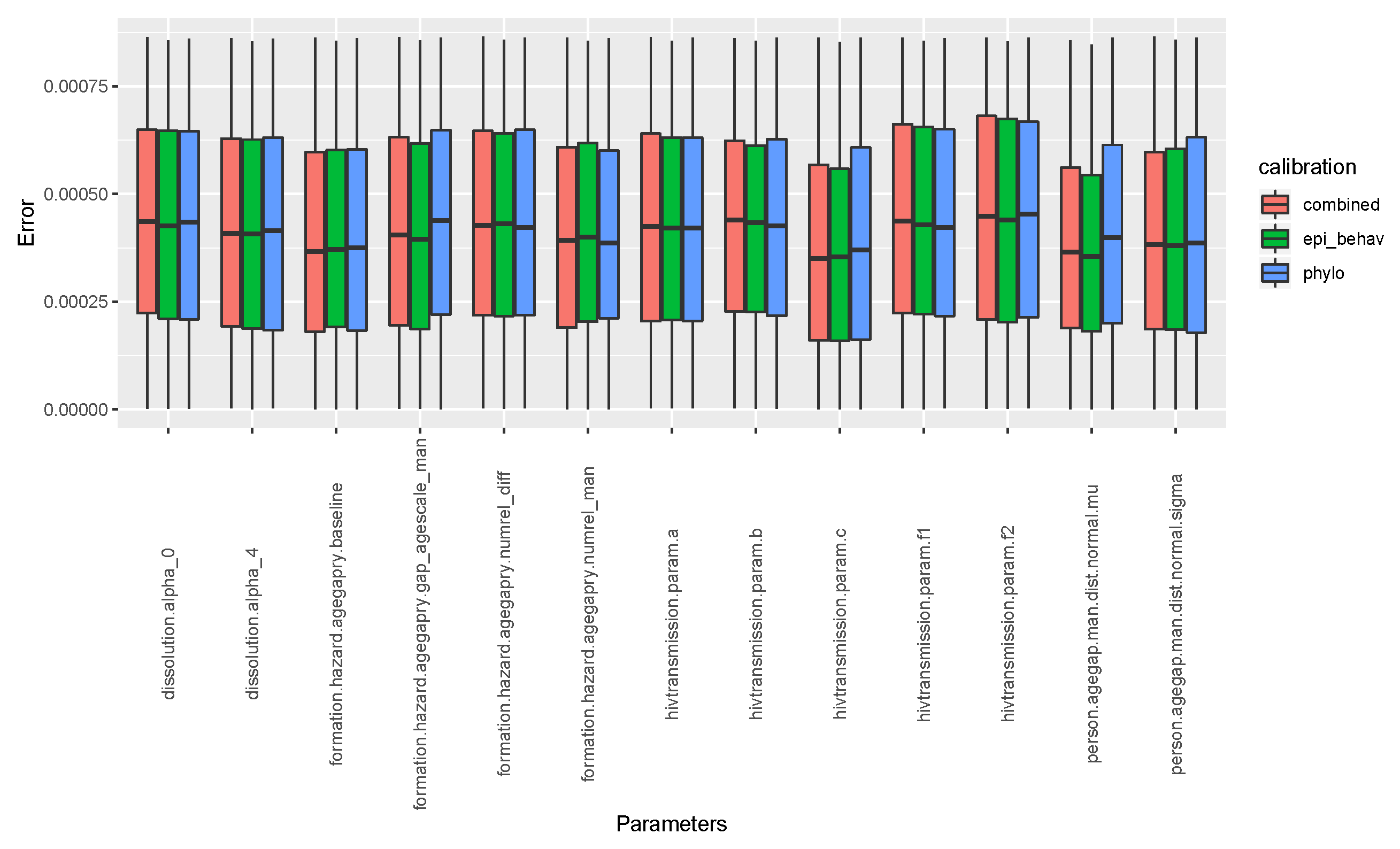
Appendix B.1. Selected Parameters for Calibration

As we said, Simpact Cyan has many parameters; the parameters we considered in our calibration exercise were coming from relationship establishment/dissolution, and HIV transmission hazard functions and related settings, which are described in the Appendix A. The piece of code of these parameters is given below. The benchmark values of these selected parameters (“Input” column of Table A4), and the values we obtained during calibration, are given in Table A4 (calibration columns).
cfg.list["dissolution.alpha_0"] <- inputvector[1]
cfg.list["dissolution.alpha_4"] <- inputvector [2]
cfg.list["formation.hazard.agegapry.baseline"] <- inputvector[3]
cfg.list["person.agegap.man.dist.normal.mu"] <- inputvector[4]
cfg.list["person.agegap.woman.dist.normal.mu"] <- inputvector[4]
cfg.list["person.agegap.man.dist.normal.sigma"] <- inputvector[5]
cfg.list["person.agegap.woman.dist.normal.sigma"] <- inputvector[5]
cfg.list["formation.hazard.agegapry.gap_agescale_man"] <- inputvector[6]
cfg.list["formation.hazard.agegapry.gap_agescale_woman"] <- inputvector[6]
cfg.list["formation.hazard.agegapry.numrel_man"] <- inputvector[7]
cfg.list["formation.hazard.agegapry.numrel_woman"] <- inputvector[7]
cfg.list["formation.hazard.agegapry.numrel_diff"] <- inputvector[8]
cfg.list["hivtransmission.param.a"] <- inputvector[9]
cfg.list["hivtransmission.param.b"] <- inputvector[10]
cfg.list["hivtransmission.param.c"] <- inputvector[11]
cfg.list["hivtransmission.param.f1"] <- inputvector[12]
cfg.list["hivtransmission.param.f2"] <- inputvector[13]
		    
We considered 13 parameter values, but some parameters such as person.agegap.man.dist.  n o r m a l . m u and p e r s o n . a g e g a p . w o m a n . d i s t . n o r m a l . m u (inputvector[4]) had the same values. This is the same for inputvector[5], inputvector[6], and inputvector[7].
Table A4. Median values and inter-quantile range for retained parameter values during calibration with epidemiological and behavioural features (Calibration 1), phylogenetic tree features (Calibration 2), and combined features (Calibration 3); together with input values used to run the master model (benchmark data), and the search parameter space for calibration.
Parameter Calibration 1 Calibration 2 Calibration 3 Input Space
d i s s o l u t i o n . a l p h a . 0 −0.514 [−0.654, −0.397] −0.52 [−0.652, −0.39] −0.514 [−0.653, −0.391] −0.52 [−0.78, −0.26]
d i s s o l u t i o n . a l p h a . 4 −0.053 [−0.064, −0.041] −0.052 [−0.063, −0.04] −0.053 [−0.064, −0.041] −0.05 [−0.075, −0.025]
f o r m a t i o n . h a z a r d . a g e g a p r y . b a s e l i n e 1.957 [1.513, 2.401] 1.976 [1.546, 2.409] 1.965 [1.54, 2.398] 2 [1, 3]
p e r s o n . a g e g a p . m a n . d i s t . n o r m a l . m u 10.277 [8.287, 12.324] 9.666 [7.433, 11.913] 10.11 [7.949, 12.195] 10 [5, 15]
f o r m a t i o n . h a z a r d . a g e g a p r y . g a p . a g e s c a l e . m a n 4.898 [3.84, 6.128] 4.989 [3.728, 6.248] 4.96 [3.839, 6.191] 5 [2.5, 7.5]
p e r s o n . a g e g a p . m a n . d i s t . n o r m a l . s i g m a 0.255 [0.2, 0.308] 0.244 [0.186, 0.299] 0.252 [0.198, 0.306] 0.25 [0.125, 0.375]
f o r m a t i o n . h a z a r d . a g e g a p r y . n u m r e l . m a n −0.299 [−0.371, −0.23] −0.302 [−0.37, −0.237] −0.302 [−0.371, −0.239] −0.3 [−0.45, −0.15]
f o r m a t i o n . h a z a r d . a g e g a p r y . n u m r e l . d i f f −0.101 [−0.126, −0.076] −0.099 [−0.122, −0.074] −0.1 [−0.124, −0.075] −0.1 [−0.15, −0.05]
h i v t r a n s m i s s i o n . p a r a m . a −1.016 [−1.215, −0.739] −0.977 [−1.195, −0.726] −0.997 [−1.216, −0.739] −1 [−1.5, −0.5]
h i v t r a n s m i s s i o n . p a r a m . b −85.888 [−109.426, −65.1] −84.888 [−107.133, −64.703] −85.927 [−109.915, −65.038] −90 [−135, −45]
h i v t r a n s m i s s i o n . p a r a m . c 0.589 [0.501, 0.662] 0.599 [0.512, 0.676] 0.59 [0.507, 0.662] 0.5 [0.25, 0.75]
h i v t r a n s m i s s i o n . p a r a m . f 1 0.048 [0.036, 0.061] 0.048 [0.036, 0.06] 0.048 [0.036, 0.06] 0.048 [0.024, 0.072]
h i v t r a n s m i s s i o n . p a r a m . f 2 −0.142 [−0.177, −0.106] −0.142 [−0.18, −0.106] −0.141 [−0.177, −0.105] −0.14 [−0.21, −0.07]

Appendix B.2. Parameter Space

The calibration of the default modelling framework is conducted to obtain best guesses of the best fit parameter values which will produce summary features close to those obtained in the benchmark data. Thus, we defined parameters’ spaces (“Space” column of Table A4), from which we can search these best fit parameter values. In our case, for each parameter p i value of the benchmark scenario, we defined a parameter space ω such that:
ω = ω m i n = p i 1 2 p i a n d ω m a x = p i + 1 2 : p i 0 ω m i n = p i + 1 2 p i a n d ω m a x = p i 1 2 : p i < 0
To check the performance of our calibration, how best we were able to guess best fit parameter values, we computed the relative error between the input parameter values which generated the benchmark data, and the summary features, and parameter values retained (the best fit) during calibration. As we can see in Figure A1, and even in the Table A4, all our calibration scenarios performed well in terms of guessing the best fit parameter values.
Figure A1. Relative error between input parameter values which generated the benchmark data and best fit parameters’ from calibration.
Mathematics 09 02645 g0a1

Appendix B.3. Summary Features

We had epidemiological and sexual behaviour summary features, and the phylogenetic tree’s summary features. These features are measurable quantities, which most of the time can be extracted from empirical data.

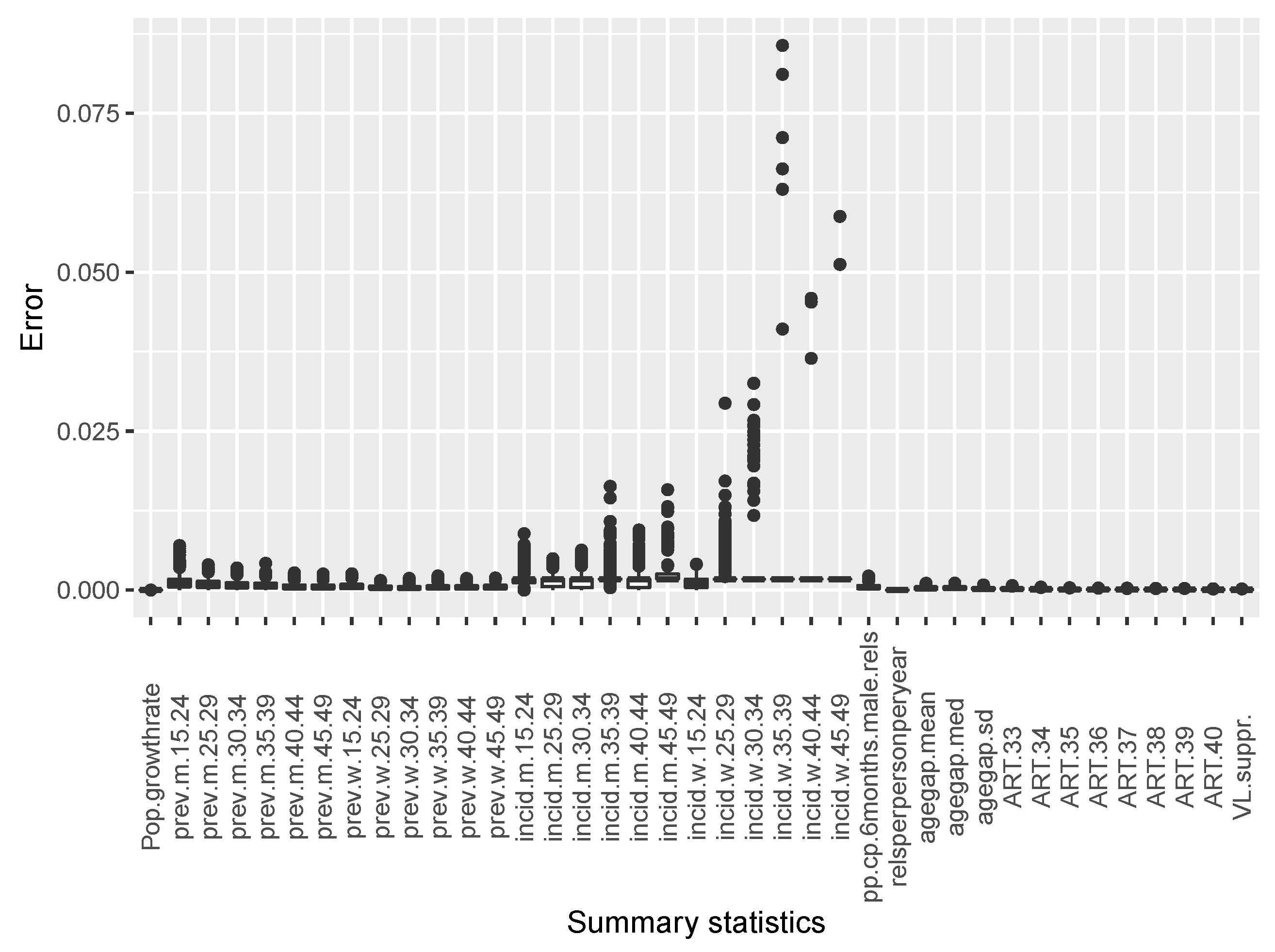
Appendix B.3.1. Summary Features from Epidemiological and Sexual Behaviour Data

For the first calibration scenario, we calibrated the default modelling framework by using summary features from epidemiological and sexual behaviour data. Explicitly, the summary features values are given in the table below.
Table A5. Mean values of epidemiological and behavioural summary features from benchmark data.
ParameterValue
Demographic
Population growth rate0.97933
HIV epidemiology & ART intervention
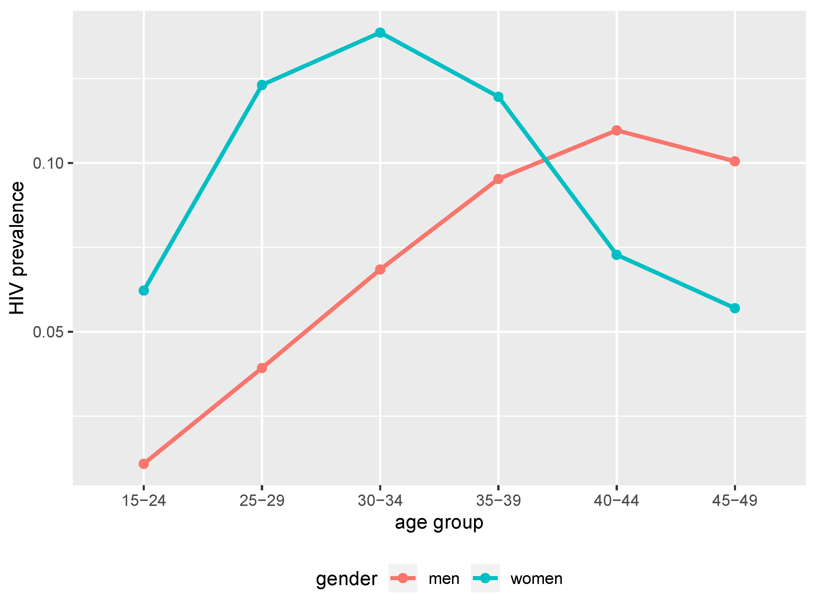
Prevalence for men aged between 15 and 24 years0.0113
Prevalence for men aged between 25 and 29 years0.04081
Prevalence for men aged between 30 and 34 years0.07115
Prevalence for men aged between 35 and 39 years0.09903
Prevalence for men aged between 40 and 44 years0.114
Prevalence for men aged between 45 and 49 years0.10446
Prevalence for women aged between 15 and 24 years0.06467
Prevalence for women aged between 25 and 29 years0.12797
Prevalence for women aged between 30 and 34 years0.14411
Prevalence for women aged between 35 and 39 years0.1243
Prevalence for women aged between 40 and 44 years0.07557
Prevalence for women aged between 45 and 49 years0.05917
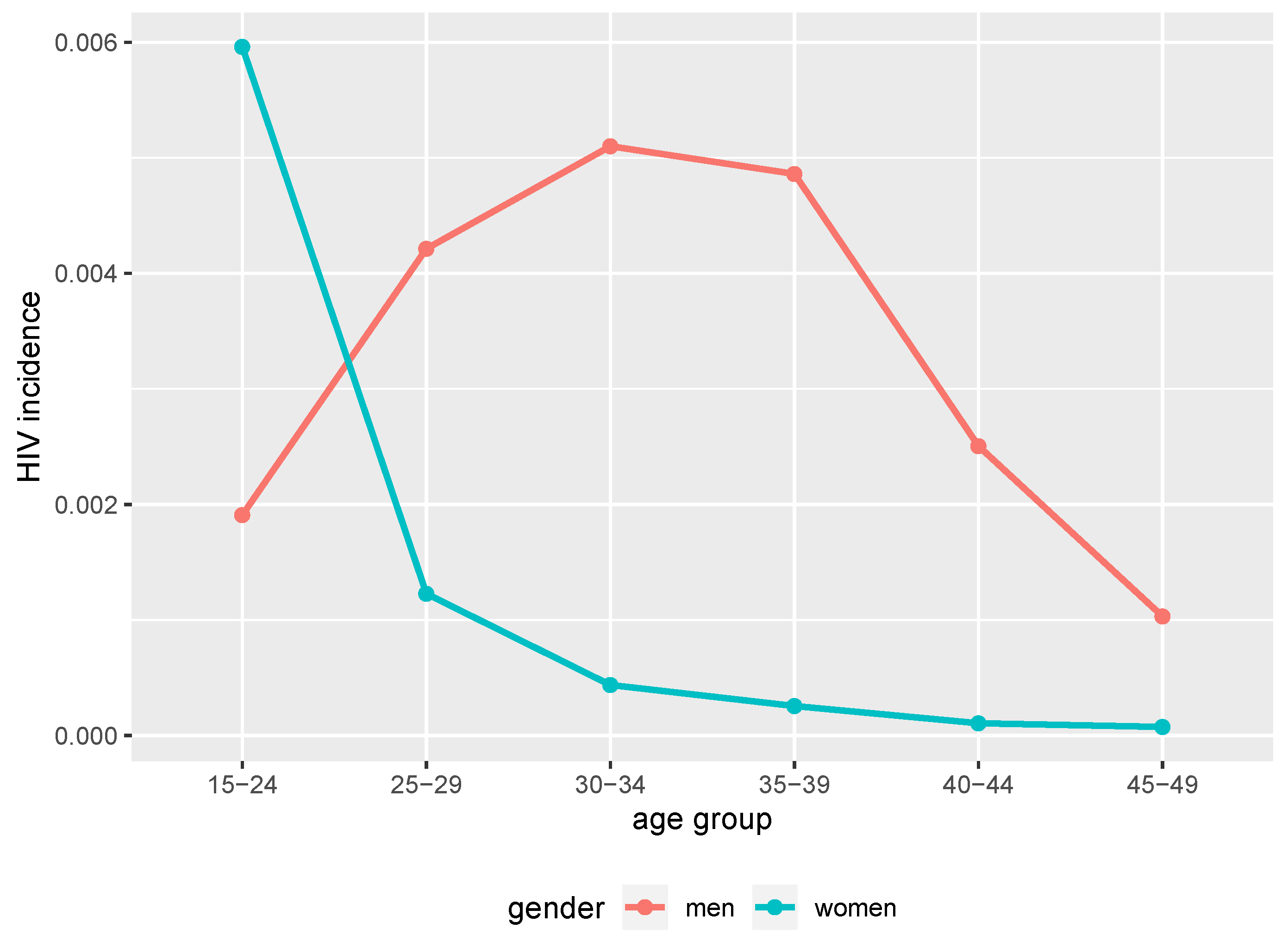
Incidence for men aged between 15 and 24 years0.00198
Incidence for men aged between 25 and 29 years0.00438
Incidence for men aged between 30 and 34 years0.0053
Incidence for men aged between 35 and 39 years0.00505
Incidence for men aged between 40 and 44 years0.0026
Incidence for men aged between 45 and 49 years0.00107
Incidence for women aged between 15 and 24 years0.00619
Incidence for women aged between 25 and 29 years0.00128
Incidence for women aged between 30 and 34 years0.00045
Incidence for women aged between 35 and 39 years0.00027
Incidence for women aged between 40 and 44 years0.00011
Incidence for women aged between 45 and 49 years0.00008
Antiretrovial treatment coverage at 33 years of simulation time0.30333
Antiretrovial treatment coverage at 34 years of simulation time0.42936
Antiretrovial treatment coverage at 35 years of simulation time0.46119
Antiretrovial treatment coverage at 36 years of simulation time0.48869
Antiretrovial treatment coverage at 37 years of simulation time0.61132
Antiretrovial treatment coverage at 38 years of simulation time0.64089
Antiretrovial treatment coverage at 39 years of simulation time0.66607
Antiretrovial treatment coverage at 40 years of simulation time0.79465
Viral suppression0.84
Sexual behaviour
Point prevalence of concurrent partnerships for men0.01935
Average number of relationships per person per year0.4
Mean of age gap14.91719
Median of age gap15.28017
Standard deviation of age gap6.76228
We computed the relative error between mean values of epidemiological and behavioural summary features from benchmark data, and those associated to obtained parameter values in calibration as we can see in Figure A2.
Figure A2. Relative error between mean the value of epi-behavioural benchmark summary features and those associated to retained parameter values during calibration.
Mathematics 09 02645 g0a2

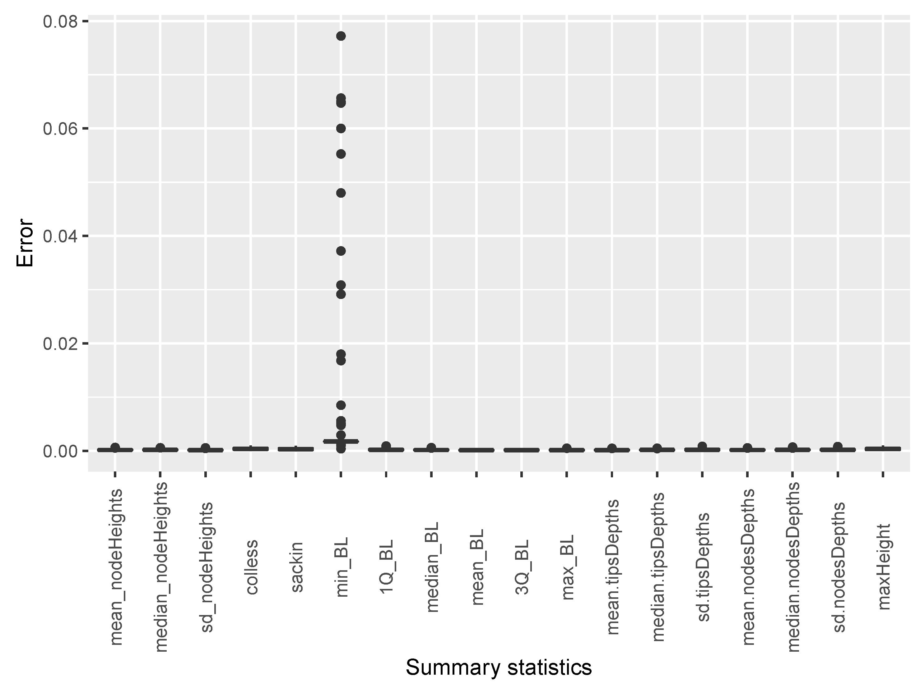
Appendix B.3.2. Summary Features from Phylogenetic Tree Data

For the second calibration scenario, we calibrated the default modelling framework by using summary features from phylogenetic tree data. Explicitly, the summary feature values are given in the table below.
Table A6. Mean values of phylogenetic tree summary features from benchmark data.
ParameterValue
Phylogenetic tree topology
Mean of node heights14.26082
Median of node heights15.38992
Standard deviation of node heights5.96359
Colless index0.08942
Sackin index0.13846
Mean for tips’ depths13.55503
Median for tips’ depths13.26482
Standard deviation for tips’ depths5.26124
Mean for nodes’ depths11.62515
Median for nodes’ depths11.34367
Standard deviation for nodes’ depths5.38234
Phylogenetic tree branch length
Minimum value of branch length0.00105
First quantile of branch length0.69956
Median value of branch length2.33402
Mean value of branch length3.87808
Third quantile of branch length5.50728
Maximum value of branch length20.1533
Maximum Height0.13391
We computed the relative error between mean values of phylogenetic tree summary features from benchmark data, and those associated to obtained parameter values in calibration as we can see in Figure A3.
Figure A3. Relative error between mean the value of the benchmark phylogenetic tree’s summary features and those associated to retained parameter values during calibration.
Mathematics 09 02645 g0a3

Appendix B.3.3. Combined Summary Features

For the third calibration scenario, we calibrated the default modelling framework by using summary features from epidemiological and behavioural data and phylogenetic tree data. We took the summary features values given in Table A5 and Table A6. The trend of the relative error between mean values of combined summary features from benchmark data, and those obtained in calibration is shown in Figure A4.
Figure A4. Relative error between mean values of a combination of epi-behavioural and the phylogenetic tree’s summary features and those associated to retained parameter values during calibration.
Mathematics 09 02645 g0a4
We computed the relative error between mean values of epidemiological and behavioural, and phylogenetic tree summary features from benchmark data, and those associated to the obtained parameter values in calibration as we can see in Figure A4, which is a combination of Figure A2 and Figure A3.

References

  1. Fettig, J.; Swaminathan, M.; Murrill, C.S.; Kaplan, J.E. Global epidemiology of HIV. Infect. Dis. Clin. 2014, 28, 323–337. [Google Scholar] [CrossRef] [Green Version]
  2. Kharsany, A.B.; Karim, Q.A. HIV infection and AIDS in sub-Saharan Africa: Current status, challenges and opportunities. Open AIDS J. 2016, 10, 34. [Google Scholar] [CrossRef] [Green Version]
  3. Ward, H.; Rönn, M. The contribution of STIs to the sexual transmission of HIV. Curr. Opin. HIV AIDS 2010, 5, 305. [Google Scholar] [CrossRef] [Green Version]
  4. Fox, A.M. The social determinants of HIV serostatus in sub-Saharan Africa: An inverse relationship between poverty and HIV? Public Health Rep. 2010, 125, 16–24. [Google Scholar] [CrossRef] [PubMed] [Green Version]
  5. Kalichman, S.C.; Ntseane, D.; Nthomang, K.; Segwabe, M.; Phorano, O.; Simbayi, L.C. Recent multiple sexual partners and HIV transmission risks among people living with HIV/AIDS in Botswana. Sex. Transm. Infect. 2007, 83, 371–375. [Google Scholar] [CrossRef] [Green Version]
  6. Mah, T.L.; Halperin, D.T. Concurrent sexual partnerships and the HIV epidemics in Africa: Evidence to move forward. AIDS Behav. 2010, 14, 11–16. [Google Scholar] [CrossRef] [PubMed] [Green Version]
  7. Hunter, D.J. AIDS in sub-Saharan Africa: The epidemiology of heterosexual transmission and the prospects for prevention. Epidemiology 1993, 4, 63–72. [Google Scholar] [CrossRef] [PubMed]
  8. Shang, Y. Modeling epidemic spread with awareness and heterogeneous transmission rates in networks. J. Biol. Phys. 2013, 39, 489–500. [Google Scholar] [CrossRef] [Green Version]
  9. Beauclair, R. Age Differences in Sexual Relationships and HIV Transmission: Statistical Analyses of Bio-Behavioural Survey Data from Southern Africa. Ph.D. Thesis, Ghent University, Ghent, Belgium, 2018. [Google Scholar]
  10. Nelson, K.E.; Galai, N.; Safaeian, M.; Strathdee, S.A.; Celentano, D.D.; Vlahov, D. Temporal trends in the incidence of human immunodeficiency virus infection and risk behavior among injection drug users in Baltimore, Maryland, 1988–1998. Am. J. Epidemiol. 2002, 156, 641–653. [Google Scholar] [CrossRef] [Green Version]
  11. Grabowski, M.K.; Serwadda, D.M.; Gray, R.H.; Nakigozi, G.; Kigozi, G.; Kagaayi, J.; Ssekubugu, R.; Nalugoda, F.; Lessler, J.; Lutalo, T.; et al. HIV prevention efforts and incidence of HIV in Uganda. N. Engl. J. Med. 2017, 377, 2154–2166. [Google Scholar] [CrossRef]
  12. Riedner, G.; Hoffmann, O.; Rusizoka, M.; Mmbando, D.; Maboko, L.; Grosskurth, H.; Todd, J.; Hayes, R.; Hoelscher, M. Decline in sexually transmitted infection prevalence and HIV incidence in female barworkers attending prevention and care services in Mbeya Region, Tanzania. Aids 2006, 20, 609–615. [Google Scholar] [CrossRef] [PubMed]
  13. Smith, J.; Nyamukapa, C.; Gregson, S.; Lewis, J.; Magutshwa, S.; Schumacher, C.; Mushati, P.; Hallett, T.; Garnett, G. The distribution of sex acts and condom use within partnerships in a rural sub-Saharan African population. PLoS ONE 2014, 9, e88378. [Google Scholar] [CrossRef] [PubMed] [Green Version]
  14. Hazelbag, C.M.; Dushoff, J.; Dominic, E.M.; Mthombothi, Z.E.; Delva, W. Calibration of individual-based models to epidemiological data: A systematic review. PLoS Comput. Biol. 2020, 16, e1007893. [Google Scholar] [CrossRef] [PubMed]
  15. Helleringer, S.; Kohler, H.P. Sexual network structure and the spread of HIV in Africa: Evidence from Likoma Island, Malawi. Aids 2007, 21, 2323–2332. [Google Scholar] [CrossRef] [PubMed]
  16. Helleringer, S.; Mkandawire, J.; Kalilani-Phiri, L.; Kohler, H.P. Cohort profile: The Likoma network study (LNS). Int. J. Epidemiol. 2014, 43, 545–557. [Google Scholar] [CrossRef] [Green Version]
  17. Grabowski, M.K.; Redd, A.D. Molecular tools for studying HIV transmission in sexual networks. Curr. Opin. HIV AIDS 2014, 9, 126. [Google Scholar] [CrossRef]
  18. De Oliveira, T.; Kharsany, A.B.; Gräf, T.; Cawood, C.; Khanyile, D.; Grobler, A.; Puren, A.; Madurai, S.; Baxter, C.; Karim, Q.A.; et al. Transmission networks and risk of HIV infection in KwaZulu-Natal, South Africa: A community-wide phylogenetic study. Lancet HIV 2017, 4, e41–e50. [Google Scholar] [CrossRef] [Green Version]
  19. Robinson, K.; Fyson, N.; Cohen, T.; Fraser, C.; Colijn, C. How the dynamics and structure of sexual contact networks shape pathogen phylogenies. PLoS Comput. Biol. 2013, 9, e1003105. [Google Scholar] [CrossRef]
  20. Leigh Brown, A.J.; Lycett, S.J.; Weinert, L.; Hughes, G.J.; Fearnhill, E.; Dunn, D.T. Transmission network parameters estimated from HIV sequences for a nationwide epidemic. J. Infect. Dis. 2011, 204, 1463–1469. [Google Scholar] [CrossRef] [Green Version]
  21. Baum, D. Reading a phylogenetic tree: The meaning of monophyletic groups. Nat. Educ. 2008, 1, 190. [Google Scholar]
  22. Stadler, T.; Kühnert, D.; Bonhoeffer, S.; Drummond, A.J. Birth–death skyline plot reveals temporal changes of epidemic spread in HIV and hepatitis C virus (HCV). Proc. Natl. Acad. Sci. USA 2013, 110, 228–233. [Google Scholar] [CrossRef] [Green Version]
  23. Grabowski, M.K.; Lessler, J.; Redd, A.D.; Kagaayi, J.; Laeyendecker, O.; Ndyanabo, A.; Nelson, M.I.; Cummings, D.A.; Bwanika, J.B.; Mueller, A.C.; et al. The role of viral introductions in sustaining community-based HIV epidemics in rural Uganda: Evidence from spatial clustering, phylogenetics, and egocentric transmission models. PLoS Med. 2014, 11, e1001610. [Google Scholar] [CrossRef] [PubMed] [Green Version]
  24. Hallinan, N. Tree shape: Phylogenies & macroevolution. Integr. Biol. B 2011, 9. Available online: http://ib.berkeley.edu/courses/ib200b/lect/ib200b_lect16_Nat_Hallinan_Lindberg_tree_shape2.pdf (accessed on 10 July 2020).
  25. Colijn, C.; Gardy, J. Phylogenetic tree shapes resolve disease transmission patterns. Evol. Med. Public Health 2014, 2014, 96–108. [Google Scholar] [CrossRef] [PubMed]
  26. Giardina, F.; Romero-Severson, E.O.; Albert, J.; Britton, T.; Leitner, T. Inference of transmission network structure from HIV phylogenetic trees. PLoS Comput. Biol. 2017, 13, e1005316. [Google Scholar] [CrossRef] [Green Version]
  27. Lewis, F.; Hughes, G.J.; Rambaut, A.; Pozniak, A.; Brown, A.J.L. Episodic sexual transmission of HIV revealed by molecular phylodynamics. PLoS Med. 2008, 5, e50. [Google Scholar] [CrossRef] [Green Version]
  28. Volz, E.M.; Pond, S.L.K.; Ward, M.J.; Brown, A.J.L.; Frost, S.D. Phylodynamics of infectious disease epidemics. Genetics 2009, 183, 1421–1430. [Google Scholar] [CrossRef] [Green Version]
  29. Rasmussen, D.A.; Volz, E.M.; Koelle, K. Phylodynamic inference for structured epidemiological models. PLoS Comput. Biol. 2014, 10, e1003570. [Google Scholar] [CrossRef]
  30. Liesenborgs, J.; Hendrickx, D.M.; Kuylen, E.; Niyukuri, D.; Hens, N.; Delva, W. SimpactCyan 1.0: An Open-source Simulator for Individual-Based Models in HIV Epidemiology with R and Python Interfaces. Sci. Rep. 2019, 9, 1–13. [Google Scholar] [CrossRef] [Green Version]
  31. Vasylyeva, T.I.; Friedman, S.R.; Paraskevis, D.; Magiorkinis, G. Integrating molecular epidemiology and social network analysis to study infectious diseases: Towards a socio-molecular era for public health. Infect. Genet. Evol. 2016, 46, 248–255. [Google Scholar] [CrossRef] [Green Version]
  32. Paraskevis, D.; Nikolopoulos, G.; Magiorkinis, G.; Hodges-Mameletzis, I.; Hatzakis, A. The application of HIV molecular epidemiology to public health. Infect. Genet. Evol. 2016, 46, 159–168. [Google Scholar] [CrossRef] [PubMed]
  33. Grenfell, B.T.; Pybus, O.G.; Gog, J.R.; Wood, J.L.; Daly, J.M.; Mumford, J.A.; Holmes, E.C. Unifying the epidemiological and evolutionary dynamics of pathogens. Science 2004, 303, 327–332. [Google Scholar] [CrossRef] [Green Version]
  34. Niyukuri, D.; Nyasulu, P.; Delva, W. Assessing the uncertainty around age-mixing patterns in HIV transmission inferred from phylogenetic trees. PLoS ONE 2021, 16, e0249013. [Google Scholar] [CrossRef]
  35. Liesenborgs, J. Simpact Cyan. 2017. Available online: https://simpactcyan.readthedocs.io/en/latest/index.html (accessed on 10 July 2020).
  36. Plazy, M.; Dabis, F.; Naidu, K.; Joanna, O.G.; Barnighausen, T.; Rosemary, D.S. Change of treatment guidelines and evolution of ART initiation in rural South Africa: Data of a large HIV care and treatment programme. BMC Infect. Dis. 2015, 15, 1–8. [Google Scholar] [CrossRef] [Green Version]
  37. Tymejczyk, O.; Brazier, E.; Yiannoutsos, C.; Wools-Kaloustian, K.; Althoff, K.; Crabtree-Ramírez, B.; Van Nguyen, K.; Zaniewski, E.; Dabis, F.; Sinayobye, J.d.; et al. HIV treatment eligibility expansion and timely antiretroviral treatment initiation following enrollment in HIV care: A metaregression analysis of programmatic data from 22 countries. PLoS Med. 2018, 15, e1002534. [Google Scholar] [CrossRef] [PubMed] [Green Version]
  38. Zuma, K.; Shisana, O.; Rehle, T.M.; Simbayi, L.C.; Jooste, S.; Zungu, N.; Labadarios, D.; Onoya, D.; Evans, M.; Moyo, S.; et al. New insights into HIV epidemic in South Africa: Key findings from the National HIV Prevalence, Incidence and Behaviour Survey, 2012. Afr. J. AIDS Res. 2016, 15, 67–75. [Google Scholar] [CrossRef]
  39. Bicego, G.T.; Nkambule, R.; Peterson, I.; Reed, J.; Donnell, D.; Ginindza, H.; Duong, Y.T.; Patel, H.; Bock, N.; Philip, N.; et al. Recent patterns in population-based HIV prevalence in Swaziland. PLoS ONE 2013, 8, e77101. [Google Scholar]
  40. Justman, J.; Reed, J.B.; Bicego, G.; Donnell, D.; Li, K.; Bock, N.; Koler, A.; Philip, N.M.; Mlambo, C.K.; Parekh, B.S.; et al. Swaziland HIV Incidence Measurement Survey (SHIMS): A prospective national cohort study. Lancet HIV 2017, 4, e83–e92. [Google Scholar] [CrossRef] [Green Version]
  41. Rambaut, A.; Grass, N.C. Seq-Gen: An application for the Monte Carlo simulation of DNA sequence evolution along phylogenetic trees. Bioinformatics 1997, 13, 235–238. [Google Scholar] [CrossRef]
  42. West, B.T.; Welch, K.B.; Galecki, A.T. Linear Mixed Models: A Practical Guide Using Statistical Software; CRC Press: Boca Raton, FL, USA, 2014. [Google Scholar]
  43. Bates, D.; Mächler, M.; Bolker, B.; Walker, S. Fitting linear mixed-effects models using lme4. arXiv 2014, arXiv:1406.5823. [Google Scholar]
  44. Stein, M. Large sample properties of simulations using Latin hypercube sampling. Technometrics 1987, 29, 143–151. [Google Scholar] [CrossRef]
  45. McKay, M.D.; Beckman, R.J.; Conover, W.J. A comparison of three methods for selecting values of input variables in the analysis of output from a computer code. Technometrics 2000, 42, 55–61. [Google Scholar] [CrossRef]
  46. Csilléry, K.; Blum, M.G.; Gaggiotti, O.E.; François, O. Approximate Bayesian computation (ABC) in practice. Trends Ecol. Evol. 2010, 25, 410–418. [Google Scholar] [CrossRef]
  47. Akullian, A.; Bershteyn, A.; Klein, D.; Vandormael, A.; Bärnighausen, T.; Tanser, F. Sexual partnership age pairings and risk of HIV acquisition in rural South Africa. AIDS 2017, 31, 1755. [Google Scholar] [CrossRef] [PubMed]
  48. Cohen, M.S.; Chen, Y.Q.; McCauley, M.; Gamble, T.; Hosseinipour, M.C.; Kumarasamy, N.; Hakim, J.G.; Kumwenda, J.; Grinsztejn, B.; Pilotto, J.H.; et al. Prevention of HIV-1 infection with early antiretroviral therapy. N. Engl. J. Med. 2011, 365, 493–505. [Google Scholar] [CrossRef] [PubMed] [Green Version]
  49. Willem, L. Agent-Based Models for Infectious Disease Transmission: Exploration, Estimation & Computational Efficiency. Ph.D. Thesis, University of Antwerp, Antwerp, Belgium, 2015. [Google Scholar]
  50. Hunter, E.; Mac Namee, B.; Kelleher, J.D. A Comparison of Agent-Based Models and Equation Based Models for Infectious Disease Epidemiology. In Proceedings of the 26th AIAI Irish Conference on Artificial Intelligence and Cognitive Science, Dublin, Ireland, 6–7 December 2018. [Google Scholar]
  51. Shang, Y. Mixed SI (R) epidemic dynamics in random graphs with general degree distributions. Appl. Math. Comput. 2013, 219, 5042–5048. [Google Scholar] [CrossRef]
  52. Arnaout, R.A.; Lloyd, A.L.; O’Brien, T.R.; Goedert, J.J.; Leonard, J.M.; Nowak, M.A. A simple relationship between viral load and survival time in HIV-1 infection. Proc. Natl. Acad. Sci. USA 1999, 96, 11549–11553. [Google Scholar] [CrossRef] [Green Version]
  53. Leventhal, M.G.E. An R package ‘expoTree’, r2013. Available online: http://www2.uaem.mx/r-mirror/web/packages/expoTree/expoTree.pdf (accessed on 7 July 2020).
  54. Revell, L.J. phytools: An R package for phylogenetic comparative biology (and other things). Methods Ecol. Evol. 2012, 3, 217–223. [Google Scholar] [CrossRef]
  55. LANL. HIV-1 Subtype C. 2017. Available online: https://www.hiv.lanl.gov/components/sequence/HIV/asearch/query_one.comp?se_id=JN188292 (accessed on 7 July 2020).
  56. LANL. Landmarks of the HIV-1 Genome. 2017. Available online: https://www.hiv.lanl.gov/content/sequence/HIV/MAP/landmark.html (accessed on 7 July 2020).
  57. Darriba, D.; Posada, D. jModelTest 2 Manual v0. 1.10. Parallel Comput. 2016, 9, 772. [Google Scholar]
  58. Lemey, P.; Rambaut, A.; Pybus, O.G. HIV evolutionary dynamics within and among hosts. AIDS Rev. 2006, 8, 125–140. [Google Scholar]
  59. Frost, S.D.; Pybus, O.G.; Gog, J.R.; Viboud, C.; Bonhoeffer, S.; Bedford, T. Eight challenges in phylodynamic inference. Epidemics 2015, 10, 88–92. [Google Scholar] [CrossRef] [Green Version]
  60. Metcalf, C.; Birger, R.; Funk, S.; Kouyos, R.; Lloyd-Smith, J.; Jansen, V. Five challenges in evolution and infectious diseases. Epidemics 2015, 10, 40–44. [Google Scholar] [CrossRef] [PubMed] [Green Version]
  61. Gog, J.R.; Pellis, L.; Wood, J.L.; McLean, A.R.; Arinaminpathy, N.; Lloyd-Smith, J.O. Seven challenges in modeling pathogen dynamics within-host and across scales. Epidemics 2015, 10, 45–48. [Google Scholar] [CrossRef] [PubMed] [Green Version]
  62. Volz, E.M.; Romero-Severson, E.; Leitner, T. Phylodynamic inference across epidemic scales. Mol. Biol. Evol. 2017, 34, 1276–1288. [Google Scholar] [CrossRef] [Green Version]
  63. Mideo, N.; Alizon, S.; Day, T. Linking within-and between-host dynamics in the evolutionary epidemiology of infectious diseases. Trends Ecol. Evol. 2008, 23, 511–517. [Google Scholar] [CrossRef] [PubMed]
Figure 1. HIV point prevalence at 40 years of simulation time from the simulated epidemic. Age and gender structured point prevalence from benchmark data (2017 in calendar time).
Mathematics 09 02645 g001
Figure 2. HIV incidence in 35–40 simulation time from the simulated epidemic. Age and gender structured incidence at 40 years of simulation time from benchmark data (2017 in calendar time).
Mathematics 09 02645 g002
Figure 3. Work-flow with the main steps for the calibration simulation study. The first step is to generate the benchmark data set with selected parameter values. The second step is the calibration of the default modelling framework. The third step is to run the modelling framework using retained parameter values from calibration.
Mathematics 09 02645 g003
Figure 4. Temporal trends of HIV incidence produced by vectors of retained parameter values. Incidence values from benchmark data and after calibration when the simulation was performed by vectors of retained parameters. (Combined features—2nd column, epidemiological and behavioural features—3rd column, and phylogenetic features—4th column).
Mathematics 09 02645 g004
Figure 5. Temporal trends of HIV incidence produced by median values of retained parameter values. Incidence values in different age groups from benchmark data and after calibration when the simulation was performed by median values of the retained parameters. (Combined features—2nd column, epidemiological and behavioural features—3rd column, and phylogenetic features—4th column).
Mathematics 09 02645 g005
Table 1. Mean values for estimates of age-mixing patterns in sexual partnerships from the master model and after calibration with features from HIV epidemiology and sexual behaviour (Calibration 1), phylogenetic tree (Calibration 2), and a combination of the two types of features (Calibration 3).
EstimateBenchmarkCalibration 1Calibration 1 *Calibration 2Calibration 2 *Calibration 3Calibration 3 *
AAD13.78213.86114.16713.15113.11113.63313.83
SDAD6.156.1146.176.0086.1136.0736.164
BSD2.1382.0132.0772.0262.1372.0042.098
WSD1.8121.7811.7741.8371.8071.8111.779
Slope0.3150.2970.3020.3160.3190.3050.305
Intercept−2.378−2.111−2.336−2.099−2.2−2.164−2.264
* Values computed when we run the simulation with medians of the retained parameter values during calibration.
Table 2. Mean relative error for the average of age mixing estimates compared between benchmark data and after calibration with features from HIV epidemiology and sexual behaviour (MRE 1), a phylogenetic tree (MRE 2), and a combination of the two types of features (MRE 3).
EstimateMRE 1MRE 1 *MRE 2MRE 2 *MRE 3MRE 3 *
AAD0.163990.039480.192380.051770.167660.0325
SDAD0.102480.041450.104470.040050.103670.04208
BSD0.173730.069070.160630.062540.162580.06986
WSD0.099650.0570.109250.053680.101930.05984
Slope0.205580.083950.219150.073150.204820.07606
Intercept0.370340.163610.391380.165110.399990.16004
* Error obtained when we run the simulation with medians of the retained parameter values during calibration.
Table 3. Mean values for estimates of HIV onward transmissions from the master model and after calibration with features from HIV epidemiology and sexual behaviour (Calibration 1), a phylogenetic tree (Calibration 2), and a combination of the two types of features (Calibration 3).
EstimateBenchmarkCalibration 1Calibration 1 *Calibration 2Calibration 2 *Calibration 3Calibration 3 *
Mean2.2422.3842.2452.3232.242.3562.246
Median1.3911.3511.311.3911.3031.3541.337
Standard deviation2.122.6222.272.4282.2962.5792.273
* Values computed when we run the simulation with medians of the retained parameter values during calibration.
Table 4. Mean relative error of average values of onward HIV transmission statistics compared between benchmark data and after calibration with HIV epidemiology and sexual behaviour (MRE 1), a phylogenetic tree (MRE 2), and a combination of the two types of features (MRE 3).
EstimateMRE 1MRE 1 *MRE 2MRE 2 *MRE 3MRE 3 *
Mean0.175130.13490.157160.126860.168070.13272
Median0.32710.319990.341160.319620.325610.32279
Standard deviation0.469320.325610.392350.326760.455390.33333
* Error obtained when we run the simulation with medians of the retained parameter values during calibration.
Table 5. Mean relative error for average incidence values in male populations compared between benchmark data and after calibration with HIV epidemiology and sexual behaviour (MRE 1), phylogenetic tree (MRE 2), and a combination of the two types of features (MRE 3).
YearAge GroupMRE 1MRE 1 *MRE 2MRE 2 *MRE 3MRE 3 *
201315–241.054750.880481.341371.07451.062950.93416
25–290.878110.767120.952020.884610.899380.78916
30–340.916060.88750.968490.919550.960050.88494
35–390.784080.669740.74410.675470.756290.67397
40–440.891730.784560.794730.737470.915720.74142
45–491.231311.040451.130160.992371.227111.00805
201415–241.022930.898831.262961.08511.085330.97876
25–290.962490.886941.102311.026980.989510.90741
30–340.864080.870180.903730.896810.921650.84121
35–390.978270.877330.930420.884250.998370.8737
40–441.069910.910030.920590.916560.977180.88609
45–491.450551.298481.271031.166571.44481.15002
201515–241.158550.895251.334171.253471.270411.03238
25–291.005250.935521.093951.160551.121760.9917
30–340.923420.890380.912070.960750.949960.93358
35–391.074370.933580.954230.900220.907460.87915
40–441.073160.880810.962760.802361.000170.85782
45–491.755761.507131.538881.441271.551751.37258
201615–241.134250.989861.334531.227381.256741.0544
25–291.021550.965231.235361.056841.059840.96505
30–340.919180.943910.979931.031220.971030.97724
35–391.186621.26731.253781.126951.161831.20835
40–441.036650.960060.965480.833960.909250.92091
45–491.470051.410021.405451.299731.388281.31173
201715–241.359791.12091.351271.296331.393861.21792
25–290.958061.012591.088131.014330.990.97441
30–341.004970.978031.089161.015951.024051.00899
35–391.342271.468931.32671.302321.350381.37524
40–441.139721.072221.209090.997361.052621.03022
45–491.587921.512931.745171.388751.478871.41031
* Error obtained when we run the simulation with medians of the retained parameter values during calibration.
Table 6. Mean relative error for average incidence values in the female population compared between benchmark data and after calibration with HIV epidemiology and sexual behaviour (MRE 1), a phylogenetic tree (MRE 2), and a combination of the two types of features (MRE 3).
YearAge GroupMRE 1MRE 1 *MRE 2MRE 2 *MRE 3MRE 3 *
201315–240.531620.478720.529740.496370.496740.46769
25–291.17111.101911.025981.081741.068561.07796
30-341.45541.597381.480931.46741.576721.38211
35–391.273891.569121.434071.451381.47231.39072
40–441.52371.775821.585681.656771.698821.47681
45–491.412141.957961.453111.639711.510471.46651
201415–240.542650.504750.584630.53470.542350.48523
25–291.355381.307141.252421.197491.267111.21816
30–341.587651.741941.512931.544551.595641.3997
35–391.29581.443171.481711.567041.470451.27727
40–441.476261.652271.570111.614471.457991.44798
45–491.517651.75991.517711.57891.495141.36147
201515–240.579550.529970.600270.577680.582390.53849
25–291.518211.571281.530551.492221.590131.42023
30–341.466851.648331.527671.559351.575461.48934
35–391.871221.857791.715331.560981.753731.34148
40–441.525581.720441.538491.807551.465661.42572
45–491.725151.609111.483151.524581.628341.40109
201615–240.587430.601290.618150.625630.598050.60696
25–291.461321.50591.414931.43171.486551.40186
30–341.521391.589941.677281.573461.535131.44627
35–391.673031.888481.780091.901381.918321.4736
40–441.401861.735261.422211.500551.782631.34671
45–491.520932.172042.059121.899811.451321.52321
201715–240.700510.68830.797290.746520.754460.71317
25–291.582321.671521.582251.482881.502271.45087
30–341.873832.078421.770461.91081.870731.54384
35–391.735211.619321.67162.070311.491611.6285
40–441.941662.257491.893541.82691.858431.5933
45–491.269631.619161.247912.06851.327761.45465
* Error obtained when we run the simulation with medians of the retained parameter values during calibration.
Publisher’s Note: MDPI stays neutral with regard to jurisdictional claims in published maps and institutional affiliations.

