
Variable Weight Matter–Element Extension Model for the Stability Classification of Slope Rock Mass


School of Resources and Safety Engineering, Central South University, Changsha 410083, China
*
Author to whom correspondence should be addressed.
Mathematics 2021, 9(21), 2807; https://0-doi-org.brum.beds.ac.uk/10.3390/math9212807
Submission received: 17 September 2021
/
Revised: 20 October 2021
/
Accepted: 26 October 2021
/
Published: 4 November 2021
(This article belongs to the Special Issue Analytical, Numerical and Big-Data-Based Methods in Deep Rock Mechanics)
Abstract
:The slope stability in an open-pit mine is closely related to the production safety and economic benefit of the mine. As a result of the increase in the number and scale of mine slopes, slope instability is frequently encountered in mines. Therefore, it is of scientific and social significance to strengthen the study of the stability of the slope rock mass. To accurately classify the stability of the slope rock mass in an open-pit mine, a new stability evaluation model of the slope rock mass was established based on variable weight and matter–element extension theory. First, based on the main evaluation indexes of geology, the environment, and engineering, the stability evaluation index system of the slope rock mass was constructed using the corresponding classification criteria of the evaluation index. Second, the constant weight of the evaluation index value was calculated using extremum entropy theory, and variable weight theory was used to optimize the constant weight to obtain the variable weight of the evaluation index value. Based on matter–element extension theory, the comprehensive correlation between the upper and lower limit indexes in the classification criteria and each classification was calculated, in addition to the comprehensive correlation between the rock mass indexes and the stability grade of each slope. Finally, the grade variable method was used to calculate the grade variable interval corresponding to the classification criteria of the evaluation index and the grade variable value of each slope rock mass, so as to determine the stability grade of the slope rock. The comparison results showed that the classification results of the proposed model are in line with engineering practice, and more accurate than those of the hierarchical-extension model and the multi-level unascertained measure-set pair analysis model.
1. Introduction
In the mining of an open pit, the stability of the slope rock mass has a significant impact on mining design, intensity, and safety. As a result of the gradual depletion of surface mineral resources, underground mining has been employed instead of open-pit mining in large mines [1,2]. Therefore, it is necessary to study the stability of open-pit slopes. The slope rock mass of open-pit mines is significantly affected by many factors, such as weathering, in situ stress, groundwater, and blasting vibration. There is an urgent need for the accurate determination of the stability grade of the slope rock mass. As a result of the progress of scientific theory and method, the evaluation of the stability of the slope rock mass in open-pit mines has developed from empirical judgment, theoretical analysis, and qualitative evaluation of a single index, to a comprehensive evaluation based on an index system [3,4,5]. In general, three main methods are used to evaluate the stability of the slope rock mass in open-pit mines: (1) solid modeling and numerical simulation methods. By analyzing the influence of the distribution of structural planes (such as joints and fissures) in the slope rock mass on rock anisotropy, Shi Wenhao, Yang Tianhong et al. [6] evaluated the stability of the slope rock mass in an open-pit using a 3D solid modeling method. To determine the stability of the open-pit slope, Zhao Haijun, Ma Fengshan et al. [7] analyzed the surrounding rock of the underground stope, the mechanical environment of the slope, and the movement and deformation of the rock mass using a GPS monitoring network and a 3D numerical simulation. (2) Geological survey and refined analysis. Through a detailed geological survey of the quality components and size of the slope, Du Shigui [8] conducted a refined statistical analysis of the survey results, and finally determined the stability of the slope rock mass based on the cybernetics of the rock mass structure. Neil Bara, Michael Kostadinovskia et al. [9] described the rapid and robust process utilized at BHP Limited for appraising a slope failure at an iron ore mine site in the Pilbara region of Western Australia, using a combination of UAV photogrammetry and 3D slope stability models in less than a shift (i.e., less than 12 h). Fehmi Arikan, Fatih Yoleri et al. [10] conducted a geotechnical assessment of slope stability and collected geological data from sources such as geologic reconnaissance, core logging, topographical surveys, and geomechanical laboratory testing data; in addition, kinematical and two-dimensional limit equilibrium back analyses were performed. (3) Qualitative evaluation and analysis based on the evaluation index system. Wang Xinmin, Kangqian et al. [11] evaluated the stability of the open-pit slope rock mass via the construction of an analytic hierarchy process-extension model. Zhang Xu, Zhou Shaowu et al. [12] evaluated the slope and excavation stability of the open-pit mines by building an entropy weight-set evaluation model. Huangdan and Shi Xiuzhi et al. [13] evaluated the stability of the slope rock mass by constructing a multi-level unascertained measure-set pair analysis model. Liu Leilei, Zhang Shaohe et al. [14] evaluated the stability of the slope rock mass by constructing an AHP-ideal point model. Bar N and Barton N. [15] discussed the applicability of the Q-slope method to slopes ranging from less than 5 m to more than 250 m in height, in both civil and mining engineering projects. Pastor, J.L., Riquelme, A.J., et al. [16] used SMRTool, an open-source software package, to derive a complete and detailed definition of the angular relationship between discontinuity and slope, and clarified the evaluation of SMR parameters.
Among the three methods mentioned above, the first is highly theoretical and accurate for the stability classification of slope rock masses with less complex environmental conditions. Although the second method yields accurate evaluation results, significant amounts of manpower and material resources are required in the field survey. Hence, it is less used in the classification of general slope rock stability. The third method, which is based on a mathematical model and an evaluation index system, has good generality and can be used in the stability classifications of various rock masses. However, the construction of the mathematical model and the selection of an index system need to be further improved. Based on the existing research, an evaluation index system for the stability classification of the slope rock mass in open-pit mines was established in this study. First, the index weight was calculated using variable weight theory to address the unreasonable index weighting caused by ignoring the index change in single- or multi-method weighting. Second, based on the matter–element extension model and the grade variable method, the stability of the slope rock mass in the open-pit mine was evaluated, so as to improve the accuracy of the matter–element extension model in the stability classification of the slope rock mass. Finally, a new classification model of slope rock mass stability was constructed.
2. Basic Principles of the Matter–Element Extension Model
The matter–element extension model is a mathematical model based on matter–element theory and extension mathematics. In this model, the matter element is taken as the basic element to describe objects. The matter element is expressed as the ordered triple R = (S,y,v), where S represents the objects; y represents the feature of objects; and v represents quantities of S about y. S, y, and v are called the three elements of the matter element [17]. Based on extension set theory and decision-making theory, matter–element transformation and the correlation function are used as tools. The extension engineering method can be used to solve the application problems in the fields of management, control, and engineering [18].
2.1. Matter Elements, Classical Domains, and Nodal Domains
If the evaluation object S contains a feature y expressed by v, then S, y, and v constitute the ordered triple R = (S,y,v), and are called matter elements [19]. If the evaluation object S has n features, the corresponding values of features y1, y2 … yn are v1, v2…vn, respectively. Matter elements describing the evaluation object S are recorded as R:
The classical domain of evaluation object S about grade j is recorded as Rj:
The feature section of the evaluation object S is recorded as R0:
where S is the evaluation object; vi is the eigenvalue of the evaluation object; Sj is the evaluation object corresponding to the grade j, j = 1, 2,…, m; yi is the eigenvalue of the evaluation object i, i = 1, 2,…, n; Vji is the eigenvalue range of Sj corresponding to yi, Vij = [aij, bij]; S0 is the evaluation object corresponding to all levels; and V0i is the eigenvalue range of S0 corresponding to yi, V0i = [a0i, b0i].
2.2. Extension Correlation Functions
According to the extension set theory and the definition of extension distance [20], the extension distance equation of the feature yi of the evaluation object S with respect to the stability grade j is expressed as follows:
where vi is the feature i of the object to be evaluated, i = 1, 2,…, n; Vji is the value range of Sj for the feature yi, Vij = [aij, bij]; V0i is the value range of S0 for the feature yi, V0i = [a0i, b0i]; ρ(vi, Vji) is the extension distance of the feature yi for the j-level classical domain; and ρ(vi, Vji) is the extension distance of the feature yi for node region; i = 1, 2, n; n = 1, 2,… m.
If vi ∈ V0i, the specified correlation function [21] is expressed as follows:
where Sj (vi) is the single index correlation degree of the feature yi of the evaluation object S with respect to the grade j, i = 1, 2,… n; j = 1, 2,…, m.
Combining with the feature weight vector W of the evaluation object, the calculation expression of the comprehensive correlation [22] of the evaluation object S with respect to the grade j is as follows:
where wi is the weight coefficient of the evaluation object feature yi; Sj (Vj) is the comprehensive correlation between the evaluation object S and the grade j; Sj (vi) is the single index correlation of the evaluation object S feature yi with respect to the grade j; i = 1, 2,…, n.
2.3. Level Variable Method
According to the level variable method [23,24,25], the calculation expression of the level variable is obtained as follows:
where Sj (Vj) is the comprehensive correlation of the evaluation object S and the grade j; Pj (Vj) is the standardized value of the comprehensive correlation; k is the eigenvalue of the stability grade variable of the evaluation object S; Bs = min{Sj (Vj)}, As = max{Sj (Vj)}; and j = 1, 2,…, m.
3. Extreme Entropy Weighting and Variable Weighting Theory
3.1. Principle of Extreme Entropy Weighting
Extremum entropy method can be performed by the following two steps: (1) process the eigenvalues of the evaluation object without dimension to obtain the identical type of eigenvalue, and (2) determine the feature weight of the evaluation object. The previous research has proved that the extremum entropy method has the best performance compared with other entropy methods, and is also called the optimal entropy method [26]. In this study, extreme entropy is used to determine the feature weights of evaluation objects via the following steps.
- The eigenvalue xij of the evaluation object Xi is obtained by extremum method and transformed into a dimensionless value vij. If the feature xij of the evaluation object xi belongs to the positive type, it is processed by Equation (9). If the feature xij of the evaluation object xi belongs to the reverse type, it is processed by Equation (10) [27]:where xij is the eigenvalue of Xi, Mj is the maximum value of xij; mj is the minimum value of xij; vij is the dimensionless value of xij, i = 1, 2,…, n; j = 1, 2,…, m.
- The dimensionless vij of the evaluation object Xi is normalized:where vij is the dimensionless value of the feature xij; rij is the normalized value of the feature xij; and n is the total number of objects to be evaluated.
- The feature information entropy of evaluation object Xi is calculated as follows:where ej is the feature information entropy of the object Xi to be evaluated; rij is the normalized value of the feature xij, i = 1, 2,…, n; j = 1, 2,…, m; and ej ∈ [0,1].
- The feature weight of evaluation object Xi is calculated as follows:where w0j is the weight of the feature xij; ej is the feature information entropy of the feature xij; and m is the total number of features to be evaluated.
The constant weight vector is W0 = (w01, w02,…, w0m).
3.2. Basic Theory of Variable Weight
As a result of the fixed weight value in the constant weight empowerment, the relative importance of each feature of the evaluation object is only reflected, while the impact of the eigenvalue change of the evaluation object on the feature weight is ignored [28]. For this reason, Wang Peizhuang, Li Hongxing et al. proposed and improved the variable weight theory [29]. According to variable weight theory, the constant weight of the evaluation object can be optimized by constructing the variable weight vector to obtain the variable weight of the evaluation object. According to the axiomatic system of the variable weight vector, the variable weight vector is defined as follows [30]:
In the following mapping P: [0,1]m → [0,1]m; X → P(X) = (P1(X); and P2(X),…, Pm(X)); then P is called eigenvariable weight vector. If P is satisfied by (1) punitiality, xi ≥ xj ⇒ Pi(X) ≤ Pj(X); (2) continuity, Pi(X) is continuous for each variable (i = 1, 2,…, n) for any constant weight vector; (3) for any constant weight vector, W0 = (w01, w02,…, w0m); then Equation (14) is satisfied by ① polarity, (w01 + w02 + … +w0m = 1); ② continuity, w0j (x1, x2,…, xm) is continuous with respect to each variable xj (j = 1, 2,…, m); ③ punitiveness, w0j (x1, x2,…, xm) is reduced with respect to the variable xj (j = 1, 2,…,m). Then, P is called penalty contingency vector.
where is the Hardarmard product [31], and W(X) is the variable weight vector of the evaluation object X.
Subsequently, the definition changes to the following: (1) punitiveness xi ≥ xj ⇒ Pi(X) ≤ Pj(X) is changed to incentive xi ≥ xj ⇒ Pi(X) ≥ Pj(X); (3) ③ punitiveness W0 = (w01, w02,…, w0m) with a single reduction of (j = 1, 2,…, m). Regarding the variable xj, it is changed into incentive w0j(x1, x2,…, xm) with the single increase (j = 1, 2,…, m) regarding the variable xj. Then, P is called incentive contingency vector.
The eigenvariable weight vector is essentially a gradient vector of the m-dimensional real function (also known as equilibrium function) [32]. Its calculation formula is as follows:
According to Equations (14) and (15), the variable weight vector W(X) of the evaluation object can be obtained.
4. Establishment of Variable Weight Matter–Element Extension Model for Slope Rock Mass Stability Classification
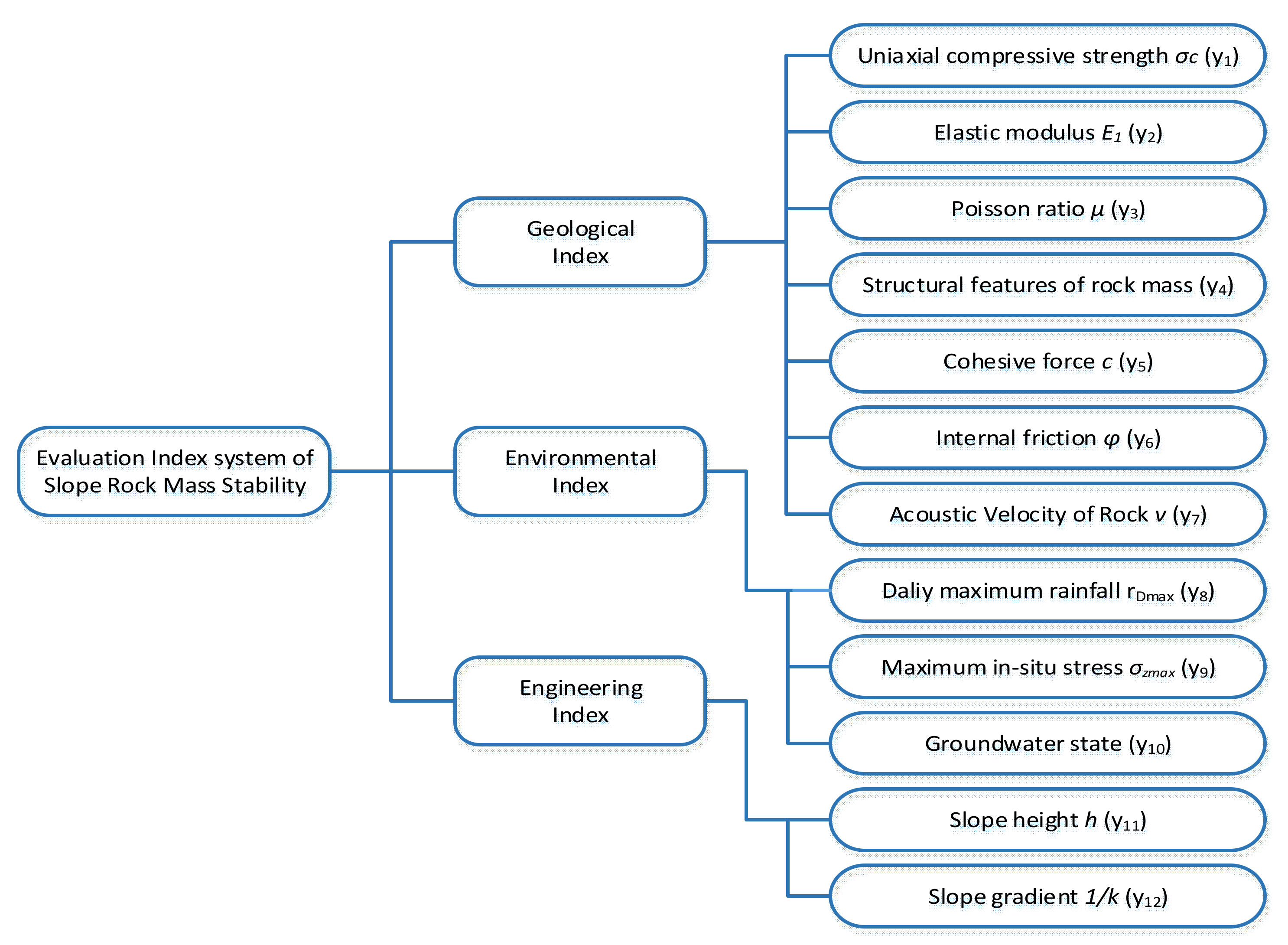
There are many factors affecting the stability of slope rock masses. Establishing a scientific and reasonable evaluation index system is the premise for the accurate evaluation of the slope rock mass stability. The safety evaluation of the slope stability is a dynamic system engineering. The establishment of an evaluation index system is the basic work of evaluation, and the rationality of the evaluation index system directly affects the accuracy of evaluation results. The principle of selecting evaluation indicators is to reflect the most important and comprehensive information with least indicators. Referring to the engineering rock mass classification standard [33,34], the hydroelectric engineering geological survey standard [35], and other researches on the classification criteria of the slope stability and safety evaluation indexes [11,13,36], the geological, environmental, and engineering conditions of the slope rock mass are considered comprehensively in this study. A classification evaluation index system of the slope rock mass stability is constructed by evaluation indexes, such as uniaxial compressive strength; elastic modulus; Poisson’s ratio; structural features; cohesion; internal friction angle; daily maximum rainfall; maximum in situ stress; groundwater state; slope gradient; slope height; and rock acoustic velocity, as shown in Figure 1.
In this study, the classification criteria of the slope rock mass stability evaluation indexes in references [11,13] are employed, as shown in Table 1. Equations (9) and (10) are used to normalize the values in the classification criteria of evaluation indexes, and the classical domain Rj and the nodal domain R0 of the classification criteria of the slope rock mass stability are obtained.
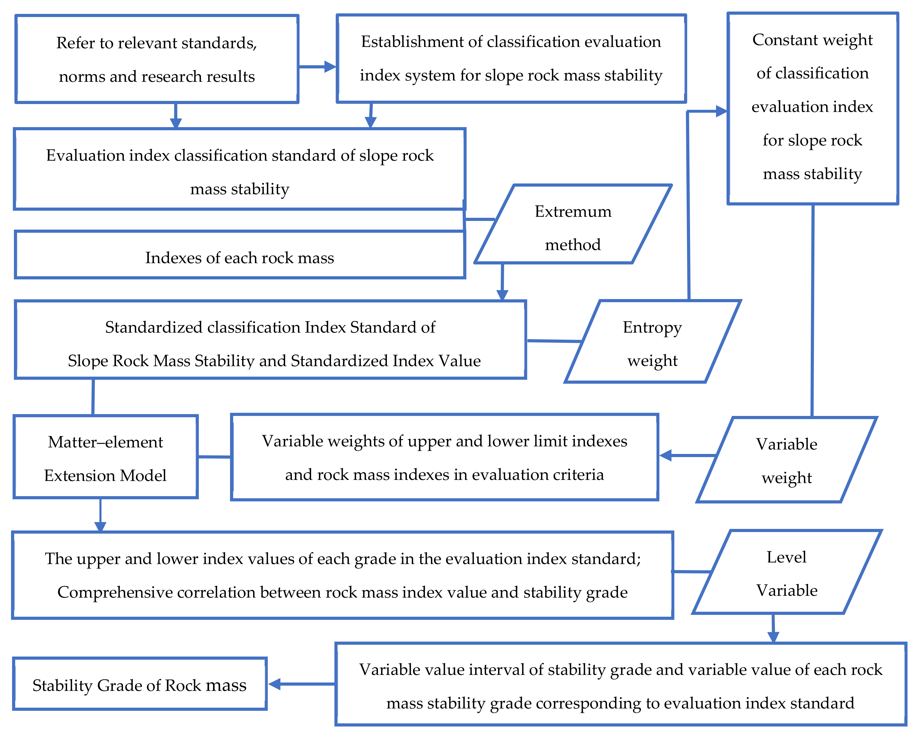
The classical domain Rj expresses the variation range of the standardized index values of the slope rock mass stability evaluation index in each stability grade, and the joint domain R0 expresses the entire range of the standardized index values of the slope rock mass stability classification. Figure 2 shows the calculation process of the rock mass stability classification evaluation using the variable weight matter–element extension model.
5. Case Study in a Mining Project
According to the previous studies [13], the slope rock mass of an open-pit copper mine was formed in 2008. To date, only a part of the slope has been maintained, and the entire slope has remained stable. The evaluation indexes of the slope rock mass were measured and presented in the first four groups of data in Table 2. The data in the fifth group of Table 2 are the slope data of an open-pit mine, presented in previous studies [11]. The actual situation of the slope rock mass was extremely stable. Based on the measured data of slope rock masses in these two mines, the stability of the slope rock masses was evaluated by the proposed model to verify its validity.
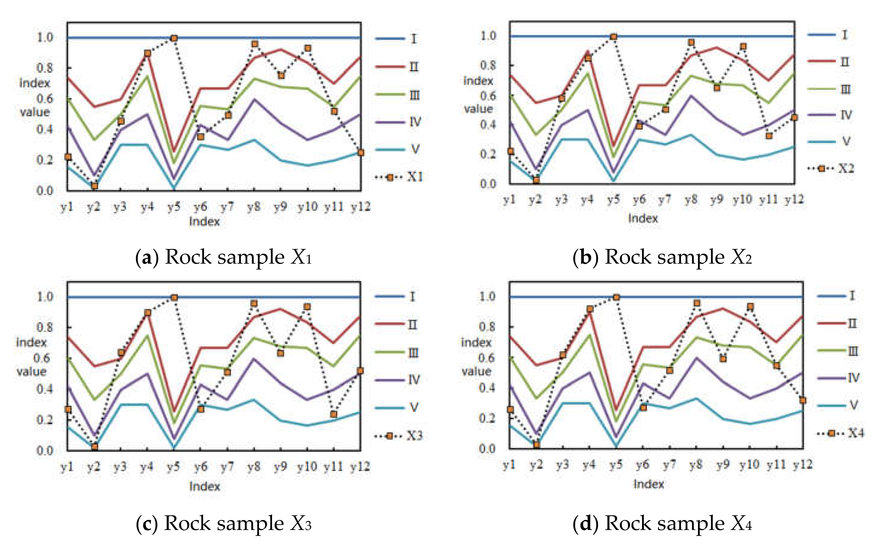
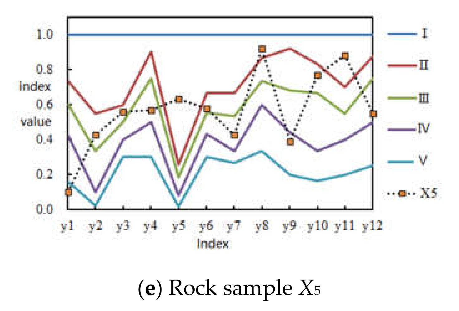
According to Equations (9) and (10), the dimensionless classification index of the slope rock mass is processed. Table 3 presents the dimensionless unified classification indexes. The indexes of five rock mass samples in Table 3 are compared with the evaluation indexes in the classification criteria of the slope rock mass stability, as shown in Figure 3. The solid broken line is connected by the upper limit indexes of each stability grade in the standardized classification criteria of the slope rock mass stability evaluation indexes, and the virtual broken line is connected by the indexes of each rock mass sample after standardization. This method allows the stability of each rock mass sample to be obtained intuitively using the single index from the distribution of each turning point in the broken line. As shown in Figure 3, the distribution law of rock mass sample indexes in (a), (b), (c), and (d) is essentially the same, while the distribution law of the rock mass sample indexes in (e) is quite different. It indicates that there is a great difference between the two slopes, which is helpful to verify the accuracy of the proposed model.
In this study, the feature variable weight vector Pj(X) is constructed by using the full excitation feature variable weight function [37]:
where Pj(X) is the feature variable weight vector element; xj is the standardized evaluation object index; m is the number of evaluation indicators, and m = 2; w0j is the constant weight vector element.
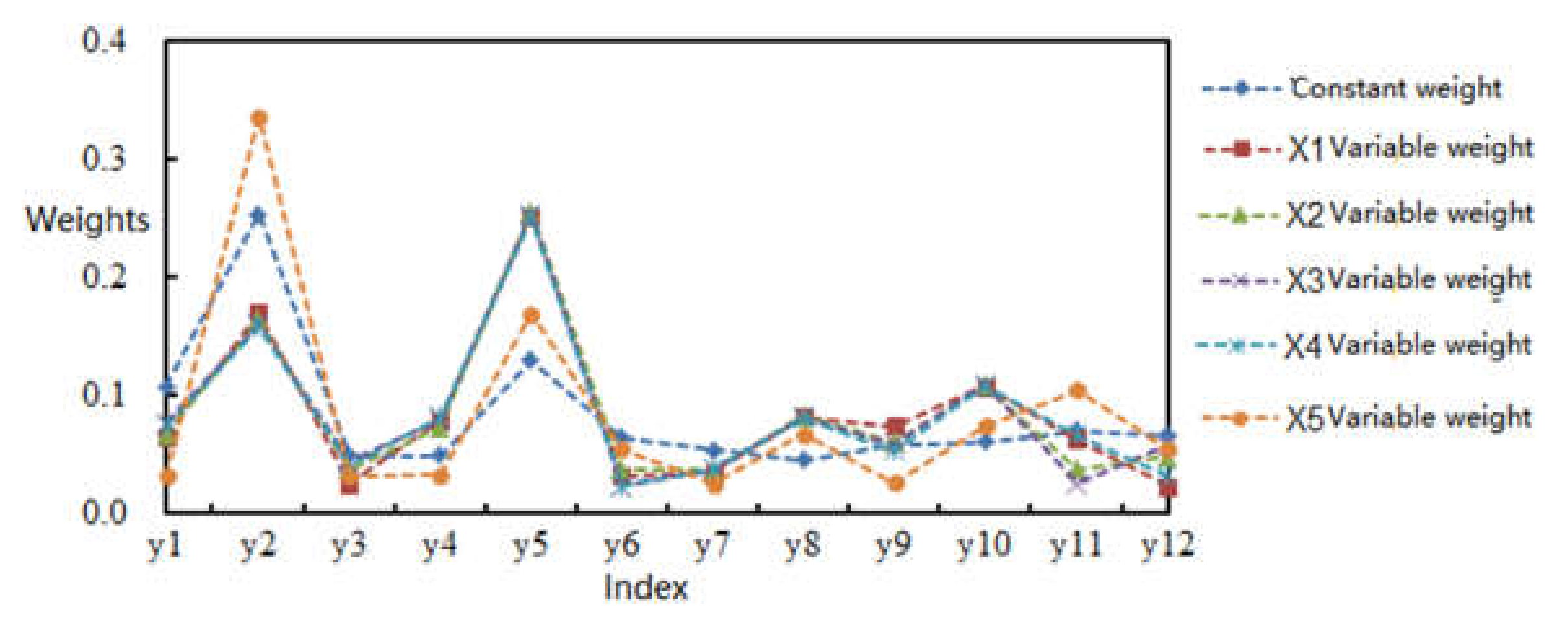
Combining the theory of extreme entropy weighting and variable weight, the constant weight of the slope rock mass stability evaluation index and the variable weight of rock mass to be evaluated are calculated using Equations (9)–(15) and (18), as shown in Table 4. As shown in Figure 4, the constant weight of the evaluation index reflects the relative importance of each evaluation index and the overall trend of the index weight. The influence of different index values on the weight is considered in the variable weight. Therefore, when the value of the same index is different, the weight will change. The variation law shows that when the index value is relatively good, the index weight will be greater; when the index value is relatively poor, the index weight will be smaller.
According to Equations (1)–(5), (16), and (17), the single index correlation of the slope rock mass sample with respect to each stability grade is calculated, as shown in Table 5. Similarly, the upper and lower limit index values of each grade in the classification evaluation index standard of the slope rock mass stability are calculated, as well as the single index correlation of the index values of the slope rock mass samples , , and with respect to each stability grade. Subsequently, the comprehensive correlation is calculated using Equation (6). Finally, the slope rock mass stability is calculated using Equations (7) and (8), and the upper and lower limits of each grade and the eigenvalues of the corresponding grade variables of the slope rock mass are also obtained, as is shown in Table 6 and Table 7. Based on Table 6, the corresponding stability grade of each slope rock mass sample can be determined according to the variable eigenvalue.
To prove the validity of the evaluation results, under the same evaluation index system, the evaluation results are obtained by using the hierarchical extension model, the multi-level unascertained measure-set pair analysis model, and the actual stability of the project, as shown in Table 7. A comparison of the results shows that the classification results of the slope rock mass obtained by the proposed model are consistent with the actual situation of the mine slope. Moreover, the evaluation results of the proposed model are more accurate than those of the hierarchical extension model and the multi-level unascertained measure-set pair analysis model.
6. Conclusions
- (1)
- The evaluation index dimension was unified using the extremum method, and the objective constant weight of the evaluation index (namely, uniaxial compressive strength; elastic modulus; Poisson’s ratio; structural features; cohesion force; internal friction; and daily maximum rainfall) was calculated using the entropy weight method. The constant weight reflects the relative importance of the evaluation indexes. On this basis, the variable weight theory was introduced to fully consider the influence of the value difference of the classification evaluation index on the index weight, and the excitation feature variable weight function was used to calculate the weighting of the evaluation index of each rock mass, so that the weighting of the evaluation index was more reasonable.
- (2)
- By applying the matter–element extension model and grade-variable method, the variable interval corresponding to the evaluation index standard of the stability grade of the slope rock mass and the variable value of the stability grade of each rock mass were calculated, and the stability grade of each rock mass was obtained. The evaluation results presented in this study are consistent with the engineering practice and are more accurate than those of the hierarchical extension model and the multi-level unascertained measure-set pair analysis model.
- (3)
- The variable value of the slope rock mass stability grade was obtained by the integrated information of comprehensive correlation between the evaluation index value of the slope rock mass stability and each stability grade. The accuracy of the extension model, in the classification of the slope rock mass stability, can be improved by the classification of the slope rock mass stability through the interval of the variable values of the grades corresponding to the evaluation index standard and the variable values for each slope rock mass stability grade.
Author Contributions
Conceptualization, S.Y.; methodology, S.Y.; data curation, Z.X. and K.S.; formal analysis, Z.X. and K.S.; validation, S.Y.; resources, S.Y. and Z.X.; writing—original draft preparation, Z.X.; writing—review and editing, Z.X.; project administration, S.Y. All authors have read and agreed to the published version of the manuscript.
Funding
This research was funded by the National Natural Science Foundation Project of China under Grant No. 72088101 and No. 51404305, and the Innovation Fund Project of Central South University under Grant No. 2021zzts0283.
Institutional Review Board Statement
Not applicable.
Informed Consent Statement
Not applicable.
Data Availability Statement
Data is contained within the article.
Acknowledgments
The authors would like to express their thanks to the National Natural Science Foundation and Innovation Fund Project of Central South University.
Conflicts of Interest
The authors declare no conflict of interest.
References
- Wang, S.H.; Li, X.H.; Yao, J.R.; Gong, F.Q.; Li, X.; Du, K.; Tao, M.; Huang, L.Q.; Du, S.L. Experimental investigation of rock breakage by a conical pick and its application to non-explosive mechanized mining in deep hard rock. Int. J. Rock Mech. Min. Sci. 2019, 122, 104063. [Google Scholar] [CrossRef]
- Wang, S.F.; Sun, L.C.; Li, X.B.; Wang, S.Y.; Du, K.; Li, X.; Feng, F. Experimental investigation of cuttability improvement for hard rock fragmentation using conical cutter. Int. J. Geomech. 2021, 21, 06020039. [Google Scholar] [CrossRef]
- Yang, T.H.; Zhang, F.C.; Yu, Q.L.; Cai, M.F.; Li, H.Z. Research situation of open-pit mining high and steep slope stability and its developing trend. Rock Soil Mech. 2011, 32, 1437–1452. [Google Scholar]
- Wang, S.F.; Tang, Y.; Li, X.B.; Du, K. Analyses and predictions of rock cuttabilities under different confining stresses and rock properties based on rock indentation tests by conical pick. Trans. Nonferrous Met. Soc. China 2021, 31, 1766–1783. [Google Scholar] [CrossRef]
- Wang, S.F.; Tang, Y.; Wang, S.Y. Influence of brittleness and confining stress on rock cuttability based on rock indentation tests. J. Cent. South Univ. 2021, 28, 2786–2800. [Google Scholar] [CrossRef]
- Shi, W.H.; Yang, T.H.; Wang, P.T.; Hu, G.J.; Xiao, P. Anisotropy analysis method for stability of open-pit slope rock mass and its application. Chin. J. Geotech. Eng. 2014, 36, 1924–1933. [Google Scholar]
- Zhao, H.J.; Ma, F.S.; Guo, J.; Wu, Z.Q.; Zhang, Y.L. The influence of open pit to underground mining on the stability of slope rock mass. J. Coal Mine 2011, 36, 1635–1641. [Google Scholar]
- Du, S.G.; Yong, R.; Chen, J.Q.; Chen, J.Q.; Xia, C.C.; Li, G.P.; Liu, W.L.; Liu, Y.M.; Liu, H. Graded analysis for slope stability assessment of large open-pit mines. Chin. J. Rock Mech. Eng. 2017, 36, 2601–2611. [Google Scholar]
- Bar, N.; Kostadinovski, M.; Tucker, M.; Byng, G.; Rachmatullah, R.; Maldonado, A.; Pötsch, M.; Gaich, A.; McQuillan, A.; Yacoub, T. Rapid and robust slope failure appraisal using aerial photogrammetry and 3D slope stability models. Int. J. Min. Sci. Technol. 2020, 30, 651–658. [Google Scholar] [CrossRef]
- Arikan, F.; Yoleri, F.; Sezer, S.; Caglan, D.; Biliyul, B. Geotechnical assessments of the stability of slopes at the Cakmakkaya and Damar open pit mines (Turkey): A case study. Environ. Earth Sci. 2010, 61, 741–755. [Google Scholar] [CrossRef]
- Wang, X.; Kang, Q.; Qin, J.; Zhang, Q.; Wang, S. Application of AHP-extenics model to safety evaluation of rock slope stability. J. Cent. South Univ. Sci. Technol. 2013, 44, 2455–2462. [Google Scholar]
- Zhang, X.; Zhou, S.W.; Lin, P.; Tan, Z.; Chen, Z.; Jiang, S. Slope stability evaluation based on entropy coefficient-set pair analysis. Chin. J. Rock Mech. Eng. 2018, 37, 3400–3410. [Google Scholar]
- Huang, D.; Shi, X.Z.; Qiu, X.Y.; Gou, Y. Stability gradation of rock slopes based on multilevel uncertainty measure-set pair analysis theory. J. Cent. South Univ. Sci. Technol. 2017, 48, 1057–1064. [Google Scholar]
- Liu, L.L.; Zhang, S.H.; Liu, L.M. Model and application of AHP and ideal point method based on stability gradation of rock slope. Chin. J. Cent. South Univ. Sci. Technol. 2014, 10, 3499–3504. [Google Scholar]
- Bar, N.; Barton, N. The Q-slope method for rock slope engineering. Rock Mech. Rock Eng. 2017, 50, 3307–3322. [Google Scholar] [CrossRef]
- Pastor, J.L.; Riquelme, A.J.; Tomás, R.; Cano, M. Clarification of the slope mass rating parameters assisted by SMRTool, an open-source software. Bull. Eng. Geol. Environ. 2019, 78, 6131–6142. [Google Scholar] [CrossRef] [Green Version]
- Cai, W. Introduction of Extenics. Syst. Eng. Theory Pract. 1998, 18, 76–84. [Google Scholar]
- Cai, W. Extension theory and its application. Chin. Sci. Bull. 1999, 44, 673–682. [Google Scholar] [CrossRef]
- Xu, H.J.; Zhao, B.F.; Zhou, Y.; Liu, S.X. Evaluation on water disaster from roof strata based on the entropy-weight and matter-element extension model. J. Min. Saf. Eng. 2018, 35, 112–117. [Google Scholar]
- Cai, W.; Yang, C.Y. Basic theory and methodology on extenics. Chin. Sci. Bull. 2013, 58, 1190–1199. [Google Scholar]
- Yang, C.Y.; Cai, W. Recent research progress in dependent functions in extension sets. J. Guangdong Univ. Technol. 2012, 29, 7–14. [Google Scholar]
- Shi, Z.P.; Shan, T.H.; Liu, W.F.; Zhang, X.P. Comprehensive evaluation of power network operation risk based on matter-element extensible model. Power Syst. Technol. 2015, 39, 3233–3239. [Google Scholar]
- Chen, S.Y. Theory and Model of Variable Fuzzy Sets and Its Application; Dalian University of Technology Press: Dalian, China, 2009. [Google Scholar]
- Li, Z.Y.; Rong, W.Y.; Chen, Z.D. Evaluation of railway luggage and parcel transportation safety based on variable fuzzy sets theory. China Saf. Sci. J. 2018, 28, 186–190. [Google Scholar]
- Hu, B.Q.; Zhang, X. Improvement and application of extension evaluation method. J. Wuhan Univ. 2003, 36, 79–84. [Google Scholar]
- Zhu, X.A.; Wei, G.D. Discussion on the good standard of dimensionless method in entropy method. Stat. Decis. 2015, 31, 12–15. [Google Scholar]
- Wang, W.; Luo, Z.Q.; Xiong, L.X.; Jia, N. Research of goaf stability evaluation based on improved matter-element extension model. J. Saf. Environ. 2015, 15, 21–25. [Google Scholar] [CrossRef]
- Tang, X.W.; Zhou, Z.F.; Shi, Y. The variable weighted functions of combined forecasting. Comput. Math. Appl. 2003, 45, 723–730. [Google Scholar] [CrossRef] [Green Version]
- Wang, P.Z.; Li, H.X. Fuzzy System Theory and Fuzzy Computer; Science Publishing Company of Beijing: Beijing, China, 1996. [Google Scholar]
- Li, D.Q.; Li, H.X. The properties and construction of state variable weight vectors. J. Beijing Norm. Univ. Nat. Sci. 2002, 38, 455–461. [Google Scholar]
- Atanassov, K.T. Operators over interval-valued intuitionistic fuzzy sets. Fuzzy Sets Syst. 1994, 64, 159–174. [Google Scholar] [CrossRef]
- Li, H.X. Factor spaces and mathematical frame of knowledge represention (VIII). Fuzzy Syst. Math. 1995, 9, 1–9. [Google Scholar]
- GB/T 50218-2014, Engineering Rock Mass Classification Standard. Available online: https://www.chinesestandard.net/PDF/BOOK.aspx/GBT50218-2014 (accessed on 10 August 2021).
- GB/T 50218-1994, Engineering Rock Mass Classification Standard. Available online: https://www.chinesestandard.net/PDF/BOOK.aspx/GB50218-1994 (accessed on 10 August 2021).
- GB 50487-2008, Code for Engineering Geological Investigation of Water Resources and Hydropower. Available online: https://www.chinesestandard.net/PDF/BOOK.aspx/GB50487-2008 (accessed on 10 August 2021).
- Kang, Z.Q.; Zhou, H.; Feng, X.T.; Yang, C.X. Evaluation of high rock slope quality based on theory of extenics. J. Northeast. Univ. Nat. Sci. 2007, 28, 1770–1774. [Google Scholar]
- Mo, G.L.; Zhang, W.G.; Liu, Y.J. Construction of Variable Spatial Weight and Analysis of Spatial Effect. J. Syst. Manag. 2018, 27, 219–229. [Google Scholar]
Figure 1.
Evaluation index system of the slope rock mass stability.

Figure 2.
Evaluation process of the variable weight matter–element extension model for the classification of the slope rock mass stability.
Figure 2.
Evaluation process of the variable weight matter–element extension model for the classification of the slope rock mass stability.

Figure 3.
Distribution of the evaluation index values for each slope rock mass.


Figure 4.
Comparison between the constant weights and variable weights of the evaluation index for each slope rock mass (the quantity of X is associated with the slope rock mass).
Figure 4.
Comparison between the constant weights and variable weights of the evaluation index for each slope rock mass (the quantity of X is associated with the slope rock mass).


Table 1.
Evaluation index classification criteria of the slope rock mass stability.
| Grade | y1/MPa | y2/GPa | y3 | y4/% | c y5/MPa | y6/(°) |
| Level I (extremely stable) | [150,200] | [33.0,60.0] | [0,0.20] | [90,100] | [2.10,8.00] | [60,90] |
| Level II (stable) | [125,150) | [20.0,33.0) | [0.20,0.25) | [75,90) | [1.50,2.10) | [50,60) |
| Level III (basically stable) | [90,125) | [6.0,20.0) | [0.25,0.30) | [50,75) | [0.70,1.50) | [39,50) |
| Level IV (unstable) | [40,90) | [1.3,6.0) | [0.30,0.35) | [30,50) | [0.20,0.70) | [27,39) |
| Level V (extremely unstable) | [10,40) | [0,1.3) | [0.35,0.50) | [0,30) | [0.05,0.20) | [0,27) |
| Grade | v y7/km·s−1 | y8/mm | y9/MPa | y10/L∙(min.10m)−1 | h y11/m | 1/k y12/(°) |
| Level I (extremely stable) | [5.0,7.5] | [0,20] | [0,2] | [0,25] | [0,30] | [0,10] |
| Level II (stable) | [4.0,5.0) | (20,40] | (2,8] | (25,50] | (30,45] | (10,20] |
| Level III (basically stable) | [2.5,4.0) | (40,60] | (8,14] | (50,100] | (45,60] | (20,40] |
| Level IV (unstable) | [2.0,2.5) | (60,100] | (14,20] | (100,125] | (60,80] | (40,60] |
| Level V (extremely unstable) | [0,2.0) | (100,150] | (20,25] | (125,150] | (80,100] | (60,80] |
Table 2.
Evaluation indexes of the slope rock mass stability.
| Rock | Measured Values of Geological Indexes | ||||||
y1/MPa | y2/GPa | y3 | y4/% | c y5/MPa | y6/° | v y7/km·s−1 | |
| X1 | 52.60 | 2.3 | 0.27 | 90 | 17.80 | 31.8 | 3.700 |
| X2 | 53.00 | 2.0 | 0.21 | 85 | 17.80 | 35.6 | 3.789 |
| X3 | 61.60 | 1.9 | 0.18 | 90 | 23.10 | 24.6 | 3.847 |
| X4 | 60.04 | 1.9 | 0.19 | 92 | 23.10 | 24.6 | 3.896 |
| X5 | 28.97 | 25.7 | 0.22 | 57 | 5.08 | 52.0 | 3.200 |
| Rock | Measured Values of Environmental Indexes | Measured Values of Engineering Indexes | |||||
y8/mm | y9/MPa | y10/L∙(min·10 m)−1 | h y11/m | 1/k y12/° | |||
| X1 | 6.06 | 6.18 | 10 | 48 | 60 | ||
| X2 | 6.06 | 8.73 | 10 | 67 | 44 | ||
| X3 | 6.06 | 9.05 | 9 | 76 | 38 | ||
| X4 | 6.06 | 10.18 | 9.5 | 45 | 54 | ||
| X5 | 12.00 | 15.32 | 35 | 12 | 36 | ||
Table 3.
Normalized values of the evaluation indexes for the slope rock mass stability.
| Rock Sample | y1 | y2 | y3 | y4 | y5 | y6 | y7 | y8 | y9 | y10 | y11 | y12 |
|---|---|---|---|---|---|---|---|---|---|---|---|---|
| X1 | 0.22 | 0.04 | 0.46 | 0.90 | 1.00 | 0.35 | 0.49 | 0.96 | 0.75 | 0.93 | 0.52 | 0.25 |
| X2 | 0.23 | 0.03 | 0.58 | 0.85 | 1.00 | 0.40 | 0.51 | 0.96 | 0.65 | 0.93 | 0.33 | 0.45 |
| X3 | 0.27 | 0.03 | 0.64 | 0.90 | 1.00 | 0.27 | 0.51 | 0.96 | 0.64 | 0.94 | 0.24 | 0.53 |
| X4 | 0.26 | 0.03 | 0.62 | 0.92 | 1.00 | 0.27 | 0.52 | 0.96 | 0.59 | 0.94 | 0.55 | 0.33 |
| X5 | 0.10 | 0.43 | 0.56 | 0.57 | 0.63 | 0.58 | 0.43 | 0.92 | 0.39 | 0.77 | 0.88 | 0.55 |
Table 4.
Evaluation index weights.
| Index | y1 | y2 | y3 | y4 | y5 | y6 | y7 | y8 | y9 | y10 | y11 | y12 | |
|---|---|---|---|---|---|---|---|---|---|---|---|---|---|
| Constant weight | 0.107 | 0.254 | 0.048 | 0.048 | 0.129 | 0.063 | 0.053 | 0.045 | 0.057 | 0.060 | 0.070 | 0.066 | |
| Weighted variable | X1 | 0.065 | 0.169 | 0.025 | 0.078 | 0.252 | 0.031 | 0.034 | 0.081 | 0.074 | 0.107 | 0.062 | 0.022 |
| X2 | 0.066 | 0.164 | 0.037 | 0.072 | 0.255 | 0.037 | 0.036 | 0.082 | 0.060 | 0.108 | 0.036 | 0.047 | |
| X3 | 0.076 | 0.160 | 0.044 | 0.079 | 0.253 | 0.022 | 0.036 | 0.081 | 0.058 | 0.109 | 0.025 | 0.057 | |
| X4 | 0.073 | 0.158 | 0.041 | 0.081 | 0.251 | 0.022 | 0.037 | 0.080 | 0.052 | 0.107 | 0.066 | 0.031 | |
| X5 | 0.031 | 0.336 | 0.031 | 0.032 | 0.168 | 0.054 | 0.024 | 0.067 | 0.025 | 0.073 | 0.104 | 0.054 | |
Table 5.
Single index correlation of the slope rock mass X1.
| Index | Single Index Correlation | |||||||||||
|---|---|---|---|---|---|---|---|---|---|---|---|---|
| y1 | y2 | y3 | y4 | y5 | y6 | y7 | y8 | y9 | y10 | y11 | y12 | |
| I | −0.696 | −0.931 | −0.233 | 0.000 | 1.000 | −0.470 | −0.260 | 1.040 | −0.403 | 1.067 | −0.273 | −0.714 |
| II | −0.630 | −0.886 | −0.080 | 0.000 | 0.000 | −0.364 | −0.075 | −0.699 | 0.420 | −0.599 | −0.059 | −0.667 |
| III | −0.468 | −0.620 | 0.095 | −0.600 | 0.000 | −0.185 | 0.088 | −0.850 | −0.228 | −0.799 | 0.067 | −0.500 |
| IV | 0.418 | 0.810 | −0.115 | −0.800 | 0.000 | 0.177 | −0.245 | −0.900 | −0.559 | −0.900 | −0.200 | 0.000 |
| V | −0.228 | −0.309 | −0.258 | −0.857 | 0.000 | −0.131 | −0.315 | −0.940 | −0.691 | −0.920 | −0.400 | 0.000 |
Table 6.
Grade variable intervals and the slope rock mass stability grades.
| Grade | I | II | III | IV | V |
|---|---|---|---|---|---|
| Level Variable k | [1.00, 1.86) | [1.86, 2.43) | [2.43, 3.58) | [3.58, 4.27) | [4.27, 5] |
Table 7.
Evaluation results of the slope rock mass stability.
| Sample | Comprehensive Correlation | Level Variable k | The Proposed Model | Hierarchical-Extension Model [5] | Multi-Level Unascertained Measure-Set Pair Analysis Model [7] | Actual Situation | ||||
|---|---|---|---|---|---|---|---|---|---|---|
| S(1) | S(2) | S(3) | S(4) | S(5) | ||||||
| X1 | 0.155 | −0.315 | −0.361 | −0.127 | −0.405 | 2.04 | Level II | Level II | Level III | Level II |
| X2 | 0.144 | −0.323 | −0.337 | −0.123 | −0.384 | 2.05 | Level II | Level I | Level II (near Level III) | Level II |
| X3 | 0.172 | −0.368 | −0.359 | −0.155 | −0.392 | 1.93 | Level II (near Level I) | Level II | Level III | Level II |
| X4 | 0.201 | −0.364 | −0.359 | −0.165 | −0.394 | 1.88 | Level II (near Level I) | Level I | Level II | Level II |
| X5 | 0.289 | −0.111 | −0.312 | −0.475 | −0.508 | 1.62 | Level I | Level I | Level II | Level I |
Publisher’s Note: MDPI stays neutral with regard to jurisdictional claims in published maps and institutional affiliations. |
© 2021 by the authors. Licensee MDPI, Basel, Switzerland. This article is an open access article distributed under the terms and conditions of the Creative Commons Attribution (CC BY) license (https://creativecommons.org/licenses/by/4.0/).
Share and Cite
MDPI and ACS Style
Yang, S.; Xu, Z.; Su, K. Variable Weight Matter–Element Extension Model for the Stability Classification of Slope Rock Mass. Mathematics 2021, 9, 2807. https://0-doi-org.brum.beds.ac.uk/10.3390/math9212807
AMA Style
Yang S, Xu Z, Su K. Variable Weight Matter–Element Extension Model for the Stability Classification of Slope Rock Mass. Mathematics. 2021; 9(21):2807. https://0-doi-org.brum.beds.ac.uk/10.3390/math9212807
Chicago/Turabian StyleYang, Shan, Zitong Xu, and Kaijun Su. 2021. "Variable Weight Matter–Element Extension Model for the Stability Classification of Slope Rock Mass" Mathematics 9, no. 21: 2807. https://0-doi-org.brum.beds.ac.uk/10.3390/math9212807
Note that from the first issue of 2016, this journal uses article numbers instead of page numbers. See further details here.