Evaluating the Performances of Biomarkers over a Restricted Domain of High Sensitivity

Abstract

The burgeoning advances in high-throughput technologies have posed a great challenge to the identification of novel biomarkers for diagnosing, by contemporary models and methods, through bioinformatics-driven analysis. Diagnostic performance metrics such as the partial area under the $ROC$ ($pAUC$) indexes exhibit limitations to analysing genomic data. Among other issues, the inability to differentiate between biomarkers whose $ROC$ curves cross each other with the same $pAUC$ value, the inappropriate expression of non-concave $ROC$ curves, and the lack of a convenient interpretation, restrict their use in practice. Here, we have proposed the fitted partial area index ($FpAUC$), which is computable through an algorithm valid for any $ROC$ curve shape, as an alternative performance summary for the evaluation of highly sensitive biomarkers. The proposed approach is based on fitter upper and lower bounds of the $pAUC$ in a high-sensitivity region. Through variance estimates, simulations, and case studies for diagnosing leukaemia, and ovarian and colon cancers, we have proven the usefulness of the proposed metric in terms of restoring the interpretation and improving diagnostic accuracy. It is robust and feasible even when the $ROC$ curve shows hooks, and solves performance ties between competitive biomarkers.

1. Introduction

Numerous medicinal sciences and life science issues dealing with data from high-throughput experiments are focused on the identification of key biomarkers, and the development of predictive models and medical prognosis systems. In the literature, two of the most intensively statistical approaches used for evaluating and comparing the overall binary diagnostic performance, both of single markers and scoring functions combining several tests, have been the receiver operating characteristic ($ROC$) curve and the area under this $ROC$ curve ($AUC$).

The main goal of a diagnostic (bio)marker or classifier is basically to discriminate instances with a condition of interest ($D=1$) from those without such a condition ($D=0$), such as the presence of a suspect disease from absence of it, a positive response to a targeted therapy from a negative one, transcriptional activity of a sequence from inactivity, and faulty modules in software systems from non-faulty ones. A continuous marker, X, can be dichotomised into positive and negative instances by choosing one of the marker scores c as a cut-off point, also named the decision threshold. On the basis of the true status (real diagnosis) of each instance being known, named the gold standard, the diagnostic accuracy of a marker is mainly measured by its specificity and sensitivity. The first metric, also named the true negative ratio ($TNR$), is the probability for a negative instance to be correctly diagnosed as negative. The other one, also called the true positive ratio ($TPR$), is the probability for a positive instance to be correctly diagnosed as positive. Notice that the false-positive ratio ($FPR$ or 1-specificity) and $TPR$ (or sensitivity) represent the probability of type-I error and the complementary probability of type-II error, respectively. In addition, both $FPR$ and $TPR$ are functions of such a threshold running over the entire range of possible biomarker scores, defined formally as $FPR\left(c\right)=P(X_0>c)$ and $TPR\left(c\right)=P(X_1>c)$, where $X_0=\left(X\right|D=0)$ and $X_1=(X>c|D=1)$. The accuracy of a classifier is thereby measured by these two probabilities estimated at each diagnostic threshold through the $ROC$ curve. This two-dimensional plot displays the pairs $\left(FPR\right(c),TPR(c\left)\right)$ for all the thresholds c, and can be written either as $(x,ROC(x\left)\right)$ with $ROC\left(x\right)=TPR\circ FP{R}^{-1}\left(x\right)$ for $x=FPR\left(c\right)\in [0,1]$, or analogously as $(RO{C}^{-1}\left(y\right),y)$ with $RO{C}^{-1}\left(y\right)=FPR\circ TP{R}^{-1}\left(y\right)$ for $y=TPR\left(c\right)\in [0,1]$. Graphically, it depicts the trade-offs available between both aspects of biomarker diagnostic performance across all the range of possible thresholds. An increase in the sensitivity comes at the expense of a decrease in the specificity and vice versa [1,2,3].

The $AUC$ is commonly used in many $ROC$-based analyses [4,5] as a single global index or summary metric for evaluating the overall discriminative ability of a predictive and prognostic test to correctly classify instances into one of the two mutually exclusive states of the condition of interest. The empirical $AUC$ is equivalent to the Mann–Whitney U statistic, and its value is commonly interpreted as the probability that an instance randomly drawn among the ones with the condition of interest shows a marker score higher than an instance randomly selected from those instances without it [6,7]. It is assumed that the $ROC$ curve of a perfect biomarker would have $AUC=1$; i.e., such a classifier discriminates instances perfectly as with condition of interest or without it. Meanwhile, a completely random classifier would have an $ROC$ curve lying on the diagonal line (named chance line), i.e., $AUC=0.5$. In this case, the discriminatory predictive ability of this diagnostic test is no better-than-chance (chance performance). Hence, $AUC$ varies from 0.5 to 1 for $ROC$ curves reporting better-than-chance performance. The $AUC$ has other convenient interpretations, such as the average sensitivity value for all values of specificity or the average specificity value for all values of sensitivity [2]. This overall evaluation metric does not depend on both the cut-off value and the prevalence of the cases, and thus is invariant under the case-control sampling [8].

Comprehensive surveys on the technical and statistical aspects of $ROC$ analysis can be found in [1,9,10], and more recently in [2,3,11,12,13,14,15,16,17].

Nevertheless, not all the regions of the $ROC$ curve are of interest and importance in many bioinformatics and screening medical applications [18,19,20,21], since low $FPR$ and high $TPR$ are biologically relevant or clinically acceptable. For instance, a high specificity (low $FPR$) range on the horizontal bandaxis would be demanded for the detection of a rare disease or cancer screening in which it is important to “rule in” a disease (e.g., a disease whose treatment implies major side effects), see [22]. On the other hand, a high sensitivity (high $TPR$) range on the vertical axis would be a priority when it is important to “rule out” a disease (e.g., a fatal disease if untreated) a range of relatively high $TPR$s would be chosen, i.e., high sensitivities [3,23]. Thus, $AUC$ may not be a meaningful $ROC$-based metric of diagnostic performance in a pre-specified confined range. In such situations, the partial area under the $ROC$ curve ($pAUC$) attracts more attention as diagnostic accuracy metric by summarising the portion of the $ROC$ curve over a pre-specified range [23,24,25,26], such as the rule-out (high sensitivity) or rule-in (high specificity) regions [27].

However, the $pAUC$ has been questioned for the lack of a convenient interpretation, since a biomarker describing locally better-than-chance performance might well yield $pAUC$ values close to 0, in contrast to the conventional $AUC$. In addition, the $pAUC$ has some limitations as a metric of predictive accuracy such as in the two classifier comparisons with equal $pAUC$ values derived from $ROC$ curves crossing over the same restricted range, which continues unsolved [28].

To address such shortcomings, some $pAUC$ indexes have been developed by different transformations. Thus, the standardised partial $AUC$ ($SpAUC$) index provided by McClish [24] is focused on a specificity range $(FP{R}_1,FP{R}_2)$. Upper and lower plausible bounds of the $pAUC$ are proposed to scale the possible values into the interval $(0.5,1)$, and be thereby interpreted appropriately as a measure of diagnostic performance, see also [2,3]. As the upper limit of the $pAUC$ for the $SpAUC$ index, it was considered the rectangle with high the unit and base $(FP{R}_2-FP{R}_1)$ corresponding to the $pAUC$ of a perfect classifier ($ROC\left(x\right)=1$, for all $x\in (0,1)$) restricted to the specificity range $(FP{R}_1,FP{R}_2)$. Whereas the lower one was established as the $pAUC$ between $FP{R}_1$ and $FP{R}_2$ for a completely non-informative biomarker ($FPR\left(c\right)=TPR\left(c\right)$, for all c) given by the area of the trapezoid $(FP{R}_1,0)$, $(FP{R}_2,0)$, $(FP{R}_2,FP{R}_2)$ and $(FP{R}_1,FP{R}_1)$. Furthermore, Ma et al. [5] derived two important properties which facilitate a suitable use of this summary index for proper $ROC$ curves, i.e., $ROC$ curves bounded below by the diagonal line, $ROC\left(x\right)\ge x$. Nevertheless, the $SpAUC$ index could still present some drawbacks that limit its widespread use, since the lower bound used in the $SpAUC$ is not well-defined for improper $ROC$ curves, i.e., $ROC$ curves crossing the diagonal line which are frequent in practice [29,30,31,32,33]. Moreover, the $SpAUC$ is not able to distinguish between two crossing $ROC$ curves with equal $pAUC$ values in the range of interest. Vivo et al. [26] have provided an alternative $pAUC$ index for any restricted specificity range named the tighter partial area index ($TpAUC$) index which overcomes such limitations of the $SpAUC$. Recently, the $TpAUC$ has been implemented in the R/Bioconductor package $ROCpAI$ [34], which also offers functions to estimate $pAUC$ and $SpAUC$, and their respective stabilities provided by their confidence intervals using bootstrap resampling.

On the other hand, in order to summarise meaningfully the diagnostic performance of a biomarker over a high sensitivity range in which “rule out” a disease is important, Jiang et al. [23] proposed a dual $pAUC$ index, conceptually similar to the $SpAUC$, within the true-positive band $(TPR0,1)$. This normalised partial area ($NpAUC$) index comes from dividing the $pAUC$ by $1-TP{R}_0$, i.e., the area of the rectangle above the pre-selected high sensitivity. The $NpAUC$ can be interpreted as the average value of specificity for all sensitivity values above $TP{R}_0$ [2,3,23] and is also valid for use in improper settings. Nevertheless, as the authors mentioned, the values of this $NpAUC$ index might be less than 0.5. Moreover, although this partial area index is a more meaningful summary of diagnostic performance in high sensitivity situations, it could still present some drawbacks for comparing two or more diagnostic performances over the same restricted interval of $TPR$ values, since two portions of $ROC$ curves may differ in their shape but enclose the same $pAUC$ value.

In this work, to tackle such issues, an alternative $pAUC$ index called the fitted partial area index ($FpAUC$) is proposed to summarise the discriminatory performances of highly sensitive markers satisfying the following characteristics: (a) to be equivalent to full $AUC$ when $TP{R}_0=0$ for informative biomarkers, (b) to have a suitable interpretation as a diagnostic performance metric, (c) to be applicable for any $ROC$ curve shape, and (d) to be capable of distinguishing between two or more crossing $ROC$ curves with the equal $pAUC$ values. To do that, new upper and lower bounds are derived for the $pAUC$ over the interval $(TP{R}_0,1)$ by adding an important characteristic of the $ROC$ curve and involving all the possible shapes. Through an algorithm, we provide a complete framework for the evaluation of highly sensitive markers in terms of discriminatory capacity by the proposed $FpAUC$, which does surpass the mentioned drawbacks of the $NpAUC$. Moreover, our algorithm was implemented in the R programming language [35]. The code of the $FpAUC$ function and the required internal functions for its computing are available in the Supplementary Materials.

The rest of this paper is organised as follows. In Section 2, we derive fitter bounds for the $pAUC$ above a pre-specified sensitivity threshold under flexible assumptions, which do not only assume concave shapes as proper $ROC$ curves; they also extend to any $ROC$ curve shape. From these bounds, the construction of the novel $FpAUC$ index as a more meaningful metric of the $pAUC$ is discussed and provided through a general algorithm to compute it for any $ROC$ curve covering all possible situations in practice. In Section 3, the variance of the $FpAUC$ estimator is derived under the assumption of a binormal $ROC$ model, and the performance of the estimate of the $FpAUC$ index is also assessed via the results of simulation studies to verify the appropriateness of the proposed index. Moreover, applications to genomic datasets involving leukaemia and ovarian and colon cancers are illustrated in Section 4. The paper is completed with a discussion in Section 5.

2. ROC Partial Area for Highly Sensitive Diagnostic Markers

In this section, lower and upper bounds involved in the standardisation of the $pAUC$ are derived. We show that the boundaries provided here are fitter than those given in [23]. In addition, the $pAUC$ transformed into the $FpAUC$ index can produce more reliable performance estimates for highly sensitive markers with any $ROC$ curve shapes, satisfying the characteristics listed in the introduction.

2.1. Fitter Boundaries

We firstly considered the $pAUC$ restricted to the interval $(TP{R}_0,1)\subseteq (0,1)$, which is defined as the area that lies above $TP{R}_0$ under an ROC curve, mathematically expressed as follows:

$$A_{TP{R}_0}={\int }_{TP{R}_0}^1\left(1-FPR\circ TP{R}^{-1}\left(y\right)\right)dy$$

(1)

where the $TP{R}_0$ is a pre-selected sensitivity threshold for a given diagnostic test, $y\in [TP{R}_0,1]$ represents the y-coordinate of an $ROC$ curve, $TP{R}^{-1}\left(y\right)$ is the decision threshold for the diagnostic classification, and $FPR\left(TP{R}^{-1}\left(y\right)\right)$ corresponds to its x-coordinate of such an $ROC$ curve. The $A_{TP{R}_0}$ is bounded by 0 and 1. It is null when the interval is reduced to a point, and becomes identical to the $AUC$ when the interval $(0,1)$ is considered.

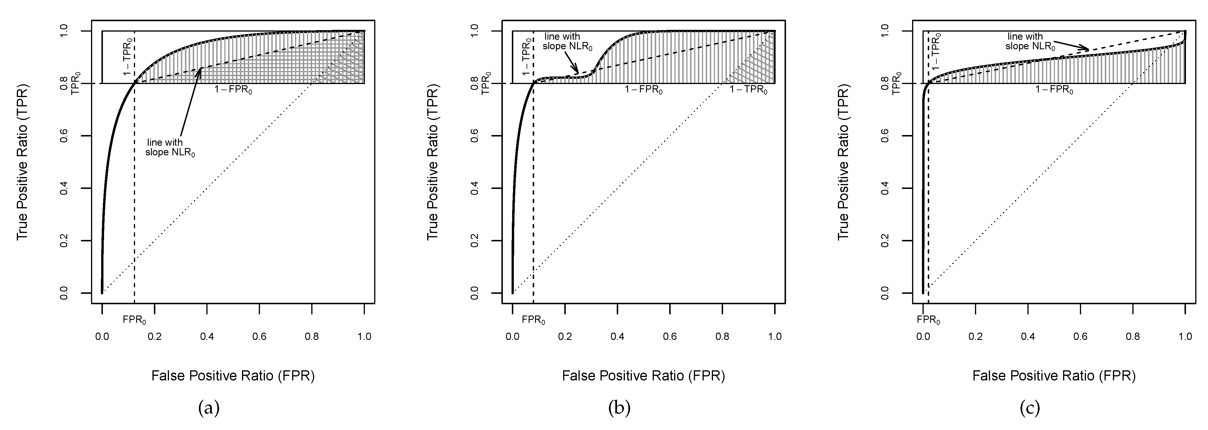
At first glance, $A_{TP{R}_0}$ is bounded above by the area of the rectangle of the $ROC$ space delimited by the band $(TP{R}_0,1)$ that encompasses it, i.e., the rectangle of side-lengths 1 and $1-TP{R}_0$. Moreover, when the ROC curve is proper in $(TP{R}_0,1)$, the $A_{TP{R}_0}$ is bounded below by the area of the triangle with corners ($TP{R}_0,TP{R}_0)$, $(1,TP{R}_0)$, and $(1,1)$ (see Figure 1a). Therefore, the following boundaries can be established:

$$\frac{1}{2}{(1-TP{R}_0)}^2\le A_{TP{R}_0}\le 1-TP{R}_0.$$

(2)

It is easily observed that this lower bound is only applicable for proper $ROC$ curves, which, on the other hand, implies that the $AUC$ is bounded by 0.5 and 1. In addition, notice that the upper bound in (2) was used by Jiang et al. [23] to scale the $A_{TP{R}_0}$, providing the $NpAUC$ index, which is a more meaningful and more accurate index in such a high-sensitivity region. This $NpAUC$ index will be further discussed in the next subsection.

Nevertheless, boundaries fitter than those given in (2) can be derived for the $A_{TP{R}_0}$. Thus, considering that an ROC curve is determined by the representation of pairs of $FPR$ and $TPR$, a fitter upper bound can be found by looking at the rectangle with apexes $(FP{R}_0,TP{R}_0)$ and $(1,1)$, where $FP{R}_0=FPR\left(TP{R}^{-1}\left(TP{R}_0\right)\right)$ (see Figure 1a). Thus, we have that the $A_{TP{R}_0}$ is closely bounded above by the area of the rectangle of height $1-TP{R}_0$ and width $1-FP{R}_0$; i.e.,

$$A_{TP{R}_0}\le (1-FP{R}_0)(1-TP{R}_0).$$

(3)

On the other hand, a narrower lower bound can be established to be also valid for any $ROC$ curve shape, by incorporating the negative likelihood ratio ($NLR$) of the $ROC$ curve of a classifier to the assumptions. The $NLR$ is defined as the false negative ratio $(1-TPR)$ over true negative ratio $(1-FPR)$, and can be mathematically expressed by $NLR\left(x\right)=(1-ROC(x\left)\right)/(1-x)$ for each point $(x,ROC(x\left)\right)$ on the $ROC$ curve. It provides a diagnostic performance metric of how many times patients with a disease are more (or less) likely to have a negative result than patients without the disease [36]. Furthermore, $NLR\left(x\right)$ represents the slope of the straight line which passes through the point of the $ROC$ curve and the upper-right corner $(1,1)$. For concave $ROC$ curves, the $NLR$ is monotone decreasing [5], and consequently, the portion of the curve in the horizontal band $(TP{R}_0,1)$ is above the straight line connecting $(FP{R}_0,TP{R}_0)$ and $(1,1)$ (see Figure 1a). By definition, the $ROC$ curve is monotonous non-decreasing, but it is not necessarily concave, since it might cross the chance line and/or display a hook showing locally worse-than-chance performance.

Hence, a lower boundary of the $A_{TP{R}_0}$ can be provided when the $NLR$ of the $ROC$ curve is bounded above by the lower extreme in the high sensitivity band $(TP{R}_0,1)$, i.e., $NLR\left(x\right)\le NL{R}_0$ for $x\ge FP{R}_0$ and $NL{R}_0=NLR\left(FP{R}_0\right)$, which will be called partially bounded $NLR$. Thereby, a fitter lower bound for the $A_{TP{R}_0}$ can be found by looking at the triangle with corners $(FP{R}_0,TP{R}_0)$, $(1,TP{R}_0)$, and $(1,1)$ (Figure 1a):

$$\frac{1}{2}(1-FP{R}_0)(1-TP{R}_0)\le A_{TP{R}_0}.$$

(4)

As is shown in Figure 1b, an $ROC$ curve can be partially proper in $(TP{R}_0,1)$. It is not concave over the entire high sensitivity range and dips below the line with slope $NL{R}_0$, but it does not cross the chance line, which becomes a lower limit of the $ROC$ curve in $(TP{R}_0,1)$. Thus, if there exists at least an $x\ge FP{R}_0$ such that $NLR\left(x\right)>NL{R}_0$, and $NLR\left(x\right)\le 1$ for all $x\ge FP{R}_0$, the $pAUC$ is bounded below by the area of triangle with vertices $(TP{R}_0,TP{R}_0)$, $(1,TP{R}_0)$, and $(1,1)$ (see Figure 1b):

$$\frac{1}{2}{(1-TP{R}_0)}^2\le A_{TP{R}_0}.$$

(5)

Finally, an $ROC$ curve might cross the chance line having a hook at the upper-right corner (see Figure 1c), which corresponds to grades of discriminatory accuracy worse than that of chance alone [37,38]. Thus, if there exists at least an $x\ge FP{R}_0$ such that $NLR\left(x\right)>max\{1,NL{R}_0\}$, then a positive lower bound of the $pAUC$ cannot be found:

$$0\le A_{TP{R}_0}.$$

(6)

Therefore, the $pAUC$ above a pre-selected sensitivity threshold $TP{R}_0$ of any diagnostic test can be classified in one of these three types based on the partial boundary of its $NLR$, providing fitter bounds to be used for building the $FpAUC$ index.

2.2. The Fitted Partial Area Index: $FpAUC$

In order to summarise the diagnostic performance in the horizontal band $(TP{R}_0,1)$, the $pAUC$ in (1) might be straight scaled by dividing it by the upper bound given in (2), which is the interval length of high sensitivity. Thereby, Jiang et al. [23] introduced the $NpAUC$ for highly sensitive diagnostic tests, which is mathematically expressed as follows:

$$A_{TP{R}_0}^{\prime }=\frac{A_{TP{R}_0}}{1-TP{R}_0}.$$

(7)

This normalisation satisfies the two first characteristics mentioned in the introduction. As is easy to see from (8), the $NpAUC$ becomes identical to the entire area when $TP{R}_0=0$. It may be interpreted as an average specificity value of the diagnostic marker over all values of $TPR$ between $TP{R}_0$ and 1 when such a marker is used to provide the high sensitivity range of practical interest. However, despite the fact that the value of the $NpAUC$ is bounded above by 1, its lower bound $(1-TP{R}_0)/2$ can have values of less than 0.5 for any classifier whose $pAUC$ is less than the half area of the horizontal band $(TP{R}_0,1)$. Furthermore, the $NpAUC$ index might still poorly compare diagnostic performances when two $ROC$ curves cross each other over the same high sensitivity range, inasmuch as two portions of $ROC$ curves may differ in shape but encompass the same $pAUC$ value, reporting the same $NpAUC$ value.

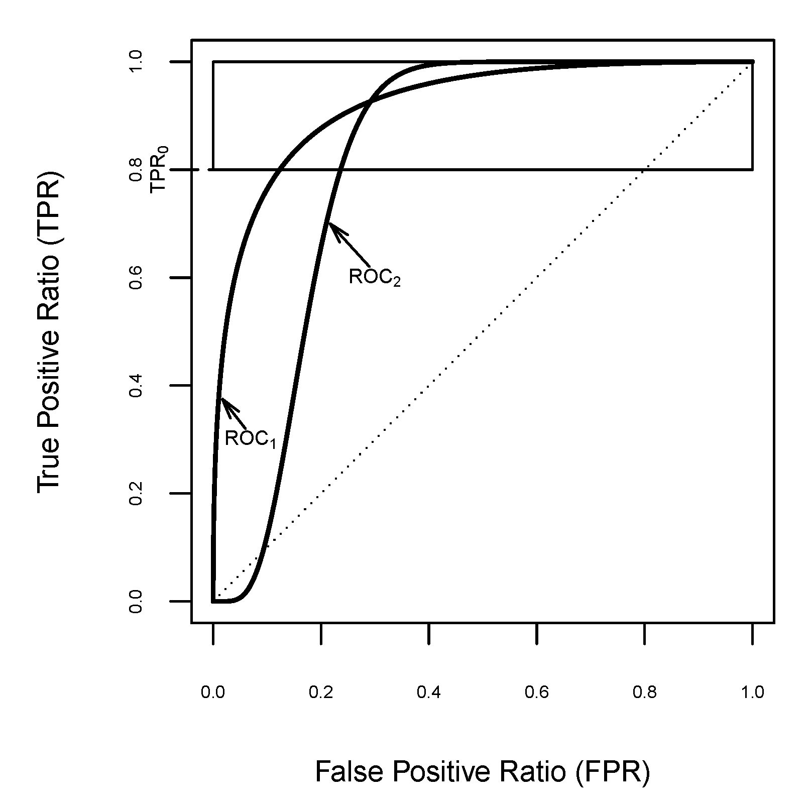
For illustrative purposes, let us suppose a clinical task demanding a high sensitivity, $TP{R}_0=0.8$, such as the discovery of new biomarkers for the detection of breast cancer in vast clinical samples. Amongst some diagnostic classifiers, there are two suitable candidates with the same performance for that sensitivity threshold, i.e., with the same $pAUC$ value, $A_{0.8}=0.142298$. Furthermore, their respective performances are described by the $ROC$ curves that cross the minimum sensitivity level at $FP{R}_0=0.1233548$ and $FP{R}_0=0.2362306$, respectively. Figure 2 displays these $ROC$ curves for highly sensitive diagnostic tests, from among others with the same $pAUC$ above the pre-selected sensitivity threshold $TP{R}_0=0.8$, which correspond to the conventional binormal model with the following binormal parameters: $a=2$ and $b=1$ for $RO{C}_1$; and $a=3.4070515591$ and $b=3.5706342338$ for $RO{C}_2$. The $NpAUC$ index provides the same value for both $ROC$ curves, $A_{0.8}^{\prime }=0.711491$. Thus, it is not appropriate for classifier comparison in such scenarios, since it is not sensitive for determining the best performance diagnostic test. Clearly, a new partial area index is necessary to assist in the identification of key biomarkers for biomedical decision making.

One alternative for measuring the discriminatory performance of the highly sensitive classifiers is to use a novel $pAUC$ index in the interval of practical interest. To do that, we propose the following transformation of the $A_{TP{R}_0}$:

$$A_{TP{R}_0}^{*}=\frac{1}{2}\left(1+\frac{A_{TP{R}_0}-min{A}_{TP{R}_0}}{max{A}_{TP{R}_0}-min{A}_{TP{R}_0}}\right)$$

(8)

where $min{A}_{TP{R}_0}$ and $max{A}_{TP{R}_0}$ are the fitter lower and upper bounds of $A_{TP{R}_0}$, respectively.

The $FpAUC$ index given by (8) reaches its minimum value of $1/2$ when $A_{TP{R}_0}^{*}=min{A}_{TP{R}_0}$, and its maximum value of 1 when $A_{TP{R}_0}^{*}=max{A}_{TP{R}_0}$. Furthermore, the characteristics mentioned in the introduction are satisfied, since it becomes identical to the entire area when $TP{R}_0=0$ for classifiers with better-than-chance performance, and can be interpreted as an average specificity value of a diagnostic test for all sensitivity values above $TP{R}_0$. In addition, the proposed $FpAUC$ index is mathematically well motivated and defined for any $ROC$ curve shape from their corresponding fitter bounds derived in Section 2.1. Hence, Algorithm 1 is provided to compute the $FpAUC$ value in the high sensitivity threshold $TP{R}_0$ according to the $ROC$ curve shape with respect to its $NLR$ over $(TP{R}_0,1)$.

Algorithm 1 Computing the $FpAUC$ value.

1: Set the high sensitivity threshold $TP{R}_0$. 2: $FP{R}_0=FPR\circ TP{R}^{-1}\left(TP{R}_0\right)$. 3: $NL{R}_0=(1-TP{R}_0)/(1-FP{R}_0)$. 4: $max{A}_{TP{R}_0}=(1-FP{R}_0)(1-TP{R}_0)$. 5: If $NLR\left(x\right)\le NL{R}_0$ for all $x\ge FP{R}_0$ then $min{A}_{TP{R}_0}=\frac{1}{2}(1-FP{R}_0)(1-TP{R}_0)$, and $$A_{TP{R}_0}^{*}=\frac{A_{TP{R}_0}}{(1-FP{R}_0)(1-TP{R}_0)}$$ (9) else if $NLR\left(x\right)\le 1$ for all $x\ge FP{R}_0$ then $min{A}_{TP{R}_0}=\frac{1}{2}{(1-TP{R}_0)}^2$, and $$A_{TP{R}_0}^{*}=\frac{A_{TP{R}_0}+(1-TP{R}_0)(TP{R}_0-FP{R}_0)}{(1+TP{R}_0-2FP{R}_0)(1-TP{R}_0)}$$ (10) else $$A_{TP{R}_0}^{*}=\frac{A_{TP{R}_0}+(1-TP{R}_0)(1-FP{R}_0)}{2(1-FP{R}_0)(1-TP{R}_0)}.$$ (11)

It is also worth remarking that the novel $FpAUC$ index involves both aspects of diagnostic performance represented in the restricted portion of an $ROC$ curve, $FPR$ and $TPR$.

Regarding the capacity of distinguishing between two or more classifiers, the $FpAUC$ index is more sensitive than the $NpAUC$. In practice, two $ROC$ curves might cross at a point where the sensitivity is higher than $TP{R}_0$, as shown in Figure 2, but they could encompass the same $pAUC$ in the horizontal band $(TP{R}_0,1)$. As in the above example, from the $NpAUC$ index, both curves cannot be compared above the pre-specified sensitivity threshold 0.8, but this can be done with the $FpAUC$ index because it always emphasises the performance differences for highly sensitive diagnostic tests.

In particular, for the above case study, the $pAUC$ transformed to $A_{0.8}^{*}$ reaches the value of 0.811606 for $RO{C}_1$, and the value is $A_{0.8}^{*}=0.931551$ for $RO{C}_2$. In other words, the proposed $FpAUC$ index allows us to unambiguously compare both diagnostic performances from the same sensitivity threshold. Thus, it might help with choosing the best tests for biomedical decision making, since the diagnostic test evaluated by the second $ROC$ curve has more relevance when a minimum sensitivity $TP{R}_0=0.8$ is clinically demanded; i.e., when its average specificity value is higher than the other in this region.

In Figure 2, it is clearly shown that $RO{C}_1$ has a higher $AUC$ value than $RO{C}_2$ does, namely, $AU{C}_{RO{C}_1}=0.921350$ and $AU{C}_{RO{C}_2}=0.820908$, which might drive one to discard the classifier $RO{C}_2$. However, the reported $FpAUC$ values revealed that the classifier $RO{C}_2$ performs much better than $RO{C}_1$ in the horizontal band $(0.8,1)$.

Similarly to [39] for $pAUC$, it was found that the $FpAUC$ as a metric is different from $AUC$, because a classifier with a higher value of $AUC$ does not necessarily lead to a higher value of $FpAUC$.

3. Performance of the Estimate of the $\mathit{FpAUC}$ Index

The performance of the $FpAUC$ index was assessed under the assumption of binormal $ROC$ models, by the variance of the $FpAUC$ estimator, and also through simulation studies in all plausible scenarios. The binormal model plays an important role in the signal detection theory for continuous classifiers [1], and is one of the most popular parametric models in $ROC$-based analyses, since it is obtained from the normality assumption of both groups, diseased or healthy subjects, or a monotone transformation of them [5,40]. In addition, the binormal $ROC$ model involves a wide variety of possible curve shapes, proper curves, and improper curves crossing the chance line either at the upper-right corner or at the lower-left corner, which enables us to describe the performance in different situations.

3.1. Variance of the $FpAUC$ Estimator

The variance of the $FpAUC$ estimator in the horizontal band $(TP{R}_0,1)$ can be obtained by using the first-order Taylor series approximation under the assumption of a parametric model, also known as the delta method (see among others [5,23,24,26]), or by using nonparametric resampling methods such as bootstrapping, an application of which to publicly available datasets is shown in the next section.

As aforementioned, the two-parametric binormal model is assumed to analyse the stochastic behaviour of the $FpAUC$ estimate and its variance. Concretely, the binormal model is derived from the assumption that the classifier scores are normally distributed in the group of healthy subjects, $X_0\sim N({\mu }_0,{\sigma }_0^2)$, and in the group of the disease subjects, $X_1\sim N({\mu }_1,{\sigma }_1^2)$. Thus, the $ROC$ curve for normally distributed test scores can be written as $ROC\left(x\right)=\Phi (a+b{\Phi }^{-1}\left(x\right))$, where $\Phi$ represents the standarised normal cumulative distribution function; $a=({\mu }_1-{\mu }_0)/{\sigma }_1$ and $b={\sigma }_0/{\sigma }_1$. Analogously, it can also be expressed by $RO{C}^{-1}\left(y\right)=\Phi \left(\left({\Phi }^{-1}\left(y\right)-a\right)/b\right)$. It is named the binormal $ROC$ curve, having parameters a and b, and without loss of generality, it can be assumed ${\mu }_0=0$, ${{\sigma }_0}^2=1$ and ${\mu }_1\ge 0$ due to the invariance of the $ROC$ curve under strictly increasing transformations of the classifier.

Under this theoretical framework, the $pAUC$ above a pre-specified sensitivity threshold $TP{R}_0$ given in (1) can be rewritten as

$$A_{TP{R}_0}={\int }_{TP{R}_0}^1\left(1-\Phi \left(\frac{{\Phi }^{-1}\left(y\right)-a}{b}\right)\right)dy={\int }_{{\Phi }^{-1}\left(TP{R}_0\right)}^{\infty }{\int }_{\frac{t-a}{b}}^{\infty }\varphi \left(x\right)\varphi \left(t\right)dxdt$$

where the last equality follows by substituting $t={\Phi }^{-1}\left(y\right)$. Moreover, taking into account the change $(t=-u,x=(\rho u-v){\left(1-{\rho }^2\right)}^{-1/2})$, the former equation can be expressed as

$$\begin{array}{cc}\hfill A_{TP{R}_0}& ={\int }_{-\infty }^{-{\Phi }^{-1}\left(TP{R}_0\right)}{\int }_{-\infty }^{\frac{a}{\sqrt{1+b^2}}}{\varphi }_B(u,v;\rho )dudv\hfill \\ \hfill & ={\Phi }_B\left(-{\Phi }^{-1}\left(TP{R}_0\right),\frac{a}{\sqrt{1+b^2}};\rho =\frac{-1}{\sqrt{1+b^2}}\right)\hfill \end{array}$$

(12)

where ${\varphi }_B$ and ${\Phi }_B$ are the density and cumulative distribution functions of the standard bivariate normal model with correlation coefficient $\rho$, respectively. An equivalent expression was used in [23].

Therefore, for an admissible minimum $TP{R}_0$, the partial area estimate ${\widehat{A}}_{TP{R}_0}$ can be computed through (12) using the maximum likelihood estimates of the binormal $ROC$ curve parameters, $\widehat{a}$ and $\widehat{b}$, as functions of the estimated mean and variance for the healthy and disease groups, respectively, $\widehat{a}=({\widehat{\mu }}_1-{\widehat{\mu }}_0)/{\widehat{\sigma }}_1$ and $\widehat{b}={\widehat{\sigma }}_0/{\widehat{\sigma }}_1$ (see among others [2,3]). Hence, the $FpAUC$ can be estimated from ${\widehat{A}}_{TP{R}_0}$ by using the expressions (9)–(11) given in Algorithm 1 according to the $ROC$ curve shape with respect to its $NLR$ in the horizontal band $(TP{R}_0,1)$.

For any high sensitivity range $(TP{R}_0,1)$, the variance of the $FpAUC$ estimate for the fitted binormal $ROC$ curve can be approximated by using the delta method as follows:

$$\widehat{Var}\left({\widehat{A}}_{TP{R}_0}^{*}\right)={\left(\frac{\partial {\widehat{A}}_{TP{R}_0}^{*}}{\partial a}\right)}^2\widehat{Var}\left(\widehat{a}\right)+{\left(\frac{\partial {\widehat{A}}_{TP{R}_0}^{*}}{\partial b}\right)}^2\widehat{Var}\left(\widehat{b}\right)+2\frac{\partial {\widehat{A}}_{TP{R}_0}^{*}}{\partial a}\frac{\partial {\widehat{A}}_{TP{R}_0}^{*}}{\partial b}\widehat{Cov}(\widehat{a},\widehat{b})$$

(13)

where

$$\widehat{Var}\left(\widehat{a}\right)=\frac{n_0(a^2+2)+2n_1{b}^2}{2n_0{n}_1},\widehat{Var}\left(\widehat{b}\right)=\frac{(n_0+n_1)b^2}{2n_0{n}_1},\widehat{Cov}(\widehat{a},\widehat{b})=\frac{ab}{2n_1},$$

and $n_0$ and $n_1$ are the sample sizes of the healthy and disease groups, respectively, (e.g., see [5]).

Therefore, the partial derivatives of the $FpAUC$ estimator with respect to a and b are required to compute the variance (13) in the three cases, (9)–(11), established by Algorithm 1, which are represented for some particular binormal $ROC$ models in Figure 3. To do that, we also need to calculate the partial derivatives of the $pAUC$ given in (12):

$$\frac{\partial A_{TP{R}_0}}{\partial a}=h_0(a,b),\mathrm{and}\frac{\partial A_{TP{R}_0}}{\partial b}=-\frac{ab}{1+b^2}{h}_0(a,b),$$

where

$$h_0(a,b)=\frac{1}{\sqrt{1+b^2}}\varphi \left(\frac{a}{\sqrt{1+b^2}}\right)\Phi \left(\frac{\sqrt{1+b^2}}{b}\left(\frac{a}{1+b^2}-{\Phi }^{-1}\left(TP{R}_0\right)\right)\right).$$

In the first case, when the binormal $ROC$ curve has partially bounded $NLR$ in the horizontal band $(TP{R}_0,1)$, i.e., $NLR\left(x\right)\le NLR\left(FP{R}_0\right)$ for all $x\ge FP{R}_0$, the $FpAUC$ estimator can be written in terms of the parameters a and b, by substituting (12) into (9), as

$$A_{TP{R}_0}^{*}=\frac{{\Phi }_B\left(-{\Phi }^{-1}\left(TP{R}_0\right),\frac{a}{\sqrt{1+b^2}};\rho =\frac{-1}{\sqrt{1+b^2}}\right)}{(1-TP{R}_0)\left(1-\Phi \left(-g_0(a,b)\right)\right)},$$

(14)

where $g_0(a,b)=\frac{a-{\Phi }^{-1}\left(TP{R}_0\right)}{b}$, and hence, its partial derivatives can be expressed as

$$\begin{array}{cc}\hfill \frac{\partial A_{TP{R}_0}^{*}}{\partial a}& =\frac{h_0(a,b)}{(1-TP{R}_0)\Phi \left(g_0(a,b)\right)}-\frac{\varphi \left(g_0(a,b)\right)A_{TP{R}_0}^{*}}{b\Phi \left(g_0(a,b)\right)}\hfill \\ \hfill \frac{\partial A_{TP{R}_0}^{*}}{\partial b}& =-\frac{ab{h}_0(a,b)}{(1+b^2)(1-TP{R}_0)\Phi \left(g_0(a,b)\right)}+\frac{g_0(a,b)\varphi \left(g_0(a,b)\right)A_{TP{R}_0}^{*}}{b\Phi \left(g_0(a,b)\right)},\hfill \end{array}$$

which enable us to compute the variance (13).

In the second case, the binormal $ROC$ curve does not have a partially bounded $NLR$, but it is above the chance line, i.e., $NLR\left(x\right)\le 1$ for all $x\ge FP{R}_0$, and there exists at least an $x^{\prime }>FP{R}_0$ such that $NLR\left(x^{\prime }\right)>NL{R}_0$. Here, the $FpAUC$ estimator can be written in terms of a and b parameters by substituting (12) into (10), as

$$A_{TP{R}_0}^{*}=\frac{{\Phi }_B\left({\Phi }^{-1}\left(TP{R}_0\right),\frac{a}{\sqrt{1+b^2}};\rho =\frac{-1}{\sqrt{1+b^2}}\right)+(1-TP{R}_0)\left(TP{R}_0-\Phi \left(-g_0(a,b)\right)\right)}{(1-TP{R}_0)\left(1+TP{R}_0-2\Phi \left(-g_0(a,b)\right)\right)},$$

(15)

whose partial derivatives with respect to the parameters a and b can be written as

$$\begin{array}{cc}\hfill \frac{\partial A_{TP{R}_0}^{*}}{\partial a}& =\frac{h_0(a,b)+\frac{(1-TP{R}_0)\varphi \left(g_0(a,b)\right)}{b}}{1-TP{R}_0^2-2(1-TP{R}_0)\Phi \left(-g_0(a,b)\right)}+\frac{2\varphi \left(g_0(a,b)\right)A_{TP{R}_0}^{*}}{b\left(1+TP{R}_0-2\Phi \left(-g_0(a,b)\right)\right)}\hfill \\ \hfill \frac{\partial A_{TP{R}_0}^{*}}{\partial b}& =-\frac{\frac{ab{h}_0(a,b)}{(1+b^2)}-\frac{(1-TP{R}_0)g_0(a,b)\varphi \left(g_0(a,b)\right)}{b}}{1-TP{R}_0^2-2(1-TP{R}_0)\Phi \left(-g_0(a,b)\right)}+\frac{2g_0(a,b)\varphi \left(g_0(a,b)\right)A_{TP{R}_0}^{*}}{b\left(1+TP{R}_0-2\Phi \left(-g_0(a,b)\right)\right)}.\hfill \end{array}$$

Finally, in the third case, the $NLR$ of the binormal $ROC$ curve cannot be upper bounded in the horizontal band $(TP{R}_0,1)$, and thus, by substituting (12) into (11), the $FpAUC$ estimator can be written in terms of a and b as

$$A_{TP{R}_0}^{*}=\frac{{\Phi }_B\left({\Phi }^{-1}\left(TP{R}_0\right),\frac{a}{\sqrt{1+b^2}};\rho =\frac{-1}{\sqrt{1+b^2}}\right)+(1-TP{R}_0)\Phi \left(g_0(a,b)\right)}{2(1-TP{R}_0)\Phi \left(g_0(a,b)\right)},$$

(16)

and then, its variance can be computed from (13) by using the following partial derivatives with respect to the parameters a and b:

$$\begin{array}{cc}\hfill \frac{\partial A_{TP{R}_0}^{*}}{\partial a}& =\frac{h_0(a,b)+\frac{(1-TP{R}_0)\varphi \left(g_0(a,b)\right)}{b}}{2(1-TP{R}_0)\Phi \left(g_0(a,b)\right)}-\frac{\varphi \left(g_0(a,b)\right)A_{TP{R}_0}^{*}}{b\Phi \left(g_0(a,b)\right)}\hfill \\ \hfill \frac{\partial A_{TP{R}_0}^{*}}{\partial b}& =-\frac{\frac{ab{h}_0(a,b)}{(1+b^2)}+\frac{(1-TP{R}_0)g_0(a,b)\varphi \left(g_0(a,b)\right)}{b}}{2(1-TP{R}_0)\Phi \left(g_0(a,b)\right)}-\frac{g_0(a,b)\varphi \left(g_0(a,b)\right)A_{TP{R}_0}^{*}}{b\Phi \left(g_0(a,b)\right)}.\hfill \end{array}$$

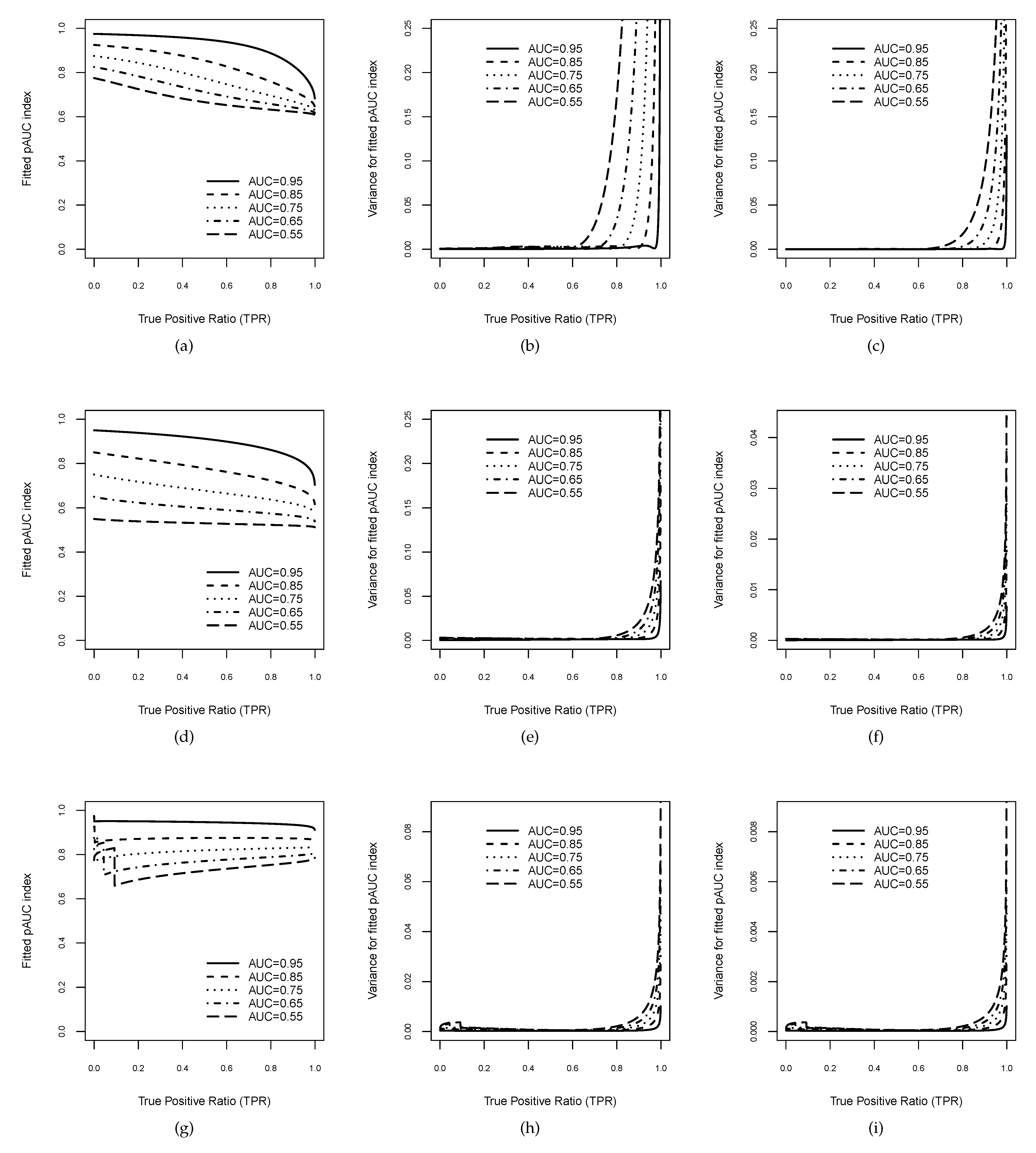
In order to illustrate the stochastic behaviour of the $FpAUC$ estimate and its variance, Figure 3 displays examples of binormal $ROC$ models, including each one of possible curve shapes: concave $ROC$ curves for $b=1$ (Figure 3d–f), improper $ROC$ curves crossing the chance line in the upper-right corner for $b=0.5<1$ (Figure 3a–c), and improper $ROC$ curves crossing the chance line in the lower-left corner for $b=2>1$ (Figure 3g–i).

For each value of b, five binormal $ROC$ curves with $AUC$ values of $0.55$, $0.65$, $0.75$, $0.85$, and $0.95$ were considered, and consequently, the parameter $a=\sqrt{1+b^2}{\Phi }^{-1}\left(AUC\right)$ was derived from the values of b and $AUC$, since $AUC=\Phi \left(\frac{a}{\sqrt{1+b^2}}\right)$ [10]. The three graphics on the left column (Figure 3a,d,g) depict the behaviour of the $FpAUC$ estimates (14)–(16) as a function of high sensitivity threshold $TP{R}_0$. As is shown in Figure 3g for $b>1$, the binormal $ROC$ curves have a hook at the beginning, causing a change in the boundary of the $NLR$ above $TP{R}_0$, whereas this is not the case for $b\le 1$. The remaining six graphics on the central and right columns display the behaviour of the variances of the $FpAUC$ as functions of $TP{R}_0$. Obviously, (13) depends on the sample sizes assumed for the healthy and disease groups, $n_0$ and $n_1$, respectively. Thus, we have considered two different settings. The central column shows Figure 3b,e,h for $n_0=n_1=50$, and the right column corresponds to Figure 3c,f,i for $n_0=n_1=500$. In general, all variance estimates suggest relatively good accuracy by the $FpAUC$ index, since they are very small and tend to 0 as the high sensitivity range increases. In particular, this behaviour is also shown for $b>1$ in Figure 3h,i, although the hook at the beginning produced a discontinuity point due to the change of the $NLR$ boundary.

3.2. Simulation Studies

Through a set of simulation studies, the performance of the $FpAUC$ estimates was assessed in terms of biases, standard deviations, and percentile confidence intervals (CI), proving the operating properties of the proposed $FpAUC$ index, such as its robustness and feasibility, even when the fitted $ROC$ curve has hooks and/or crosses the chance line over a high sensitivity range.

Similarly to the simulation studies in [5,26], test scores both for healthy ($X_0$) and diseased ($X_1$) subjects were generated from normal distributions with parameters set appropriately to obtain binormal $ROC$ curves: $AUC=0.55$, $0.65$, $0.75$, $0.85$, and $0.95$; and $b=0.5$, 1, 2, and 3. Such settings for parameter b allowed us to analyse the different shapes of the underlying binormal $ROC$ curve, concave $ROC$ curves ($b=1$), and improper $ROC$ curves ($b\ne 1$), including curves crossing the chance line with a hook at the upper-right corner ($b<1$) and with a hook at the lower-left corner ($b>1$).

In all scenarios, $\mathrm{10,000}$ random samples were generated with sample sizes equal to 100 ($n_0=n_1=50$) and 1000 ($n_0=n_1=500$), as the ones taken in [23]. Without loss of generality, the $n_0$ healthy subjects were drawn from $N\left({\mu }_0=0,{\sigma }_0^2=1\right)$ and the $n_1$ diseased ones from $N\left({\mu }_1=a/b,{\sigma }_1^2=1/b^2\right)$, and as aforementioned, the separation coefficient $a=\sqrt{1+b^2}{\Phi }^{-1}\left(AUC\right)$ was derived from the values of b and $AUC$ of the binormal $ROC$ curve.

Within each one of the simulation scenarios, empirical means and standard deviations were computed from the $\mathrm{10,000}$ estimations of the $FpAUC$ index, for five high sensitivity thresholds $TP{R}_0=0.9$, $0.8$, $0.7$, $0.6$, and $0.5$. Biases of the $FpAUC$ estimates are also reported. Furthermore, the percentile method was applied to construct the $95\%$ CI for the $FpAUC$ value, by taking the $2.5\%$ trimmed ranges of each $\mathrm{10,000}$ estimations.

For the sake of brevity,

Table 1. Simulation results from $\mathrm{10,000}$ random samples with size $n=100$ for each binormal $ROC$ model. The first two columns correspond to the settings of each scenario, which were used to compute the $FpAUC$ estimates for each $TP{R}_0$, and to summarise its mean, bias, standard deviation, and $95\%$ CI.

b	$\mathit{AUC}$	${\mathit{TPR}}_0$	$\mathit{FpAUC}$			$95\%$ CI
			Mean	Bias	SD	Low	Up
0.5	0.75	0.9	0.6718115	0.002067363	0.03374133	0.6109004	0.7431961
		0.8	0.6973917	0.002155138	0.03558272	0.6320246	0.7713159
		0.7	0.7228261	0.002184195	0.03660373	0.6538301	0.7981706
		0.6	0.7488924	0.002003218	0.0369359	0.678575	0.8235492
		0.5	0.7750897	0.001550933	0.03635573	0.7046808	0.8474584
	0.85	0.9	0.7168091	−0.0001375311	0.03876775	0.64157	0.7885817
		0.8	0.757652	−0.0009985873	0.03997576	0.6777845	0.8318443
		0.7	0.7934277	−0.001905229	0.03933383	0.7136111	0.8671967
		0.6	0.8244922	−0.002902352	0.03702263	0.7476242	0.8926417
		0.5	0.8506002	−0.003705619	0.03402315	0.7800026	0.9118017
	0.95	0.9	0.8047574	−0.02685653	0.0437217	0.7093416	0.8801134
		0.8	0.860915	−0.02640532	0.03803334	0.774634	0.9257051
		0.7	0.8952863	−0.02358188	0.03181761	0.8217905	0.9472467
		0.6	0.9171706	−0.02071222	0.02667352	0.8543599	0.9597633
		0.5	0.9319396	−0.01811886	0.02250016	0.8789607	0.9674647
1	0.75	0.9	0.6419233	0.02250682	0.05648455	0.547629	0.7509011
		0.8	0.6561746	0.01883174	0.05412381	0.5630157	0.7638427
		0.7	0.6681171	0.016265	0.05257736	0.5753191	0.7748332
		0.6	0.6795033	0.01444329	0.05158024	0.5865734	0.7865055
		0.5	0.6907137	0.01294236	0.051032	0.5972964	0.7980257
	0.85	0.9	0.6990107	0.003745407	0.05494855	0.5908895	0.8023507
		0.8	0.7254672	0.00285371	0.05170491	0.6216724	0.82305
		0.7	0.7461418	0.002565651	0.04913346	0.6469846	0.8389251
		0.6	0.7640257	0.00239235	0.04698019	0.6694555	0.8530543
		0.5	0.7801295	0.002110163	0.04530041	0.6880103	0.8665002
	0.95	0.9	0.8270716	−0.0007875378	0.04783165	0.7247062	0.9113977
		0.8	0.8604097	−0.0005883846	0.04115932	0.7717688	0.9325321
		0.7	0.8820235	−0.0006256009	0.03651525	0.8028981	0.945313
		0.6	0.8980373	−0.0007762952	0.03285448	0.8263655	0.9547746
		0.5	0.9106385	−0.0009819187	0.02980191	0.8449012	0.9616409
2	0.75	0.9	0.8284354	−0.001861235	0.03295873	0.7575531	0.885924
		0.8	0.8265318	−0.001388059	0.0321334	0.7576136	0.8829055
		0.7	0.8243309	−0.001014902	0.03170301	0.7564865	0.8805151
		0.6	0.821783	−0.0006798947	0.03150106	0.754266	0.8783047
		0.5	0.8187734	−0.0003587272	0.03149208	0.7520585	0.8759183
	0.85	0.9	0.8720737	−0.001061615	0.02696685	0.8130079	0.9186131
		0.8	0.8741264	−0.000593173	0.02599251	0.8179064	0.9201215
		0.7	0.8750833	−0.0002584535	0.02553713	0.8201296	0.9207303
		0.6	0.875456	0.00001478198	0.02536532	0.8213299	0.9211979
		0.5	0.875372	0.0002512013	0.02541599	0.8213275	0.9216513
	0.95	0.9	0.9346536	−0.0002348478	0.01772344	0.895961	0.9654708
		0.8	0.9396177	−0.0000273009	0.01681173	0.9031781	0.9692494
		0.7	0.9427292	0.00006276168	0.0163881	0.907249	0.9717697
		0.6	0.9450175	0.00009651483	0.01618441	0.9102256	0.9738309
		0.5	0.9468161	0.00009179076	0.01612146	0.9120827	0.9755344

displays the results corresponding to $AUC$ values equal to $0.75$, $0.85$ and $0.95$ and b values equal to $0.5$, 1, and 2, which were obtained from the simulation study for $n=100$. The simulation results for $n=1000$ can be found in Appendix A 

Table A1. Simulation results from $\mathrm{10,000}$ random samples with size $n=1000$ for each binormal $ROC$ model.

b	$\mathit{AUC}$	${\mathit{TPR}}_0$	$\mathit{FpAUC}$			$95\%$ CI
			Mean	Bias	SD	Low	Up
0.5	0.75	0.9	0.669964	0.0002198603	0.0108208	0.64931	0.6914392
		0.8	0.6954584	0.0002217709	0.01145733	0.6734022	0.7183308
		0.7	0.7208582	0.0002162642	0.01182557	0.6981509	0.7442612
		0.6	0.7470829	0.0001937058	0.01195146	0.7239764	0.7708441
		0.5	0.7736821	0.0001433617	0.01178972	0.7508544	0.7972385
	0.85	0.9	0.7172018	0.000255154	0.01312834	0.6920607	0.743343
		0.8	0.7588624	0.0002117937	0.01361137	0.7323675	0.785571
		0.7	0.7954699	0.0001369812	0.0133132	0.7694111	0.821656
		0.6	0.8274379	0.00004334917	0.01244126	0.8028483	0.8519594
		0.5	0.8542618	−0.0000439935	0.01121478	0.8320698	0.8760613
	0.95	0.9	0.8262998	−0.005314134	0.01523457	0.7971094	0.8518365
		0.8	0.8783896	−0.008930742	0.01638089	0.8212213	0.8990199
		0.7	0.9072943	−0.01157388	0.01663234	0.8560455	0.9263972
		0.6	0.9250275	−0.01285529	0.01586612	0.8823802	0.9437126
		0.5	0.9367677	−0.01329082	0.01478211	0.901801	0.9548009
1	0.75	0.9	0.6192974	−0.0001190819	0.01974289	0.5798105	0.6567464
		0.8	0.6372461	−0.00009677	0.01869301	0.5999832	0.6730179
		0.7	0.6517819	−0.0000701156	0.01786319	0.6159922	0.6862381
		0.6	0.6650315	−0.0000285186	0.01716452	0.6306253	0.6981055
		0.5	0.6777806	0.000 0924348	0.01657033	0.644864	0.7097416
	0.85	0.9	0.695105	−0.0001602661	0.01877502	0.6576742	0.730797
		0.8	0.7225075	−0.0001059672	0.01737564	0.6875739	0.7555136
		0.7	0.7435126	−0.0000635848	0.01633348	0.7103603	0.7747373
		0.6	0.7615994	−0.000033939	0.01549253	0.7301897	0.7913494
		0.5	0.7780006	−0.0000187107	0.01478812	0.7481515	0.8063218
	0.95	0.9	0.8276785	−0.0001805795	0.01527662	0.7964039	0.8564896
		0.8	0.8608451	−0.0001529308	0.01316279	0.8338855	0.8856906
		0.7	0.8824989	−0.0001502163	0.01170487	0.8588247	0.9045469
		0.6	0.8986535	−0.0001600285	0.01055402	0.8772063	0.918292
		0.5	0.9114447	−0.0001757661	0.009580882	0.8920362	0.9290016
2	0.75	0.9	0.8300773	−0.0002192794	0.01031469	0.8090532	0.8494656
		0.8	0.8277414	−0.0001785075	0.01008743	0.8071688	0.8468292
		0.7	0.8251995	−0.0001463208	0.009972896	0.8048588	0.8440616
		0.6	0.8223455	−0.0001174049	0.009923987	0.8022668	0.8412388
		0.5	0.8190425	−0.0000896712	0.009931295	0.798934	0.8380641
	0.85	0.9	0.8729891	−0.0001461737	0.008438532	0.8558683	0.8888247
		0.8	0.8746149	−0.0001046822	0.008160062	0.8577607	0.8900416
		0.7	0.8752668	−0.0000749573	0.008033339	0.8585469	0.8905781
		0.6	0.8753906	−0.0000506706	0.007990856	0.8588198	0.8906265
		0.5	0.8750911	−0.0000296841	0.00801607	0.8585946	0.8903774
	0.95	0.9	0.9348269	−0.0000615823	0.005566497	0.9233001	0.945249
		0.8	0.9396036	−0.0000413422	0.00530871	0.9287226	0.9495554
		0.7	0.9426341	−0.0000323708	0.005195553	0.93215	0.9522928
		0.6	0.944892	−0.0000289385	0.00514828	0.9344389	0.9544434
		0.5	0.9466949	−0.0000294023	0.005143699	0.9361809	0.9562475

. Full tables are available in the Supplementary Materials.

For both sample sizes, $n=100$ and $n=1000$, simulation results displayed in Table 1 and Table A1 agree with the ones depicted in Figure 3. For all the $\mathrm{10,000}$ simulated random samples in each setting, the $FpAUC$ index was always applicable, including the scenarios in which the fitted $ROC$ curves had hooks and crossed the chance line. In general, the stochastic behaviour of the $FpAUC$ estimates over each high sensitivity range was similar for both sample sizes. The biases of the $FpAUC$ estimates remained relatively stable and smaller than standard deviations. For the fitted $ROC$ curves with high global accuracy ($AUC\ge 0.85$), standard deviations and widths of the $95\%$ CIs tended to decrease as the sensitivity threshold decreased; i.e., the precision of the $FpAUC$ index increased as the high sensitivity range increased. However, for fitted curves with poor global accuracy ($AUC\le 0.65$), standard deviations and widths of the $95\%$ CIs slightly increased as the sensitivity range increased, although remaining relatively small; i.e., the precision of the $FpAUC$ index smoothly decreased as the sensitivity threshold decreased. In summary, the simulation studies showed reliable behaviour from the $FpAUC$ index, making it a relatively accurate metric with which to evaluate diagnostic performance over a high sensitivity interval.

4. Applications to Genomic Data

To further examine the performance of the proposed $FpAUC$ index for highly sensitive diagnostic tests, we analysed three experimental genomic datasets that are publicly available.

Before listing the results obtained, brief descriptions of the high-dimensional datasets are given next.

4.1. Ovarian Cancer Data

This dataset is concerned with the search for biomarkers of ovarian cancer in population screening [41], available at http://research.fhcrc.org/diagnostic-biomarkers-center, accesssed on 20 February 2021. Basically, it consists of mRNA expression, using glass array spotted for 1536 gene clones on 53 ovarian tissue samples, 23 healthy controls, and 30 cases with ovarian cancer.

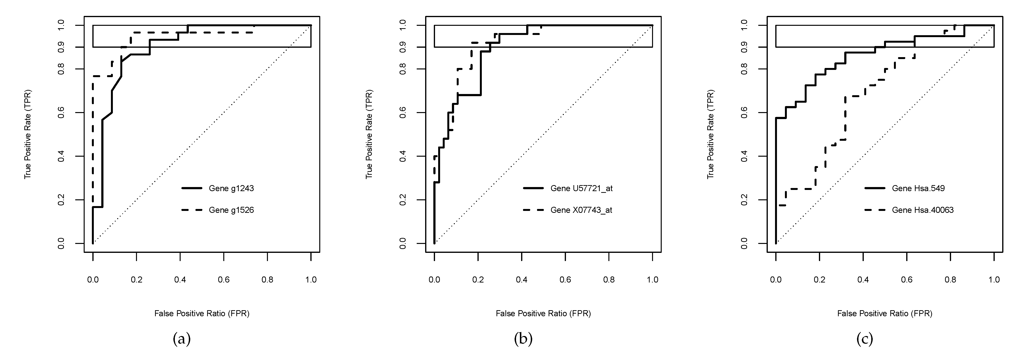
In this whole dataset, 1330 ($86.59\%$) out of the 1536 empirical $ROC$ curves resulted in being improper, and 136 ($8.85\%$) had $AUC\ge 0.8$. Moreover, 23 ($16.91\%$) out of such 136 curves crossed the chance line. In addition, $\mathrm{21,315}$ ($2.72\%$) out of $\mathrm{784,956}$ pairs of $ROC$ curves reported the same $pAUC$ over the high sensitivity range $(0.9,1)$; one of them (g1243 and g1526) is considered here for illustrative purposes (Figure 4a).

4.2. Acute Leukaemia Data

The leukaemia dataset was studied to suggest the gene expression monitored by DNA microarrays for the diagnostic of two leukaemia types [42]: acute lymphoblastic leukaemia (ALL) and acute myeloid leukaemia (AML). The dataset consists of 72 patients (45 ALL, 27 AML) profiled on an early Affymetrix Hgu6800 chips in 7129 gene expressions (Affymetrix probes). The dataset is available in the Bioconductor package “golubEsets” [43] and the genes were labelled by using the Bioconductor annotation package “hu6800” [44].

After data pre-processing [45], the expression analysis of the remaining 3571 genes reported that 3256 ($91.18\%$) generated improper empirical $ROC$ curves, 117 ($3.28\%$) had $AUC\ge 0.8$, and 18 ($15.38\%$) out of these 117 curves dipped below the chance line.

Furthermore, $\mathrm{70,803}$ ($1.24\%$) out of $\mathrm{5,730,981}$ pairs of $ROC$ curves reported the same $pAUC$ over the high sensitivity range $(0.9, 1)$. As examples of them, the genes U57721_at and X07743_at were chosen to illustrate the usefulness of our proposed $FpAUC$ index (Figure 4b).

4.3. Colon Cancer Data

This colon cancer dataset consists of the expression levels of 2000 genes from 62 tissue samples (40 colon cancer and 22 normal tissues) analysed with an Affymetrix oligonucleotide Hum6000 array [46]. This dataset is publicly available in the R package “plsgenomics” [47].

Out of 2000 genes of this dataset, 1731 ($86.55\%$) produced improper empirical $ROC$ curves, 14 ($0.70\%$) had $AUC\ge 0.8$, and 2 ($14.29\%$) out of such 14 curves crossed the chance line. Moreover, $\mathrm{38,377}$ ($2.03\%$) out of $\mathrm{1,889,194}$ pairs of $ROC$ curves returned the same $pAUC$ over the high sensitivity range $(0.9, 1)$, one of which (Hsa.549 and Hsa.40063) was chosen here for illustrative purposes (Figure 4c).

4.4. Experimental Results

Nonparametric bootstrap resampling method [48] was applied to estimate the bias and standard deviation of the empirical $FpAUC$ and its $95\%$ bootstrap CI. These statistics were computed using $\mathrm{10,000}$ bootstrapped replicates for $TP{R}_0=0.5$, $0.6$, $0.7$, $0.8$, and $0.9$.

For the two genes chosen from each dataset,

Table 2. Biases, standard deviations, and $95\%$ CIs for the $FpAUC$ estimates in high sensitivity ranges by nonparametric bootstrap resampling of genomic datasets.

Marker	${\mathit{TPR}}_0$	$\mathit{FpAUC}$	Bias	SD	95% Bootstrap CI
					Low	Up
Ovarian cancer
g1243	0.9	0.8627451	0.0482113	0.06246113	0.7860963	1
	0.8	0.8375	0.0374046	0.05896502	0.7538222	0.9818563
	0.7	0.8544974	0.02087801	0.0578465	0.7512866	0.9744875
	0.6	0.890873	−0.0079698	0.05438743	0.7632814	0.9750384
	0.5	0.8787879	0.0111106	0.05103908	0.7763611	0.976186
g1526	0.9	0.8585323	0.0109394	0.1023277	0.6638648	1
	0.8	0.8333333	0.04011936	0.06848633	0.7423637	1
	0.7	0.8309179	0.0430868	0.0610351	0.7530864	0.9856322
	0.6	0.8731884	0.01207383	0.05855543	0.7678636	0.9857143
	0.5	0.8985507	0.003752928	0.05356238	0.7875817	0.9885714
Leukaemia
U57721_at	0.9	0.8857143	0.04271054	0.05377169	0.8194511	1
	0.8	0.9135135	0.006080346	0.0497507	0.8119919	1
	0.7	0.9423423	−0.03138371	0.04901928	0.8082011	0.993945
	0.6	0.8916185	−0.00436239	0.04747476	0.7916667	0.9774994
	0.5	0.8636364	0.009914865	0.04220116	0.7873286	0.9512185
X07743_at	0.9	0.7948718	0.103866	0.07220968	0.7705314	1
	0.8	0.9061662	−0.01425758	0.06114721	0.7637401	1
	0.7	0.8888889	0.01041244	0.05378362	0.7801422	0.9862259
	0.6	0.8976744	0.007722124	0.04694858	0.7999037	0.9810579
	0.5	0.8981818	0.005464995	0.04158357	0.8127354	0.9734204
Colon cancer
Hsa.549	0.9	0.7362385	0.0493322	0.09952669	0.6097561	1
	0.8	0.7761824	0.002179588	0.06012761	0.6596599	0.8958269
	0.7	0.8062633	−0.01918497	0.05480219	0.6785858	0.8927346
	0.6	0.6964286	0.09476066	0.05359393	0.6794872	0.8913043
	0.5	0.7295455	0.06467028	0.05616311	0.6798246	0.9
Hsa.40063	0.9	0.78125	0.0694629	0.08687015	0.6849913	1
	0.8	0.8082386	0.006128594	0.0701849	0.6846847	0.962406
	0.7	0.6923077	0.08619419	0.06225637	0.6626984	0.9116109
	0.6	0.6916667	0.07265992	0.05940578	0.6583231	0.8904203
	0.5	0.7533333	0.01605913	0.05948991	0.6607169	0.8864143

displays the $FpAUC$ estimates over the high specificity range $(TP{F}_0, 1)$, along with biases, standard deviations, and the $95\%$ CIs generated by bootstrap resampling. The calculation was carried out by using the R package “boot” [49].

Notice that the empirical $ROC$ curves were not smooth and presented hooks in the middle (Figure 4), which might explain the slight jumps in the estimates due to the changes in the $NLR$ boundary with varying the horizontal band $(TP{R}_0, 1)$.

In general, biases of the $FpAUC$ estimates remained relatively stables and small for the chosen genes in the three datasets. For the ovarian cancer dataset, both standard deviation and width of the $95\%$ CI of the $FpAUC$ decreased as the high sensitivity range increased, i.e., the precision of the index increased as the threshold $TP{R}_0$ decreased. The slight difference at $TP{R}_0=0.9$ was provoked by the truncation of the CI at 1. For the leukaemia dataset, standard deviation decreased as the $TP{R}_0$ decreased for both genes, the width of the $95\%$ CI also tended to decrease as the high sensitivity range increased, although showing a small drop for high $TP{R}_0$ values in both cases. For the colon cancer dataset, standard deviation also tended to decrease as the high sensitivity range increased, but showed a slight rise, reaching $TP{R}_0=0.5$. The width of the $95\%$ CI for the gene Hsa.40063 decreased while the $TP{R}_0$ decreased, and it also presented a small increase at $TP{R}_0=0.5$ for the gene Hsa.549.

As aforementioned, each graphic displayed in Figure 4 corresponds to the empirical $ROC$ curves of test scores of two genes with the same $pAUC$ value in the horizontal band $(0.9,1)$. These applications also enabled us to illustrate the practical usefulness of the $FpAUC$ index for solving such $pAUC$ ties between competitive biomarkers in a high sensitivity range. Concretely, test scores of the genes g1243 and g1526 for the detection of ovarian cancer (Figure 4a) reported a $pAUC$ value of $A_{0.9}=0.06376812$ for the sensitivity threshold $TP{R}_0=0.9$. Thus, the $NpAUC$ index provided the same value for both $ROC$ curves $A_{0.9}^{\prime }=0.6376812$, which did not allow us to discriminate between both genes. However, the $FpAUC$ index found different diagnostic performances, since the gene g1243 ($A_{0.9}^{*}=0.8627451$) reached a slight better performance than the gene g1526 ($A_{0.9}^{*}=0.8585323$) in the high sensitivity range $(0.9,1)$. Regarding the identification of two leukaemia types, Figure 4b depicts the $ROC$ curves for the genes U57721_at and X07743_at, both of them achieved a $pAUC$ of $0.06395745$, and so the $NpAUC$ neither could differentiate their diagnostic accuracy in the high sensitivity range $(0.9,1)$. In contrast, the $FpAUC$ values were $A_{TP{R}_0}^{*}=0.8857143$ and $0.7948718$, respectively, and consequently, U57721_at was better than X07743_at for identifying between the two leukaemia types above the threshold $TP{R}_0=0.9$. Analogously, the empirical $ROC$ curves represented in Figure 4c for the genes Hsa.3331 and Hsa.40063 obtained the same $pAUC$ value of $A_{0.9}=0.02840909$, and the same $NpAUC$ value of $A_{0.9}^{\prime }=0.2840909$. However, their $FpAUC$ values were different, $A_{TP{R}_0}^{*}=0.7362385$ and $A_{TP{R}_0}^{*}=0.78125$, respectively, and then the $FpAUC$ index detected that Hsa.40063 was a bit better marker of the colon cancer than Hsa.3331 when the high sensitivity range $(0.9,1)$ is required.

5. Discussion and Conclusions

The development of the high-throughput technologies has allowed researchers and practitioners to simultaneously input hundreds of markers in the identification stage of those which are key for diagnosing. Addressed commonly through $AUC$-based analyses, the costs associated with misdiagnosed samples have encouraged the evaluation of the discriminatory power of the marker performance to be restricted to a clinically meaningful range, by using refined metrics such as the scaled $pAUC$ indexes. Enhancing the interpretation of the outcomes for $pAUC$ analysis, these performance measures are currently gaining popularity in bioinformatics [29,50,51,52,53]. One of these meaningful approaches is the $NpAUC$ provided in [23] which is focused on highly sensitive diagnostic tests. Nevertheless, it presents some limitations. This performance metric might turn out to not be useful for interpreting the $pAUC$, since the $NpAUC$ value might be less than $0.5$. Moreover, it was found from empirical studies that it is unable to distinguish between two crossing $ROC$ curves with equal $pAUC$ values in the high sensitivity range of interest $(TP{R}_0,1)$, resulting in unsolved ties until now.

The main contribution of this work is to provide a new scaled $pAUC$ index, the fitted $pAUC$ index ($FpAUC$), to assess the diagnostic performance for highly sensitive markers, addressing the issues associated with the $NpAUC$. The proposed metric is based on deriving new bounds of $pAUC$ fitter than those involved in the transformation of the $pAUC$ into the $NpAUC$, in order to efficiently handle situations in which the $ROC$ curve lies below the chance line and/or has hooks. Under different assumption sets which included all the possible $ROC$ curve shapes, such suitable bounds have been discussed in terms of the partial boundary of the $NLR$ in the range of interest $(TP{R}_0,1)$. Further, we have provided a comprehensive framework for the evaluation of the marker’s discriminatory power in a high sensitivity interval $(TP{R}_0,1)$, computing the $FpAUC$ index through an algorithm applicable for any $ROC$ curve.

In contrast to the $NpAUC$, the proposed $FpAUC$ index varies within the range of $0.5$ and 1, restoring the property that a summary metric should have a suitable interpretation. Furthermore, we have proven that the $FpAUC$ is also capable of distinguishing between two or more crossing $ROC$ curves with the same $pAUC$ values in the horizontal band $(TP{R}_0,1)$. Thus, the proposed $FpAUC$ extends the $NpAUC$ filling in an important literature gap, which might well have driven to discard highly informative biomarkers over a high sensitivity range.

The performance of the novel $FpAUC$ index has been examined by simulation and case studies using three real-world publicly datasets concerning the diagnosis of leukaemia, and ovarian and colon cancers. Under the binormal $ROC$ curve assumption, the variance was calculated for analysing the behaviour of the $FpAUC$ estimates. In addition, test scores were generated guaranteeing the presence of all the possible shapes of the underlying binormal $ROC$ curve, i.e., both concave $ROC$ curves ($b=1$) and improper $ROC$ curves ($b\ne 1$). The results reported that the performance of the $FpAUC$ was consistent across all the settings. A similar conclusion was deduced from experimental results. In addition, the practical usefulness of the $FpAUC$ was illustrated for solving ties between the $pAUC$ measurements of biomarkers in a high sensitivity range for each one of the genomic datasets.

It is this ability for discriminating highly sensitive biomarkers which encourages us to continue further studying inferential issues, and developing an R package to assist users in the identification of key biomarkers for biomedical decision making.

References

- Swets, J.A.; Pickett, R.M. Evaluation of Diagnostic Systems: Methods from Signal Detection Theory; Academic Press: New York, NY, USA, 1982. [Google Scholar]
- Zhou, X.H.; Obuchowski, N.A.; McClish, D.K. Statistical Methods in Diagnostic Medicine; Wiley: New York, NY, USA, 2002. [Google Scholar]
- Pepe, M.S. The Statistical Evaluation of Medical Tests for Classification and Prediction; Oxford University Press: Oxford, UK, 2003. [Google Scholar]
- Wray, N.R.; Yang, J.; Goddard, M.E.; Visscher, P.M. The genetic interpretation of area under the ROC curve in genomic profiling. PLoS Genet. 2010, 6, e1000864. [Google Scholar] [CrossRef] [PubMed] [Green Version]
- Ma, H.; Bandos, A.I.; Rockette, H.E.; Gur, D. On use of partial area under the ROC curve for evaluation of diagnostic performance. Stat. Med. 2013, 32, 3449–3458. [Google Scholar] [CrossRef] [Green Version]
- Bamber, D. The area above the ordinal dominance graph and the area below the receiver operating characteristic graph. J. Math. Psychol. 1975, 12, 387–415. [Google Scholar] [CrossRef]
- Hanley, J.A.; McNeil, B.J. The meaning and use of the area under a receiver operating characteristic (ROC) curve. Radiology 1982, 143, 29–36. [Google Scholar] [CrossRef] [Green Version]
- Bradley, A.P. The use of the area under the ROC curve in the evaluation of machine learning algorithms. Pattern Recognit 1997, 30, 1145–1159. [Google Scholar] [CrossRef] [Green Version]
- McNeil, B.J.; Hanley, J.A. Statistical approaches to the analysis of receiver operating characteristic (ROC) curves. Med. Decis. Mak. 1984, 4, 137–150. [Google Scholar] [CrossRef] [PubMed]
- Metz, C.E. ROC methodology in radiologic imaging. Investig. Radiol. 1986, 143, 29–36. [Google Scholar] [CrossRef]
- Obuchowski, N.A. Receiver operating characteristic curves and their use in radiology. Radiology 2003, 229, 3–8. [Google Scholar] [CrossRef]
- Obuchowski, N.A. Fundamentals of clinical research for radiologists. ROC analysis. Am. J. Roentgenol. 2005, 184, 364–372. [Google Scholar] [CrossRef]
- Lasko, T.A.; Bhagwat, J.G.; Zou, K.H.; Ohno–Machado, L. The use of receiver operating characteristic curves in biomedical informatics. J. Biomed. Inform. 2005, 38, 404–415. [Google Scholar] [CrossRef] [Green Version]
- Metz, C.E. ROC analysis in medical imaging: A tutorial review of the literature. Radiol. Phys. Technol. 2008, 1, 2–12. [Google Scholar] [CrossRef]
- Peterson, A.T.; Papes, M.; Soberón, J. Rethinking receiver operating characteristic analysis applications in ecological niche modeling. Ecol. Model. 2008, 213, 63–72. [Google Scholar] [CrossRef]
- Krzanowski, W.J.; Hand, D.J. ROC Curves for Continuous Data; Chapman & Hall/CRC: New York, NY, USA, 2009. [Google Scholar]
- Zou, K.H.; Liu, A.; Bandos, A.I.; Ohno–Machado, L.; Rockette, H.E. Statistical Evaluation of Diagnostic Performance: Topics in ROC Analysis; Chapman & Hall/CRC: New York, NY, USA, 2011. [Google Scholar]
- Walter, S.D. The partial area under the summary ROC curve. Stat. Med. 2005, 24, 2025–2040. [Google Scholar] [CrossRef] [PubMed]
- Bria, A.; Marrocco, C.; Molinara, M.; Tortorella, F. An effective learning strategy for cascaded object detection. Inf. Sci. 2016, 340–341, 17–26. [Google Scholar] [CrossRef]
- Morasca, S.; Lavazza, L. On the assessment of software defect prediction models via ROC curves. Empir. Softw. Eng. 2020, 25, 3977–4019. [Google Scholar] [CrossRef]
- Huang, H.Y.; King, I.; Lyu, M.R. Maximizing Sensitivity in Medical Diagnosis Using Biased Minimax Probability Machine. IEEE Trans. Biomed. Eng. 2006, 53, 821–831. [Google Scholar] [CrossRef]
- Wang, Z.; Chang, Y.C.I. Marker selection via maximizing the partial area under the ROC curve of linear risk36 scores. Biostatistics 2011, 12, 369–395. [Google Scholar] [CrossRef] [Green Version]
- Jiang, Y.; Metz, C.E.; Nishikawa, R.M. A receiver operating characteristic partial area index for highly sensitive diagnostic tests. Radiology 1996, 201, 745–750. [Google Scholar] [CrossRef]
- McClish, D.K. Analyzing a portion of the ROC curve. Med. Decis. Mak. 1989, 9, 190–195. [Google Scholar] [CrossRef]
- Thompson, M.L.; Zuchini, W. On the statistical analysis of ROC curves. Stat. Med. 1989, 8, 1277–1290. [Google Scholar] [CrossRef]
- Vivo, J.-M.; Franco, M.; Vicari, D. Rethinking an ROC partial area index for evaluating the classification performance at a high specificity range. Adv. Data Anal. Classif. 2018, 12, 683–704. [Google Scholar] [CrossRef]
- Demissei, B.G.; Postmus, D.; Cleland, J.G.; O’Connor, C.M.; Metra, M.; Ponikowski, P.; Teerlink, J.R.; Cotter, G.; Davison, B.A.; Givertz, M.M.; et al. Plasma biomarkers to predict or rule out early post-discharge events after hospitalization for acute heart failure. Eur. J. Heart Fail 2017, 19, 728–738. [Google Scholar] [CrossRef] [Green Version]
- Ma, H.; Bandos, A.I.; Gur, D. On the use of partial area under the ROC curve for comparison of two diagnostic tests. Biom. J. 2015, 57, 304–320. [Google Scholar] [CrossRef] [PubMed]
- Kim, Y.W.; Park, K.H. Diagnostic accuracy of three-dimensional neuroretinal rim thickness for differentiation of myopic glaucoma from myopia. Investig. Ophthalmol. Vis. Sci. 2018, 59, 3655–3666. [Google Scholar] [CrossRef] [Green Version]
- Lubowicka, E.; Zbucka-Kretowska, M.; Sidorkiewicz, I.; Zajkowska, M.; Gacuta, E.; Puchnarewicz, A.; Chrostek, L.; Szmitkowski, M.; Ławicki, S. Diagnostic power of cytokine M-CSF, metalloproteinase 2 (MMP-2) and tissue Inhibitor-2 (TIMP-2) in cervical cancer patients based on ROC analysis. Pathol. Oncol. Res. 2020, 26, 791. [Google Scholar] [CrossRef] [Green Version]
- Charlier, J.; Nadon, R.; Makarenkov, V. Accurate deep learning off-target prediction with novel sgRNA-DNA sequence encoding in CRISPR-Cas9 gene editing. Bioinformatics 2021, 37, 2299–2307. [Google Scholar] [CrossRef] [PubMed]
- Hong, I.; Pae, H.C.; Song, Y.W.; Cha, J.K.; Lee, J.S.; Paik, J.W.; Choi, S.H. Oral fluid biomarkers for diagnosing Gingivitis in human: A cross-sectional study. J. Clin. Med. 2020, 9, 1720. [Google Scholar] [CrossRef] [PubMed]
- Zhang, Y.; Chang, X.; Liu, X. Inference of gene regulatory networks using pseudo-time series data. Bioinformatics 2021, 37, 2423–2431. [Google Scholar]
- Garcia, J.P.; Franco, M.; Vivo, J.-M. ROCpAI: Receiver Operating Characteristic Partial Area Indexes for Evaluating Classifiers. R Package Version 1.4.0. Available online: https://rdrr.io/bioc/ROCpAI/ (accessed on 20 February 2021).
- R Core Team. R: A Language and Environment for Statistical Computing; R Foundation for Statistical Computing: Vienna, Austria, 2021; Available online: http://www.R-project.org/ (accessed on 20 February 2021).
- López, M.; Rodríguez, M.J.; Cardaso, C.; Gude, F. OptimalCutpoints: An R package for selecting optimal cutpoints in diagnostic tests. J. Stat. Softw. 2014, 61, 1–36. [Google Scholar]
- Fawcett, T. An introduction to ROC analysis. Pattern Recognit. Lett. 2006, 27, 861–874. [Google Scholar] [CrossRef]
- Bandos, A.I.; Guo, B.; Gur, D. Estimating the area under ROC curve when the fitted binormal curves demonstrate improper shape. Acad. Radiol. 2017, 24, 209–219. [Google Scholar] [CrossRef] [Green Version]
- Cheng, F.; Fu, G.; Zhang, X.; Qiu, J. Multi-objective evolutionary algorithm for optimizing the partial area under the ROC curve. Knowl.-Based Syst. 2019, 170, 61–69. [Google Scholar] [CrossRef]
- Hanley, J.A. The robustness of the “binormal” assumption used in fitting ROC curves. Med. Decis. Mak. 1988, 8, 197–203. [Google Scholar] [CrossRef]
- Pepe, M.S.; Longton, G.; Anderson, G.L.; Schummer, M. Selecting differentially expressed genes from microarray experiments. Biometrics 2003, 59, 133–142. [Google Scholar] [CrossRef] [Green Version]
- Golub, T.R.; Slonim, D.K.; Tamayo, P.; Huard, C.; Gaasenbeek, M.; Mesirov, J.P.; Coller, H.; Loh, M.L.; Downing, J.R.; Caligiuri, M.A.; et al. Molecular classification of cancer: Class discovery and class prediction by gene expression monitoring. Science 1999, 286, 531–537. [Google Scholar] [CrossRef] [Green Version]
- Golub, T. golubEsets: exprSets for Golub Leukemia Data. R Package Version 1.32.0. Available online: 10.18129/B9.bioc.golubEsets (accessed on 20 February 2021).
- Carlson, M. hu6800.db: Affymetrix HuGeneFL Genome Array Annotation Data (chip hu6800). R package version 3.2.3. Available online: 10.18129/B9.bioc.hu6800.db (accessed on 20 February 2021).
- Dudoit, S.; Fridlyand, J.; Speed, T.P. Comparison of discrimination methods for classification of tumors using gene expression data. J. Am. Stat. Assoc. 2002, 97, 77–87. [Google Scholar] [CrossRef] [Green Version]
- Alon, U.; Barkai, N.; Notterman, D.A.; Gish, K.; Ybarra, S.; Mack, D.; Levine, A.J. Broad patterns of gene expression revealed by clustering analysis of tumor and normal colon tissues probed by oligonucleotide arrays. Proc. Natl. Acad. Sci. USA 1999, 96, 6745–6750. [Google Scholar] [CrossRef] [PubMed] [Green Version]
- Boulesteix, A.-L.; Durif, G.; Lambert-Lacroix, S.; Peyre, J.; Strimmer, K. plsgenomics: PLS Analyses for Genomics. R Package Version 1.5-2. Available online: https://cran.r-project.org/package=plsgenomic (accessed on 25 July 2021).
- Davison, A.C.; Hinkley, D.V. Bootstrap Methods and Their Applications; Cambridge University Press: Cambridge, UK, 1997. [Google Scholar]
- Canty, A.; Ripley, B. boot: Bootstrap R (S-Plus) Functions. R Package Version 1.3-27. Available online: https://cran.r-project.org/package=boot (accessed on 20 February 2021).
- Yu, J.; Ciaudo, C. Vector integration sites identification for gene-trap screening in mammalian haploid cells. Sci. Rep. 2017, 7, 1–14. [Google Scholar] [CrossRef]
- Xu, Y.; Wu, M.; Zhang, Q.; Ma, S. Robust identification of gene-environment interactions for prognosis using a quantile partial correlation approach. Genomics 2019, 111, 1115–1123. [Google Scholar] [CrossRef]
- Gonçalves, E.; Thomas, M.; Behan, F.M.; Picco, G.; Pacini, C.; Allen, F.; Vinceti, A.; Sharma, M.; Jackson, D.A.; Price, S.; et al. Minimal genome-wide human CRISPR-Cas9 library. Genome Biol. 2021, 22, 1–14. [Google Scholar] [CrossRef]
- Morrow, A.K.; Hughes, J.W.; Singh, J.; Joseph, A.D.; Yosef, N. Epitome: Predicting epigenetic events in novel cell types with multi-cell deep ensemble learning. Nucleic Acids Res. 2021, gkab676. [Google Scholar] [CrossRef]
Figure 1.
Plots of curves. The regions filled by vertical lines correspond to the s over the high sensitivity range . (a) Partial upper bounded by . The region filled by horizontal lines corresponds to the lower bound (4). (b) Partial upper bounded by 1 but not by . The region filled by oblique lines corresponds to the lower bound (5). (c) Partial non-bounded.
Figure 2.
Plots of two curves with the same and values in the horizontal band .
Figure 3.
Plots of the index for binormal curves in the horizontal band as a function of . The first three graphics (first row) correspond to binormal models with : (a) estimates and (b,c) variances of the estimates for sample sizes and , respectively. The second three graphics (second row) correspond to binormal models with : (d) estimates and (e,f) variances of the for and , respectively. Furthermore, the last three graphics (third row) correspond to binormal models with : (g) estimates and (h,i) variances of the for and , respectively.
Figure 4.
Plots of empirical curves with the same value over the high sensitivity range . (a) Genes g1243 and g1526 for ovarian cancer. (b) Genes U57721_at and X07743_at for leukaemia. (c) Genes Hsa.549 and Hsa.40063 for colon cancer.