A Novel Approach Combining Particle Swarm Optimization and Deep Learning for Flash Flood Detection from Satellite Images

Abstract

Flood is one of the deadliest natural hazards worldwide, with the population affected being more than 2 billion between 1998–2017 with a lack of warning systems according to WHO. Especially, flash floods have the potential to generate fatal damages due to their rapid evolution and the limited warning and response time. An effective Early Warning Systems (EWS) could support detection and recognition of flash floods. Information about a flash flood can be mainly provided from observations of hydrology and from satellite images taken before the flash flood happens. Then, predictions from satellite images can be integrated with predictions based on sensors’ information to improve the accuracy of a forecasting system and subsequently trigger warning systems. The existing Deep Learning models such as UNET has been effectively used to segment the flash flood with high performance, but there are no ways to determine the most suitable model architecture with the proper number of layers showing the best performance in the task. In this paper, we propose a novel Deep Learning architecture, namely PSO-UNET, which combines Particle Swarm Optimization (PSO) with UNET to seek the best number of layers and the parameters of layers in the UNET based architecture; thereby improving the performance of flash flood segmentation from satellite images. Since the original UNET has a symmetrical architecture, the evolutionary computation is performed by paying attention to the contracting path and the expanding path is synchronized with the following layers in the contracting path. The UNET convolutional process is performed four times. Indeed, we consider each process as a block of the convolution having two convolutional layers in the original architecture. Training of inputs and hyper-parameters is performed by executing the PSO algorithm. In practice, the value of Dice Coefficient of our proposed model exceeds 79.75% (8.59% higher than that of the original UNET model). Experimental results on various satellite images prove the advantages and superiority of the PSO-UNET approach.

1. Introduction

A flash flood is caused by heavy rain associated with a severe thunderstorm, hurricane, etc. which are physical phenomena occurring in rapid flooding of low-lying areas such as plains, rivers, and dry lakes. The flash flood is different to the regular flood presenting a narrow scale of less than 6 h between rainfall and flooding. Since the flash flood can occur without any warning, people can be seriously injured or be killed by the flash flood with large debris such as boulders that make heavy structural damage to homes and buildings. Large debris cause the structural damage on bridges and roadways, power infrastructures, telephone infrastructures and cable lines as well. The flash flooding frequently results in loss of properties, agricultural production and other long term negative economic impacts and types of suffering, which can trigger mass migrations or population displacements. As the danger of flash flood increases, it is necessary to design effective Early Warning Systems (EWS) supporting the early detection and recognition of the flash flood [1,2,3].

In order to detect the flash flood from satellite images, various Machine Learning (ML) methods were presented in the literature. Sahoo et al. [4] proposed the application of an Artificial Neural Network (ANN) for assessing the flash floods using measured data by using backpropagation to train the network. They utilized a dataset which included 5-min-frequency water quality data and 15-min-frequency rainfall data collected during a period of 20 years from two rain gauge stations. Their experiments introduced ANN models as they are relatively simple ML methods to be applied, while simultaneously requiring expert knowledge in the form of input provided by the users. In addition, their ANN prediction model showed great ability to deal with a dataset of Low Back Pain (LBP) and established the decision-making system. Heiser et al. [5] proposed a Naive Bayes Tree (NBT) and a Decision Tree (DT) based flash flood prediction model, using geomorphological disposition parameters. Sudhishri et al. [6] compared the evaluation of ANN and Recurrent Neural Network (RNN) based flash flood models. Jimeno-Sáez et al. [7] modeled the flash floods using ANN and Adaptive Neuro-Fuzzy Inference System (ANFIS) on a dataset collected from 14 different streamflow gauge stations. Root Mean Square Error (RMSE) and R Square (R2) were used as evaluation criteria. The results showed that ANFIS demonstrated a considerably superior ability to estimate real-time flash floods compared to ANN. Hong et al. [8] proposed a hybrid forecasting technique, called RSVRCPSO, to accurately estimate heavy and extreme rainfall occurrences. RSVRCPSO is an integration of RNN, support vector regression (SVR) and a Chaotic Particle Swarm Optimization algorithm (CPSO). Khosravi et al. [9] proposed decision tree-based algorithms for the flash flood at hazard watershed occurred in northern Iran. Hsu et al. [10] proposed a hybrid model from the integration of the Flash-Flood Routing Model (FFRM) and ANN, called the FFRM–ANN model, to predict flash flood. Another ANN is from Sharma et al. [11] with self-management of low back pain. The authors used the traditional ML method for involving in the flash flood problem, so that the following paragraph will revoke some of the applications of the Deep Learning methods in various fields.

In the manufacturing industry, Wang et al. [12] presented deep learning algorithms to provide advanced tools to improve a system performance and a decision-making system. Various deep learning models were compared on handling big data of manufactures to making manufacturing “smart”. In the power industry, to detect and reduce the risk at the first stage of wind turbines, Helbing and Ritter [13] utilized forward deep Neural Network (NN) to create an effective condition monitoring. Wang et al. [14] reviewed several methods of deep learning for renewable energy forecasting. They divided the existing deterministic and probabilistic forecasting methods, which are intrinsic motivation of deep learning into various groups. Qiao et al. [15] investigated handwritten digit recognition using an adaptive deep Q-learning strategy. By combining the feature maps extracted by deep learning and the capability of decision making given by reinforcement learning, they formed the adaptive Q-learning deep belief network (Q-ADBN). To optimize the algorithm, the Q-function was used to maximize the extracted features considered as the current states. The papers showed the application of deep NN in various fields such as manufacturing, power, but there were no one which applies into the flash flood fields such as the classification and segmentation problems.

In the self-driving field, Fujiyoshi et al. [16] explained how deep learning can be applied in the field of the autonomous driving based on an image recognition problem. Further, the latest trends and methods of deep learning models applied to this field were also introduced. In another field of driving, namely speed prediction, Yan et al. [17] focused on a vehicle speed prediction using a deep learning model. Several driving factors affecting on the accuracy of the prediction of the model are considered and analyzed. The papers are instances of the application of the Deep Learning model in the self-driving field, so that it is necessary to mention to the articles used for the flash flood classification.

Recently, Deep Learning has been also effectively used to detect floods with high accuracy. In general, there are several Deep Learning based decision making and forecasting techniques proposed in the literature. For example, Wason [18] proposed a new deep learning method with hidden abilities of deep Neural Network (NN) that are close to human performance in many tasks. Anbarasan [19] combined IoT, big data and convolutional neural networks for the flood detection. The data collected by IoT sensors are considered as big data. After that, normalization and imputation algorithm are applied to pre-process, which is then used as inputs of convolutional deep neural network to classify whether these inputs are the occurrence of flood or not. For the satellite image classification, Singh and Singh [20] presented a Radial Basic Function Neural Network (RBFNN) using a Genetic Algorithm (GA) for detecting flood in a particular area. The RBFNN was used because it accepts noise and unseen satellite images as inputs. Then, the proposed model is trained by the GA algorithm in order to output the high classification performance. The flood Detection and Service (FD&S) has also a crucial role in the decision-making problem and the flood detection through Sensor Web, which has the ability for various kinds of sensor accesses [21]. Since the model is used in the classification problem, proposing the model for the segmentation is make more sense in the field of the flash flood detection. Other models could be found in [22,23].

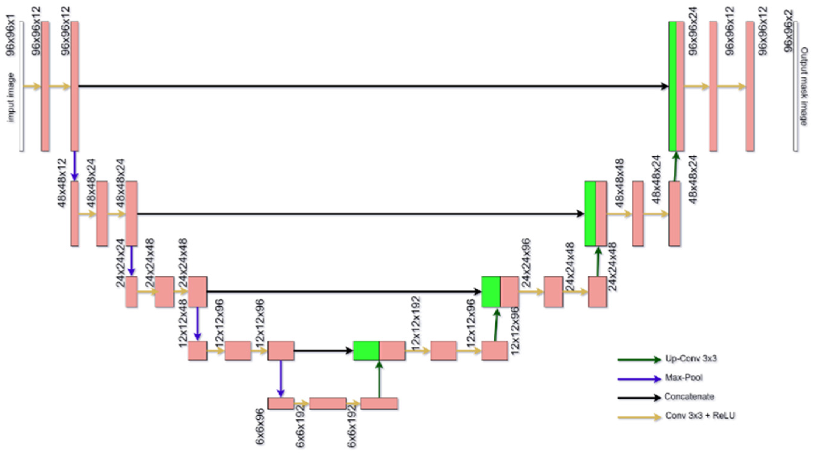
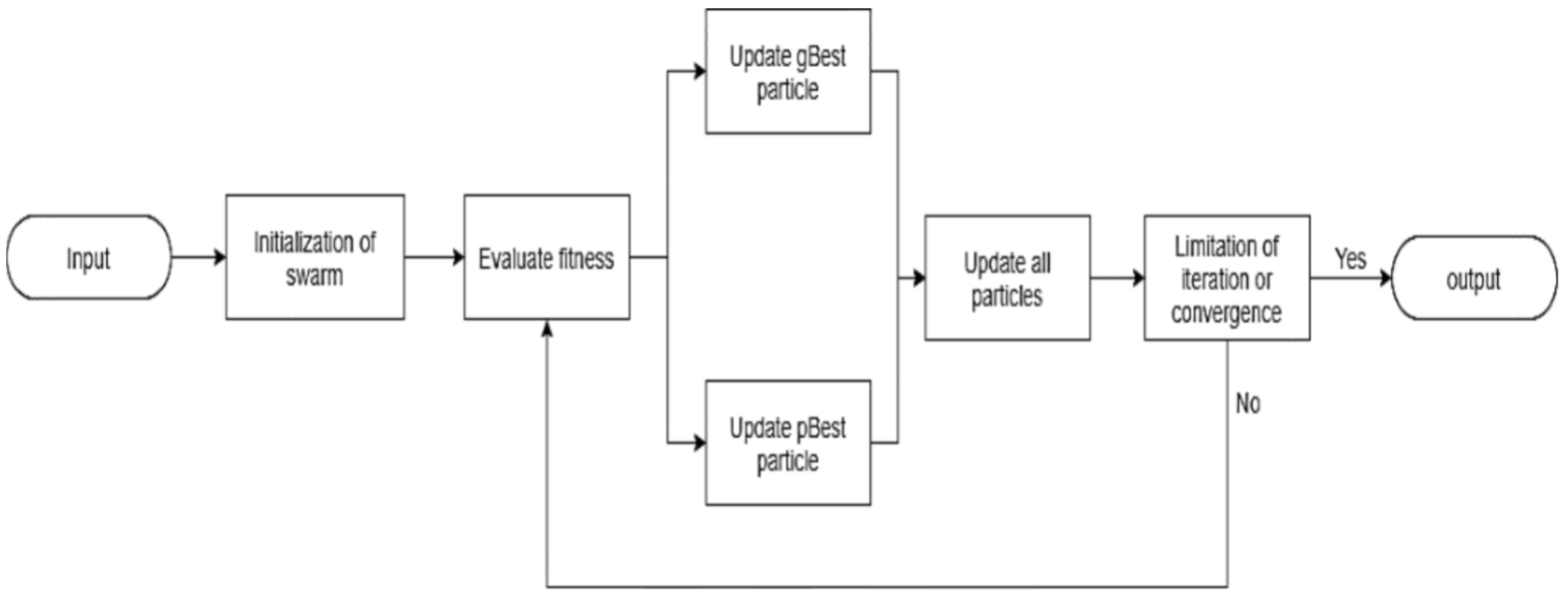
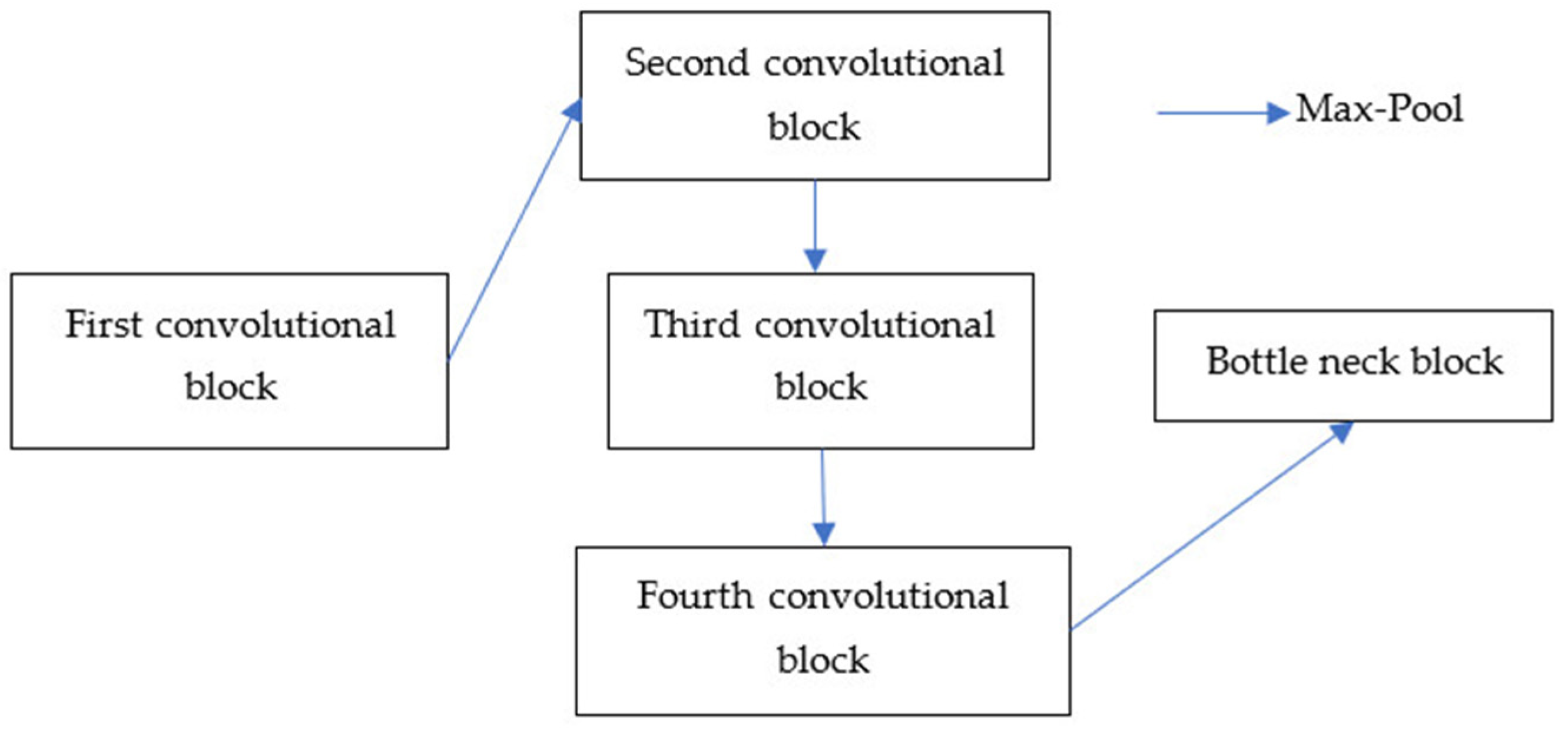
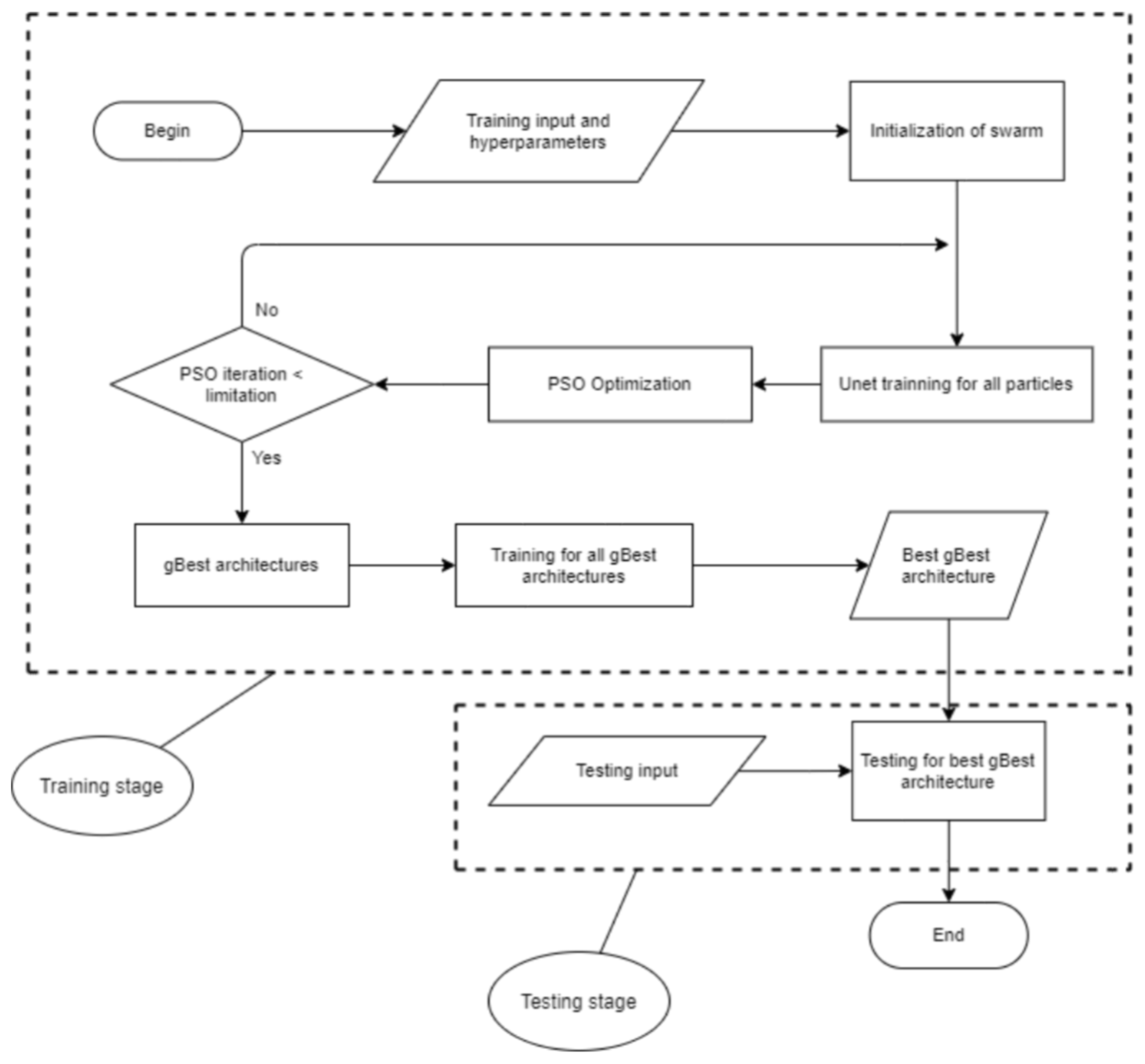
All the above-mentioned research used ML techniques to find a solution in a particular field. However, there are few articles using Deep Learning for the flash flood segmentation. In this paper, we propose a novel Deep Learning architecture, namely PSO-UNET, which combines the Particle Swarm Optimization (PSO) with the UNET model to improve the performance of the flash flood detection from satellite images. 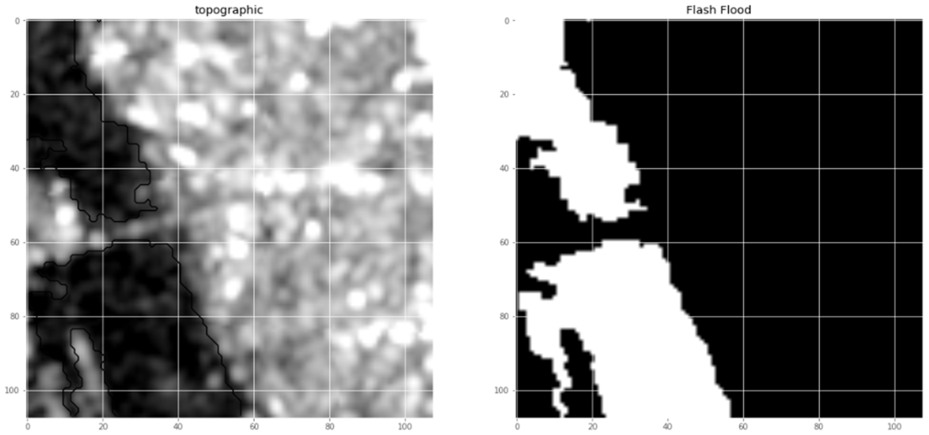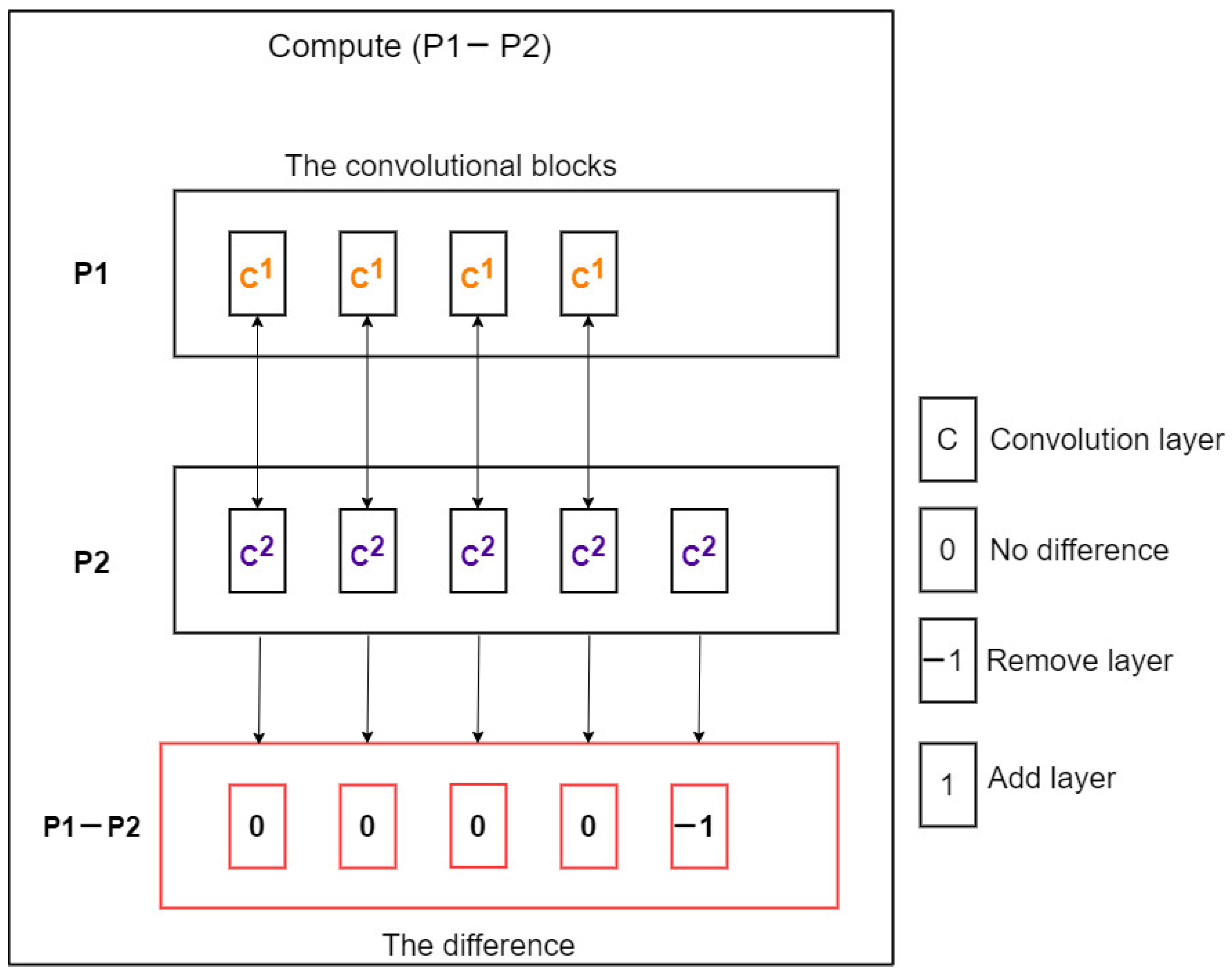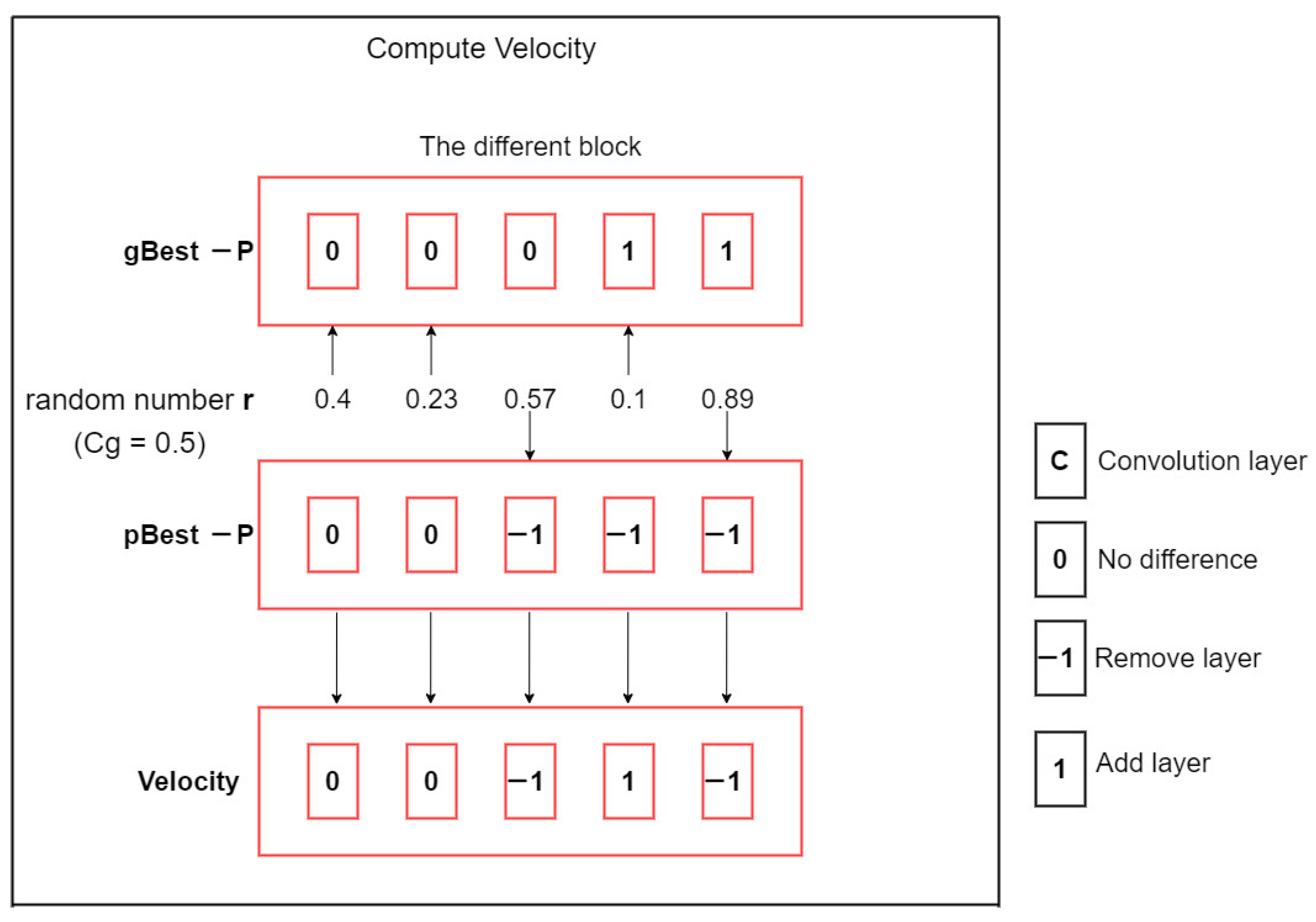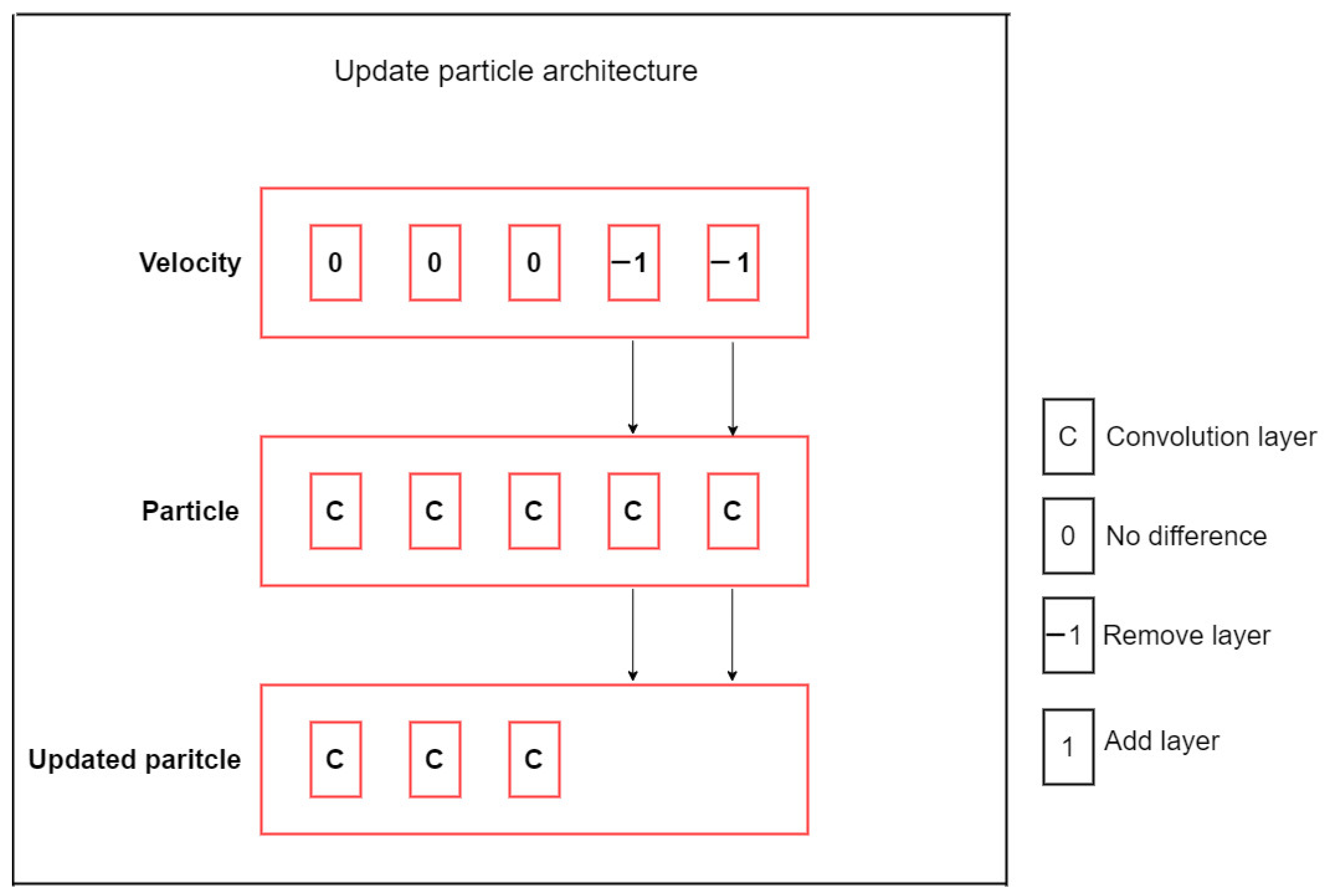UNET is a convolutional network designed for biomedical image segmentation [24]. Its architecture is symmetric and comprises of two main parts namely a contracting path and an expanding path, which can be widely seen as an encoder followed by a decoder. Since the original UNET has a symmetrical architecture, which means the expansive path is created following the contracting path, we only need to pay attention to the contracting path for the evolutionary computation. The UNET convolutional process is performed four times. Indeed, we consider each process as a block of the convolution having two convolutional layers in the original architecture. The training of inputs and hyper-parameters is performed by the PSO algorithm. By doing so, we acquire the optimal parameterization for the UNET, which is the innovative idea of this paper. Experimental results on various satellite images of Quangngai province located in Vietnam prove the advantages and superiority of the PSO-UNET approach against the original UNET.

The remainder of this paper comprises of 4 sections and is organized as follows: The UNET architecture and Particle Swarm Optimization, which are the two major components of the proposed method, are presented in Section 2. The PSO-UNET which is the combination of the UNET and the PSO algorithm is presented in detail in Section 3. In Section 4, the experimental results of the proposed method are presented. Finally, the conclusion and directions are given in Section 5.

2. Background of the Employed Algorithms

2.1. The UNET Algorithm and Architecture

The UNET’s architecture is symmetric and comprises of two main parts, a contracting path and an expanding path which can be widely seen as an encoder followed by a decoder, respectively [24]. While the accuracy score of the deep Neural Network (NN) for classification problem is considered as the crucial criteria, semantic segmentation has two most important criteria, which are the discrimination at pixel level and the mechanism to project the discriminative features learnt at different stages of the contracting path onto the pixel space.

The first half of the architecture is the contracting path (Figure 1) (encoder). It is usually a typical architecture of deep convolutional NN such as VGG/ResNet [25,26] consisting of the repeated sequence of two 3 × 3 2D convolutions [24]. The function of the convolution layers is to reduce the image size as well as bring all the neighbor pixel information in the fields into a single pixel by applying performing an elementwise multiplication with the kernel. To avoid the overfitting problem and to improve the performance of an optimization algorithm, the rectified linear unit (ReLU) activations (which expose the non-linear feature of the input) and the batch normalization are added just after these convolutions. The general mathematical expression of the convolution is described below.

$$g\left(x,y\right)=\omega \ast f\left(x, y\right)$$

(1)

where $f\left(x, y\right)$ is the original image, $\omega$ is the kernel and $g\left(x,y\right)$ is the output image after performing the convolutional computation.

Each of two 3 × 3 2D convolutions are followed by a 2 × 2 max-pooling layers down sampling with stride 2 in order to capture the context of an input image. After each down-sampling step, the spatial dimensions of the input are cut half, while the number of the feature channels is doubled. Apparently max-pooling layer helps model to extract the sharpest features of an image. Given an image, the sharpest features are the best lower-level representation of an image. Adding the max-pooling layers also help the model to reduce variance and computation complexity since 2 × 2 max-pooling layers reduces 75% data.

The expanding path (decoder) is the second half of the architecture diagram. After each 2 × 2 2D up-convolution, there is a concatenation of the feature map with a corresponding layer from the contracting path and two 3 × 3 2D convolutions, each followed by the batch normalization and the ReLU activation [24]. The main purpose of the concatenation procedure is to provide localization information due to the loss of border pixels after every convolution layer. The final layer is 1 × 1 2D convolution, which is used to map the final feature map with the desired number of classes (mask images).

The UNET architecture has robust effectiveness in the field of semantic segmentation, but the model is proved to be suitable for the medical dataset and is not appropriate fully for other datasets such as the satellite image dataset with the number of layers of the designed architecture. This paper will put forward the improvement based on this network and the classic optimization algorithm called PSO. The proposed method will be presented in the next section after summarizing the PSO algorithm.

2.2. Particle Swarm Optimization

Since the traditional convolutional neural network such as UNET for solving the problem involving in segmentation did not clearly define the reasons of choosing the number of layers and the layer’s parameters, Particle Swarm Optimization (PSO) [24] will help to seeking the most suitable one. PSO [27] is a popular technique serving several scientific fields in recent years and comparable to Genetic Algorithms (GA) [28,29] in the field of optimization. The inspiration of the PSO algorithm originated from the behavior of flocks of birds and schools of fish. The authors who originally introduced PSO [27] considered every single bird as a particle and the population of birds as swarm; thus, it is the reason why this algorithm is called the Particle Swarm Optimization. All flying birds would disperse, concentrate and after every concentration, they would adjust the directions of their flight. They also observed that the flying pace of all birds always remain stable and the changes of the flying directions is affected by its “best” reached position and group “best” position. Every single particle has its own position, its velocity at the moment, the “best” reached position and the group “best” position. After every iteration, each particle will modify its position according to its new velocity by applying the following equation:

$$v_i^{t+1}=\omega v_i^t+c_1{r}_1\left(xBes{t}_i^t-x_i^t\right)+c_2{r}_2\left(gBes{t}_i^t-x_i^t\right)$$

(2)

$$x_i^{t+1}=x_i^t+v_i^t\times t$$

(3)

where r₁ and r₂ are two random parameters within [0, 1], c₁ and c₂ are the constants, and w is the inertia weight. The flowchart of the PSO algorithm is demonstrated in Figure 2.

In order to leverage the robust ability of the PSO algorithm in the segmentation, the method presented in this paper based on the PSO would be put forward to optimize the UNET architecture and result in a higher performance with the specific dataset. Consequently, Section 4 presents in detail the proposed improved UNET architecture optimized by PSO algorithm.

3. Proposed Particle Swarm Intelligence Optimized UNET Deep Learning (PSO-UNET) for Flash Flood Detection

3.1. Preparation of the Training, Validation and Testing Dataset

The proposed UNET model is applied for 984 (108 × 108 pixels) Sentinel—2 satellite images of the dataset from the Quangngai province located in Vietnam with the coverage of the whole province of 5138 km². The images were taken from a national project in 2019. Each input image is accompanied by a corresponding fully annotated ground truth segmentation map for flash flood (white) and not flood (black). Figure 3 demonstrates a sample data image consisting of an input (left) and a mask (right) for the experimental process. Since the cost and the resource for the national project are restricted, there are various limitations of our collected dataset. For examples, the instances in the dataset only have one dimension of the 108 × 108 × 1 gray scale images, the ground truth only distinguishes from the flash flood areas and the normal areas and we could not cover the whole areas in the province.

For convenient training and testing stages, we decide to divide these images into three parts, namely train, validation and test following the K-fold Cross Validation technique with k = 3. For the 984 images, 84 images are kept as validation set and not included in the parameter selection. The K-fold applies to the train-test datasets that mean 900 images are divided to 3 folds with 300 images each and the process is repeated 3 times by keeping each fold once as test set. The qualitative results will be demonstrated in the next section.

Table 1. The preparation of experimental datasets with k = 3.

	Quantity	Size
The total image	984	108 × 108 × 1
Training dataset	600	108 × 108 × 1
Testing dataset	300	108 × 108 × 1
Validation dataset	84	108 × 108 × 1

illustrates how we divide and prepare these datasets for our experiment.

3.2. The Proposed PSO-UNET for Flash Flood Detection

Since seeking for the most suitable Deep Learning model to solve the problem of flash flood segmentation is not easy, applying PSO algorithms to optimize the number of layers in the model helps to figure out the best fit instance of the UNET-based model. Every model instance in the population (swarm) will make evolution following to the best particle by adding or removing the layers in the model. These changes have an important impact on enhance the overall performance of the instance. Finally, the best particle (the model instance) will be figured out and be trained on the whole dataset in order to find the best weights. The following subsection will describe in detail how to apply PSO algorithm into UNET deep learning model.

3.2.1. The Flow Chart of the PSO-UNET

The original UNET has a symmetrical architecture, which means that the expansive path is created symmetrically to the contracting path. Thus, we only need to pay attention to the contracting path for the evolutionary computation. The UNET convolutional process is performed four times. We consider each process as a block of the convolution having two convolutional layers in the original architecture. This specific representation is demonstrated in Figure 4.

In this representation, the max-pooling layers are fixed to a 2 × 2 filter with stride equal to 2 because it is hard to control the size of images after each convolutional block, which is randomly initialized. Another fixed layer is the bottle neck layers which has two 3 × 3 convolution layers doubling the filter of the last layer in the fourth convolutional block. In addition, we also fix the number of the convolutional blocks to four, so the evolutionary procedure of all particles cares only about comparing two convolutional blocks at the same position. The flow of the proposed method is shown in Figure 5.

In the proposed algorithm, one of the most important criteria of the PSO algorithm is the fitness function. Selecting a decent evaluation will help the algorithm reach a convergence quickly. Since each particle will have its loss function value after each iteration, comparing these values with their current best particle and global best particle is the satisfactory approach for the fitness evaluation. In our case, it is the Dice Coefficient [30] which is selected to be the fitness function for the PSO algorithm. The Dice Coefficient score is not only a measure of how many positives are found, but it also penalizes for the false positives that the method finds and be similar to precision, so it is more similar to precision than accuracy and have more suitable and significant impact on the overall performance of the optimization algorithm. The only difference is the denominator, where you have the total number of positives instead of only the positives that the method finds. So, the Dice score is also penalizing for the positives that your algorithm/method could not find. The particle having the highest score of fitness is chosen for the best architecture, which is the objective of the algorithm. In this method, the algorithm ignores the number of parameters and focuses on the best architecture to the evolution only. Therefore, these parameters do not start over.

Looking at the representation of the UNET architecture, we only need to present how to compute the velocity of the particles by comparing blocks at the corresponding position in the contracting path. The reason is that after updating the procedure, the expansive path can be created by following the contracting path so that we do not take the updated expansive path in consideration.

3.2.2. The Difference of the Convolution Blocks

In order to calculate the velocity of the specific particle, we need to represent how the difference of the two contracting paths are computed. There are four blocks in all random particles so that calculating the difference between two blocks at the same position are detailed. The others are processed similarly. Figure 6 is an example of this procedure, in which the number of convolution layer in each block is taken into consideration. Additionally, the computation is always performed with respect to the first blocks. The difference will be zero at the same position that two blocks have the presence of the convolution layer. It means these position in the block will be kept with its corresponding hyper-parameters at the updating procedure. If the first block has less (more) ‘t’ number of layers than the second, the number of −−1 (+1) added to the difference will be ‘t’, with the hyper-parameters of the layers of the second block.

3.2.3. The Velocity Computation of the Blocks

At each iteration, the velocity of each particle (P) is the virtual information for the evolutionary procedure. This is computed through the current particle best position (pBest) and the global best position (gBest) [27]. In order to calculate the velocity, it needs to know two differences (gBest—P) and (pBest—P), which is pointed out at the Section 3.1. As mentioned before, we only need to demonstrate the difference between two blocks at the same order in the contracting path. An overview of this procedure is shown in Figure 7 in which the two top rows are the difference blocks of (gBest—P) and (pBest—P), respectively. In the proposed method, we define initially the decision factor Cg in order to determine what layer the block of the velocity will be selected from (gBest—P) or (pBest —P). In order to achieve this proposal, we generate a random number r uniformly at [0.1). If r < Cg, the block of the velocity will choose the layer from the difference (gBest—P). Otherwise, the algorithm will select the layer and its corresponding hyper-parameters from (pBest—P) and put it in the block of the final velocity at the corresponding position [27].

3.2.4. The Particle Update of the Blocks

The procedure of updating the particle architecture is an uncomplicated and straightforward. It acts as an incentive for the current particle to reach a superior architecture in the proposed algorithm. According to the achieved velocity, each particle can upgrade by adding or removing the convolution layer in all its blocks. An instance of updating a particle with its velocity is described in the Figure 8 bellow.

3.3. The Applications of the Proposed PSO-UNET Model

In our improvement, the proposed PSO-UNET model could be applied to involve in a wide range of problems in satellite images. For instance, when images are sent from satellites which are outside from the Earth, the model can be trained and evaluated to decide volumes of rainfall in what zones. Figure 9 shows some areas where the PSO-UNET can be applied into.

Another application that can use our model directly is landslide mitigation problem which is very helpful for drivers since they will have awareness of what areas are likely to occur landslide. This means they will be safer when drive through these areas.

4. Results and Analysis

4.1. Experimental Environment

4.1.1. Experimental Implementation

In order to compare precisely and conveniently the PSO-UNET and other related networks, these models are implemented by the Keras library (see Appendix A), which is the high-level API of the Tensorflow framework in Python programming language that supports Deep Learning packages. Moreover, Matplot library is used for visualizing the results of our study. In addition, these networks are trained and tested in our available Ubuntu server with 8 Dual CPUs of DELL Intel(R) Xeon(R) CPU E5-2650 v4 @ 2.20 GHz having 30,720 KB of cache size and 16 GB of main memory.

In the training phase, the PSO-UNET uses the Adam optimization algorithm [31] for seeking the convergence point in the backward propagation. In addition, the learning rate of particles in the population are not only set equal to 0.001, but also the gbest particle uses the same learning rate with the step scheduler to reduce continuously learning rate after each epoch in the last gbest training phase.

4.1.2. Quality Assessment

The experimental results of the segmentation model will be assessed over several standard performance measures. More specifically accuracy, Intersection-Over-Union (IoU) [32] and F1 score [30] are used as quality indicators in this article. Given N = {1, 2, …, n} is a set of all pixels of all images in the test set, Y1 and Y2 are the output of the model and the given ground truth, respectively, over the set N. The IoU and F1 score is defined as follows:

$$IoU\left(Y_1,Y_2\right)=\frac{Y_1{{\displaystyle \cap }}^{ }{Y}_2}{Y_1{{\displaystyle \cup }}^{ }{Y}_2}=\frac{{{\displaystyle \sum }}_{i=1}^{n}min\left(Y_{1i},Y_{2i}\right)}{{{\displaystyle \sum }}_{i=1}^{n}max\left(Y_{1i},Y_{2i}\right)}$$

(4)

$$F_1\left(Y_1,Y_2\right)=\frac{Y_1{{\displaystyle \cap }}^{ }{Y}_2+Y_1{{\displaystyle \cap }}^{ }{Y}_2}{Y_1{{\displaystyle \cup }}^{ }{Y}_2+Y_1{{\displaystyle \cap }}^{ }{Y}_2}=\frac{2\ast {{\displaystyle \sum }}_{i=1}^{n}min\left(Y_{1i},Y_{2i}\right)}{{{\displaystyle \sum }}_{i=1}^{n}max\left(Y_{1i},Y_{2i}\right)+{{\displaystyle \sum }}_{i=1}^{n}min\left(Y_{1i},Y_{2i}\right)}$$

(5)

Another criterion is to evaluate visually the predicted images of the PSO-UNET with other compared models. In Section 5, the practical results are presented in order to point out the higher performance and quality of the proposed method.

4.1.3. Experimental Objectives

(a)

Find the best hyper-parameters of the proposed model from the mentioned satellite image dataset.

(b)

Compare the performance of the PSO-UNET with the relevant models (UNET, LINKNET and SEGNET) in terms of accuracy, IoU and F1 score in the dataset.

4.2. Determination of the Hyper-Parameters of the Model

At first, a reasonable approach is to properly select the PSO-UNET model with the best hyper-parameters consisting of three groups: particle swarm optimization, UNET architecture initialization and PSO-UNET training.

The hyper-parameters of the first category are presented in the

Table 2. The hyperparameter of the particle swarm optimization.

Description	Value
Number of iterations	10
Population size	10
Cg	0.5

comprising of three parameters: the number of iterations, the population size and Cg (it is the probability of selecting a layer of the block from the global best or the local best particle). The number of iterations control the number of times the PSO algorithm will run before reaching the optimization. The population size sets the number of particles in the swarm, which is the arbitrary UNET architecture in our case. These particles will be used in the particle swarm optimization in order to seek the best architecture before moving to the training stage. The Cg score plays a crucial role in the convergence of the PSO algorithm because the higher the Cg is set, the faster the particles will approach the global best architecture. This means that the algorithm is trapped in a local optimization architecture, so we will set Cg to 0.5 for a fair approach.

The hyper-parameters in the UNET architecture initialization stage adjust the diversity of the population consisting of the max number of the convolution layers in each block, the max number of filters in the first layer of the architecture, the kernel size of all convolution layers which is fixed to 3 × 3 and the parameter of all max pooling layers set to a 2 × 2 filter with stride 2. Since each particle has four blocks of convolution layers in the contracting path and the compilation of the expansive path will be followed symmetrically, the total number of layers are decided by choosing the number of the convolution layers in each block randomly. In order to keep the properties of the original UNET, the number of filters from the second convolution layer depend on the number of filters in the first convolution layer. Due to these reasons, we will set cases based on the max number of the convolution layer in each blocks m (this number can be chosen as 4, 5 or 6) and the max number of filters in the first convolution layer n in the interval of (this number can be set as 20, 30, 40) for our training and testing stages of the proposed model. Therefore, we have the cases presented in the

Table 3. The division of the cases for training and testing stages.

Case	m	n
4-20	4	20
4-30	4	30
4-40	4	40
5-20	5	20
5-30	5	30
5-40	5	40
6-20	6	20
6-30	6	30
6-40	6	40

as follow:

The final category of hyper-parameters is the PSO-UNET training process hyper-parameters which are illustrated in

Table 4. The hyperparameter of the PSO-UNET training process.

Description	Value
Number of epochs for evaluation	1
Number of epochs for global best	50
Dropout rate	0.05
Batch normalization	True
Batch size	32

. These hyper-parameters include the number of epochs for the evaluation stage, the number of epochs for the global best in the training process after the evaluation, the dropout rate, the selection of the batch normalization and the batch size of putting inputs through the model of all processes. The number of the epochs for the evaluation decide how many times each particle is trained through the complete dataset before taking part in the evaluation. After evaluation process, the global best particle will be trained with the number of the epochs for the global best. To avoid overfitting problems, the dropout rate and batch normalization are used between the layers of the particle.

After determining the cases, we conduct the experiment in all cases three times in order to gain accurate results. The average results of implementing this model on selected datasets in the range of hyper-parameters are presented in

Table 5. The results of the model experiment in different cases (the bold value is the best one in each column).

Case	Validation			Testing
	Acc (%)	IoU (%)	F1 (%)	Acc (%)	IoU (%)	F1 (%)
4-20	92.36	94.75	78.32	92.31	94.82	77.99
4-30	92.48	94.98	79.41	92.44	94.93	78.49
4-40	92.69	95.64	80.45	92.64	95.59	79.75
5-20	92.20	95.06	78.26	92.02	94.97	77.45
5-30	92.67	95.36	80.49	92.26	95.35	79.47
5-40	92.34	95.25	80.04	92.39	95.30	78.79
6-20	92.28	94.05	75.37	92.05	93.86	74.18
6-30	92.04	95.47	80.75	92.47	95.46	79.65
6-40	92.71	95.40	80.41	92.63	95.34	79.67

. In the validation process, while the case 6-40 reaches the highest Accuracy score (92.71%), the best IoU measure belongs to case 4-40 (95.64%) and case 6-30 has the highest score of F1 (80.75%). However, in the testing stage, all of the measures of the case 4-40 dominate over the rest of the cases. The Accuracy, IoU and F1 scores do not stand out from other cases. In particular, the F1 score which is chosen for the fitness function of the PSO algorithm acquires the score of 79.75%. Thus, we select the experimental results in testing process of the case 4-40 in order to compare with other related models.

After choosing the model with the best hyper-parameters, comparing the selected model with other former models has a vital role in the signification of the proposed model.

4.3. Model Comparison

Comparing the proposed model with related models is a necessary step in order to verify the efficient and sufficient performance. For this reason, we choose the original UNET model [24], the LINKNET model [33], the SEGNET [34] for our comparing process. The experimental results and assessments are presented in the following lines.

In Figure 10, the learning curve of the PSO-UNET model always stays in the bottom with others and shows the convergence smoothly in the training phase. This means our proposed model have the best learning strategy compared to others.

At first glance, pixel accuracy is the percentage of area that the trained model classifies precisely. In the segmentation section of computer vision field, it is notorious to demonstrate that high pixel accuracy does not always imply superior segmentation ability. In order to clearly illustrate the final segmentation result of our model, Intersection-Over-Union [29], also known as the Jaccard Index, is considered properly as a very straightforward metric in assessing semantic segmentation. For more equity, we also use F1 score [33] in order to appraise the proposed model at the high performance with other precedent models.

As shown in

Table 6. The comparison of the PSO-UNET model with other precedent models in testing stage (the bold value is the best one in each row).

Testing	PSO-UNET	UNET	LINKNET	SEGNET
Acc (%)	92.64 ± 0.44	92.10 ± 0.08	79.82 ± 2.44	89.80 ± 1.12
IoU (%)	95.59 ± 0.42	91.65 ± 1.33	68.12 ± 2.86	81.54 ± 2.86
F1 (%)	79.75 ± 5.12	71.19 ± 5.77	61.58 ± 7.62	51.46 ± 7.55

, our proposed model acquires the highest values in Acc, IoU and F1 score in the testing process. Accuracy of PSO-UNET reaches the peak of 92.64% over other models much higher than that of LINKNET (12.82% higher). IoU of PSO-UNET is a bit higher than that of UNET (about 4% higher) and very much higher than that of LINKNET (27.47% higher) and SEGNET (14.05% higher). However, the value of F1 score obtained by applying PSO-NET is a significantly higher than UNET (8.59%), much higher than SEGNET (18.17%) and very much higher than LINKNET (28.29%). Standard Deviation (S.D) of Acc and IoU computations of all models are very small (0.1%–3%) except F1 score computations of all models. The values fluctuate between 5% to 7% which is much higher when compared to Acc and IoU measure. In order to visualize the quantitative comparison obviously, we put these results of Table 6 in Figure 11.

The qualitative results of PSO-UNET, UNET, Linknet and SEGNET are presented in Figure 12 and Figure 13 on two differently particular areas of the dataset. These images are converted to “seismic” and “binary” types for the purpose of visualizing while clearing our results.

As illustrated in Figure 12 and Figure 13, we can evaluate that our proposed model has better segmentations qualitatively. The pixels forming the narrow lines are too hard to segment precisely, but our model provides superior results in testing images.

4.4. Evaluate the Strength of the Proposed Model

Finally, the one-way ANOVA (Analysis of Variances) Test is applied to the F1 score values of the previous four compared models (PSO-UNET, UNET, LINKNET, and SEGNET) in order to evaluate the strength of the proposed model. We choose the best three F1 score values (

Table 7. The best three instances of F1 score of all models used to take the ANOVA test.

Instance	PSO-UNET	UNET	LINKNET	SEGNET
1	86.24%	76.81	69.88	60.98
2	73.73%	73.50	63.38	50.92
3	79.27%	63.25	51.48	42.59

) of all models to take the test properly. The hypotheses are:

Hypotheses 1 (H1).

The proposed model is not different from the related models in terms of F1.

Hypotheses 2 (H2).

The proposed model is significantly different from the related models in terms of F1.

This scenario is presented in Figure 14 and

Table 8. The results of one-way analysis of variant over all models.

Source	SS	df	MS	F	Prob > F
Columns	1337.18	3	445.726	6.83	0.0135
Error	522.46	8	65.307
Total	1859.63	11

. Visually, the red bar of our proposed model which is the mean strength reaches the peak over all the remainder, about 79%. Additionally, there is no overlap between the blue bar and the red bar, and we infer that the PSO-UNET model is significantly different from the rest of the compared models.

Since the interquartile range of the PSO-UNET model is smallest (less than 10%) compared to other models (greater than 10%), this means that the variability of the F1 score in three scenarios are not different and falls into the lowest quartile range. The whiskers of the PSO-UNET and PSO models are also small relatively compared to others (approximately 2%). Finally, the confidence interval of our proposed model is fluctuated in the smaller range (about 16%) and stay in almost higher percentage which means the results of F1 score in all cases are not different and the PSO-UNET model have a significant improvement.

For the One-way ANOVA test, there are four units that need to be computed which are SS, df, MS, and F to reach the results Prob > F used to evaluate the proposed model. Particularly, SS represents the sum of square of all instances, df denotes the degrees of freedom, MS is the mean square error, and F is interpreted as the ratio of mean square error. The p-value (Pro > F value) indicate the probability of the event “The proposed model is significantly different from the related models”, which is the alternative hypothesis. If this probability is less than 0.05, we can infer that the alternative hypothesis is accepted. Otherwise, all the variances are the same.

The results of the One-way ANOVA test in the Table 8 show that the value p-value is equal to 0.0135 which is less than 0.05, so the alternative hypothesis is accepted.

5. Discussions

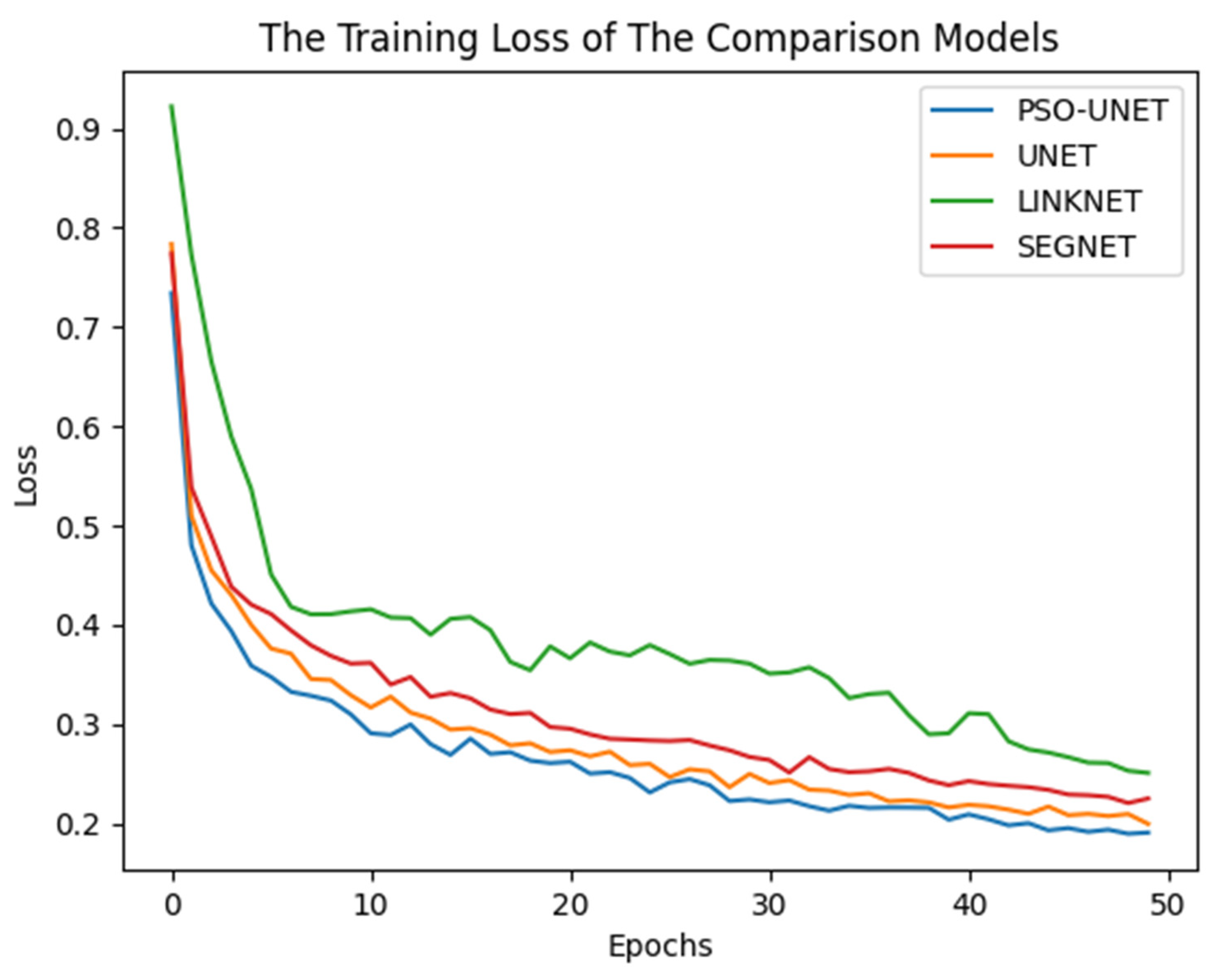
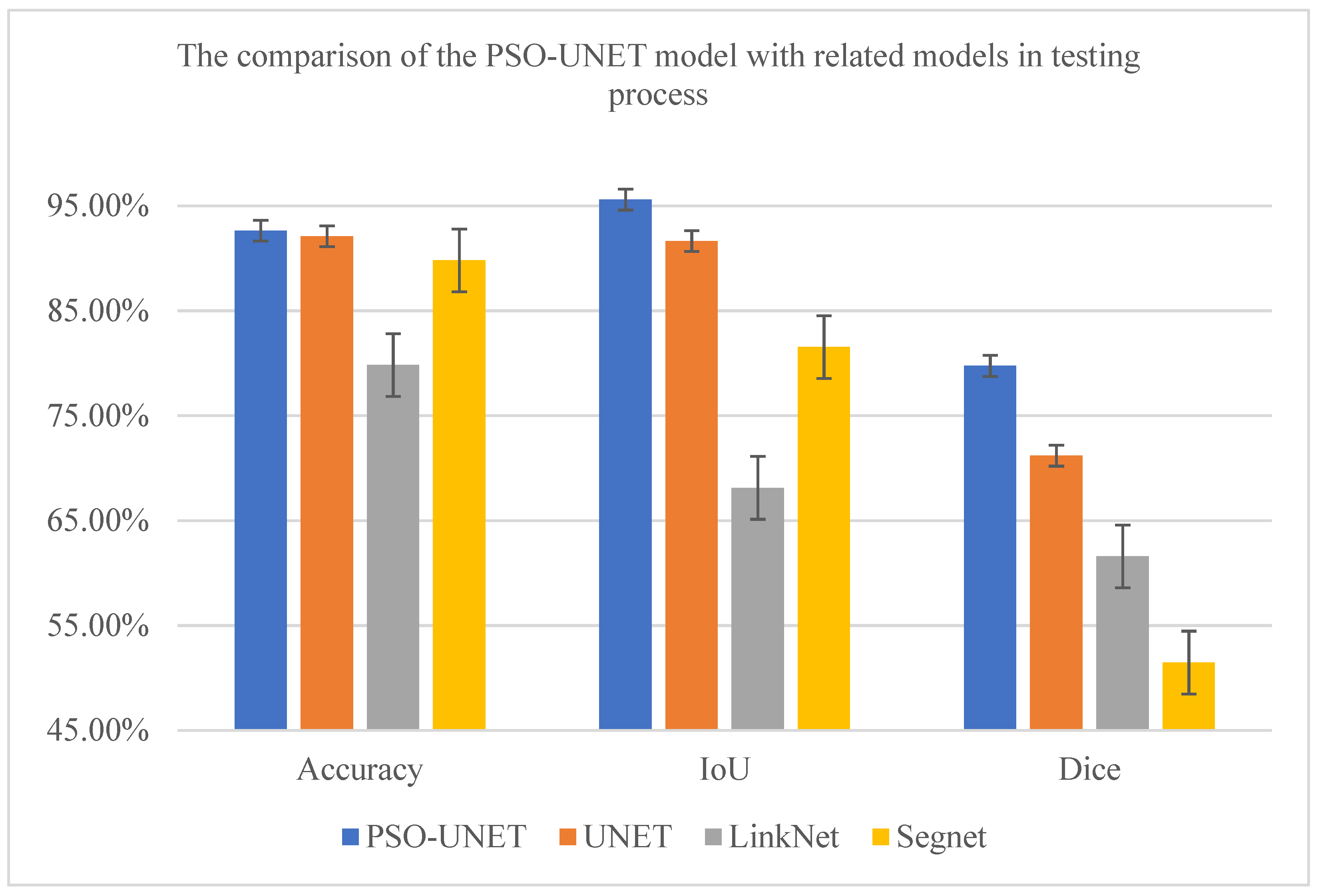
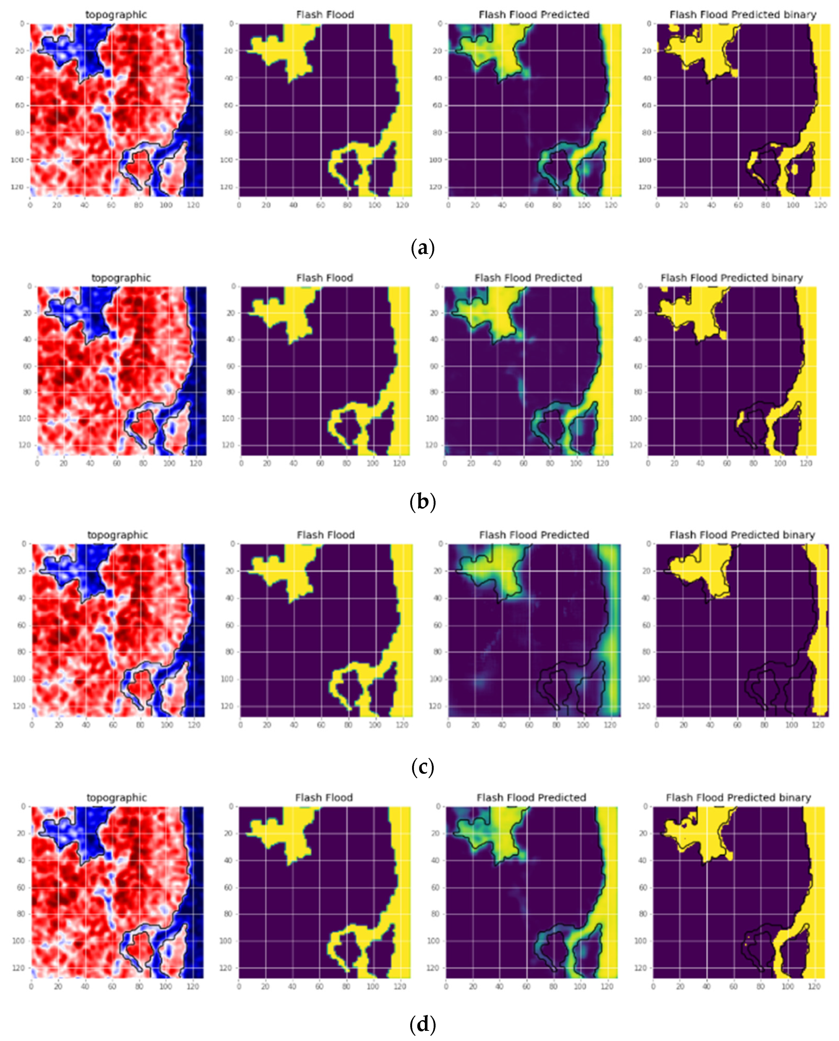
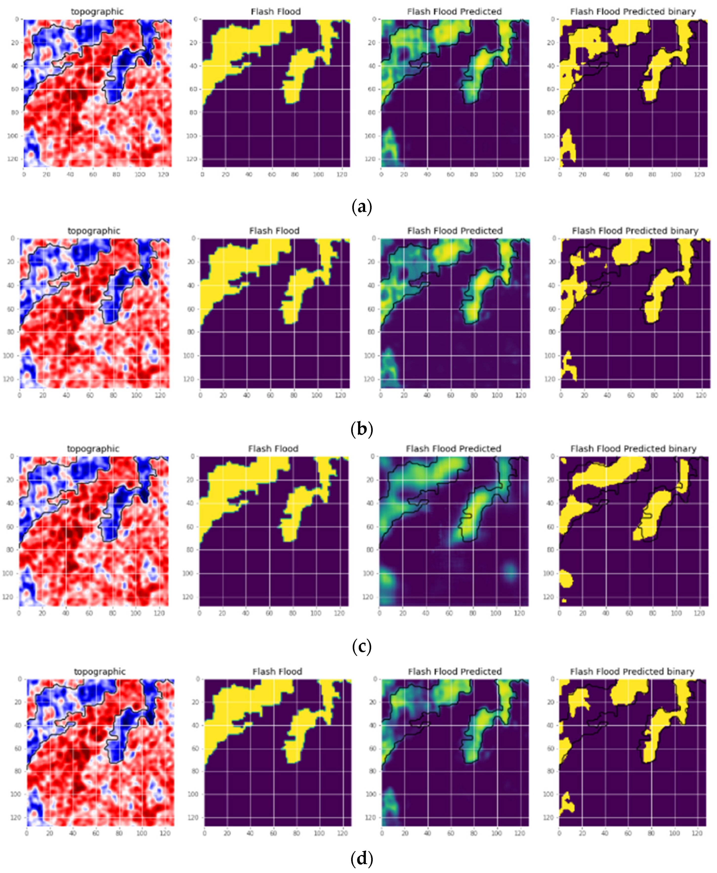
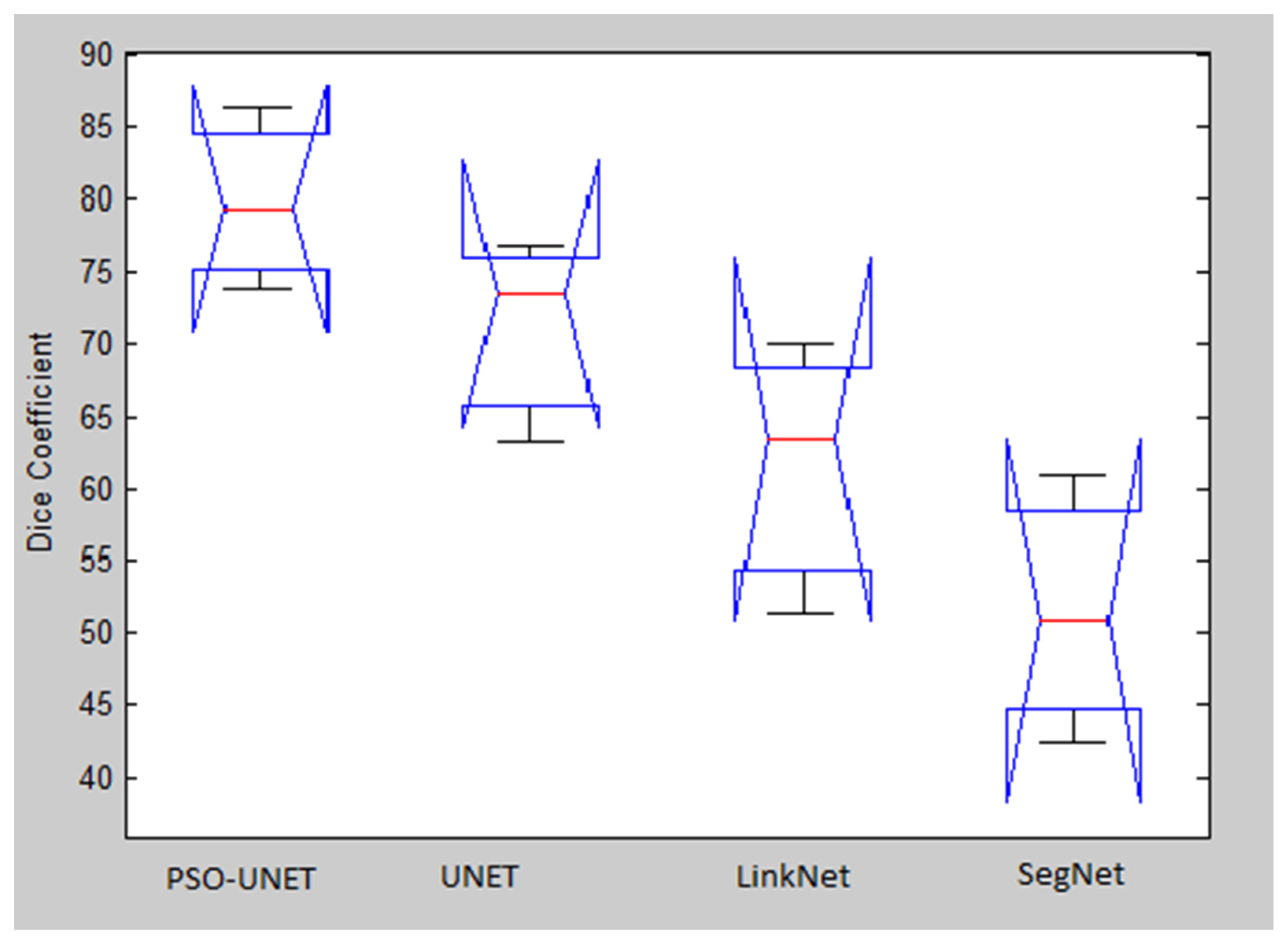
With the results presented in the previous subsections, the proposed model shows the ability and the better performance of the approach when we have experimented in the satellite images dataset. We combined the original UNET with the PSO algorithm, while the initial architectures of the UNET evolved through each iteration. These architectures approach gradually to the optimal one by adding essential layers or removing redundant layers in every convolution blocks. After each iteration, the new version of the architecture appears, so the final result has a better score when compared to related models.

In addition to these advantages, there are an existent of the time consuming in the whole training stage of the proposed model. While related models are straightforward in order to reach the best parameters of the networks, the PSO-UNET experience compulsorily through two stages of the PSO algorithm and the model training process. However, the longer running time is compensated by the better performance of all measures. For the hyper-parameters of the PSO algorithm, as the number of iterations and populations increases, the resulting architecture is better. In this paper, we just confine these hyper-parameters to improve the running time.

In the future, thanks to the unstoppable development of state-of-the-art in the computer industry, the computation speed will increase considerably, and we believe that the running time will be further improved.

6. Conclusions

In this paper, we proposed the improvement of the UNET model based on one of the most popular evolution algorithms called Particle Swarm Optimization algorithm (PSO). By combining PSO algorithm in optimizing the architecture of the UNET model, we found the best hyper-parameters in order to obtain the satisfactory results in the experimental dataset. The dataset of satellite images is gathered and collected by name of dataset’s authors thanks to the huge efforts of experiment. The dataset which consists of 984 images are experimented with the proposed model and other related models (UNET [24], LINKNET [32], SEGNET [33]) to reach the remarkable results. Thanks to the characteristic of the segmentation method and the dataset, we select the F1 score [31] as the main evaluation method accompanied with IoU [30] and Accuracy measures. Our proposed model results in an F1 score of 87.17% ± 0.36% which is a significantly higher than corresponding scores observed in the compared models.

However, there still exist pixels that the proposed model miss-segmentation due to the very closely related features. In order to overcome this challenge, we will implement the proposed model with different post processing methods down the road for the upcoming improvements. Moreover, we need to apply the model with different datasets to verify the reliability of the results and the ability of the PSO-UNET model.

References

1. Ritter, J.; Berenguer, M.; Corral, C.; Park, S.; Sempere-Torres, D. ReAFFIRM: Real-time Assessment of Flash Flood Impacts—A Regional high-resolution Method. Environ. Int. 2020, 136, 105375. [Google Scholar] [CrossRef]
2. Kankanamge, S.L.; Mendis, P.; Ngo, T. Use of fluid structure interaction technique for flash flood impact assessment of structural components. J. Flood Risk Manag. 2019, 13, e12581. [Google Scholar] [CrossRef]
3. Dano, U.L. Flash Flood Impact Assessment in Jeddah City: An Analytic Hierarchy Process Approach. Hydrology 2020, 7, 10. [Google Scholar] [CrossRef] [Green Version]
4. Sahoo, G.; Ray, C.; De Carlo, E. Use of neural network to predict flash flood and attendant water qualities of a mountainous stream on Oahu, Hawaii. J. Hydrol. 2006, 327, 525–538. [Google Scholar] [CrossRef]
5. Heiser, M.; Scheidl, C.; Eisl, J.; Spangl, B.; Hübl, J. Process type identification in torrential catchments in the eastern Alps. Geomorphology 2015, 232, 239–247. [Google Scholar] [CrossRef]
6. Sudhishri, S.; Kumar, A.; Singh, J.K. Comparative evaluation of neural network and regression based models to simulate runoff and sediment yield in an outer Himalayan watershed. J. Agric. Sci. Technol. 2016, 18, 681–694. [Google Scholar]
7. Jimeno-Sáez, P.; Senent-Aparicio, J.; Pérez-Sánchez, J.; Pulido-Velazquez, D.; Cecilia, J.M. Estimation of Instantaneous Peak Flow Using Machine-Learning Models and Empirical Formula in Peninsular Spain. Water 2017, 9, 347. [Google Scholar] [CrossRef] [Green Version]
8. Hong, W.-C. Rainfall forecasting by technological machine learning models. Appl. Math. Comput. 2008, 200, 41–57. [Google Scholar] [CrossRef]
9. Khosravi, K.; Pham, B.T.; Chapi, K.; Shirzadi, A.; Shahabi, H.; Revhaug, I.; Prakash, I.; Bui, D.T. A comparative assessment of decision trees algorithms for flash flood susceptibility modeling at Haraz watershed, northern Iran. Sci. Total Environ. 2018, 627, 744–755. [Google Scholar] [CrossRef] [PubMed]
10. Hsu, M.-H.; Lin, S.-H.; Fu, J.-C.; Chung, S.-F.; Chen, A.S. Longitudinal stage profiles forecasting in rivers for flash floods. J. Hydrol. 2010, 388, 426–437. [Google Scholar] [CrossRef] [Green Version]
11. Sharma, P.; Alshheri, M.; Sharma, R.; Alfarraj, O. Self-Management of Low Back Pain Using Neural Network. Comput. Mater. Contin. 2021, 66, 885–901. [Google Scholar] [CrossRef]
12. Wang, J.; Ma, Y.; Zhang, L.; Gao, R.X.; Wu, D. Deep learning for smart manufacturing: Methods and applications. J. Manuf. Syst. 2018, 48, 144–156. [Google Scholar] [CrossRef]
13. Helbing, G.; Ritter, M. Deep Learning for fault detection in wind turbines. Renew. Sustain. Energy Rev. 2018, 98, 189–198. [Google Scholar] [CrossRef]
14. Wang, H.; Lei, Z.; Zhang, X.; Zhou, B.; Peng, J. A review of deep learning for renewable energy forecasting. Energy Convers. Manag. 2019, 198, 111799. [Google Scholar] [CrossRef]
15. Qiao, J.; Wang, G.; Li, W.; Chen, M. An adaptive deep Q-learning strategy for handwritten digit recognition. Neural Netw. 2018, 107, 61–71. [Google Scholar] [CrossRef]
16. Fujiyoshi, H.; Hirakawa, T.; Yamashita, T. Deep learning-based image recognition for autonomous driving. IATSS Res. 2019, 43, 244–252. [Google Scholar] [CrossRef]
17. Yan, M.; Li, M.; He, H.; Peng, J. Deep learning for vehicle speed prediction. Energy Procedia 2018, 152, 618–623. [Google Scholar] [CrossRef]
18. Wason, R. Deep learning: Evolution and expansion. Cogn. Syst. Res. 2018, 52, 701–708. [Google Scholar] [CrossRef]
19. Anbarasan, M.; Muthu, B.; Sivaparthipan, C.B.; Sundarasekar, R.; Kadry, S.; Krishnamoorthy, S.; Dasel, A.A. Detection of flood disaster system based on IoT, big data and convolutional deep neural network. Comput. Commun. 2020, 150, 150–157. [Google Scholar] [CrossRef]
20. Singh, A.; Singh, K.K. Satellite image classification using Genetic Algorithm trained radial basis function neural network, application to the detection of flooded areas. J. Vis. Commun. Image Represent. 2017, 42, 173–182. [Google Scholar] [CrossRef]
21. Du, W.; Chen, N.; Yuan, S.; Wang, C.; Huang, M.; Shen, H. Sensor web—Enabled flood event process detection and instant service. Environ. Model. Softw. 2019, 117, 29–42. [Google Scholar] [CrossRef]
22. Martinez-Garcia, M.; Zhang, Y.; Suzuki, K. Deep Recurrent Entropy Adaptive Model for System Reliability Monitoring. IEEE Trans. Ind. Inform. 2020, 17, 839–848. [Google Scholar] [CrossRef]
23. Martínez-García, M.; Zhang, Y.; Gordon, T. Memory Pattern Identification for Feedback Tracking Control in Human–Machine Systems. Hum. Factors J. Hum. Factors Ergon. Soc. 2019, 63, 210–226. [Google Scholar] [CrossRef] [Green Version]
24. Ronneberger, O.; Fischer, P.; Brox, T. U-Net: Convolutional Networks for Biomedical Image Segmentation. In International Conference on Medical Image Computing and Computer-Assisted Intervention; Springer: Cham, Switzerland, 2015; pp. 234–241. [Google Scholar] [CrossRef] [Green Version]
25. Simonyan, K.; Zisserman, A. Very deep convolutional networks for large-scale image recognition. arXiv 2014, arXiv:1409.1556. [Google Scholar]
26. He, K.; Zhang, X.; Ren, S.; Sun, J. Deep Residual Learning for Image Recognition. In Proceedings of the IEEE Conference on Computer Vision and Pattern Recognition, Las Vegas, NV, USA, 27–30 June 2016; Available online: http://openaccess.thecvf.com/content_cvpr_2016/html/He_Deep_Residual_Learning_CVPR_2016_paper.html (accessed on 20 September 2021).
27. Kennedy, J.; Eberhart, R. Particle Swarm Optimization. In Proceedings of the ICNN’95-International Conference on Neural Networks, Perth, WA, Australia, 27 November–1 December 1995; Available online: https://0-ieeexplore-ieee-org.brum.beds.ac.uk/abstract/document/488968 (accessed on 20 September 2021).
28. Davis, L. Handbook of Genetic Algorithms; Van Nostrand Reinhold: New York, NY, USA, 1991. [Google Scholar]
29. Sharma, P.; Saxena, K. Application of fuzzy logic and genetic algorithm in heart disease risk level prediction. Int. J. Syst. Assur. Eng. Manag. 2017, 8, 1109–1125. [Google Scholar] [CrossRef]
30. Tiep, V.H. The Base of Machine Learning, 1st ed.; Science and Technics Publishing House: Hanoi, Vietnam, 2018. [Google Scholar]
31. Kingma, D.P.; Ba, J. Adam: Amethod for stochastic optimization. arXiv 2014, arXiv:1412.6980. [Google Scholar]
32. Real, R.; Vargas, J.M. The probabilistic basis of Jaccard’s index of similarity. Syst. Biol. 1996, 45, 380–385. [Google Scholar] [CrossRef]
33. Chaurasia, A.; Culurciello, E. LinkNet: Exploiting encoder representations for efficient semantic segmentation. In Proceedings of the 2017 IEEE Visual Communications and Image Processing (VCIP), St. Petersburg, FL, USA, 10–13 December 2017; pp. 1–4. [Google Scholar] [CrossRef] [Green Version]
34. Badrinarayanan, V.; Kendall, A.; Cipolla, R. SegNet: A Deep Convolutional Encoder-Decoder Architecture for Image Segmentation. IEEE Trans. Pattern Anal. Mach. Intell. 2017, 39, 2481–2495. [Google Scholar] [CrossRef]
Figure 1. The UNET architecture.
Mathematics 09 02846 g001
Figure 2. Flowchart of the PSO algorithm.
Mathematics 09 02846 g002
Figure 3. Sample data input of our dataset for experimental process.
Mathematics 09 02846 g003
Figure 4. The representation of the left layer of the UNET architecture.
Mathematics 09 02846 g004
Figure 5. Flowchart of the proposed method.
Mathematics 09 02846 g005
Figure 6. An example of computing the difference between two convolution blocks.
Mathematics 09 02846 g006
Figure 7. The velocity computation of two blocks.
Mathematics 09 02846 g007
Figure 8. An example of updating a particle according to its velocity.
Mathematics 09 02846 g008
Figure 9. The PSO-UNET model applications.
Mathematics 09 02846 g009
Figure 10. The comparison of the loss convergence in the training phase.
Mathematics 09 02846 g010
Figure 11. The quantitative comparison of the experimental models.
Mathematics 09 02846 g011
Figure 12. The example of the qualitative experiment of the models. (a) PSO-UNET; (b) UNET; (c) LINKNET; (d) SEGNET.
Mathematics 09 02846 g012
Figure 13. The example of the qualitative experiment of the models. (a) PSO-UNET; (b) UNET; (c) LINKNET; (d) SEGNET.
Mathematics 09 02846 g013
Figure 14. Analysis of one-way ANOVA for all models.
Mathematics 09 02846 g014