
Staggered Semi-Implicit Hybrid Finite Volume/Finite Element Schemes for Turbulent and Non-Newtonian Flows


1
Departamento de Matemática Aplicada a la Ingeniería Industrial, Universidad Politécnica de Madrid, José Gutierrez Abascal 2, 28006 Madrid, Spain
2
Laboratory of Applied Mathematics, DICAM, University of Trento, Via Mesiano 77, 38123 Trento, Italy
*
Author to whom correspondence should be addressed.
Mathematics 2021, 9(22), 2972; https://0-doi-org.brum.beds.ac.uk/10.3390/math9222972
Submission received: 24 October 2021
/
Revised: 18 November 2021
/
Accepted: 19 November 2021
/
Published: 21 November 2021
(This article belongs to the Special Issue Computational Methods in Nonlinear Analysis and Their Applications)
Abstract
:This paper presents a new family of semi-implicit hybrid finite volume/finite element schemes on edge-based staggered meshes for the numerical solution of the incompressible Reynolds-Averaged Navier–Stokes (RANS) equations in combination with the turbulence model. The rheology for calculating the laminar viscosity coefficient under consideration in this work is the one of a non-Newtonian Herschel–Bulkley (power-law) fluid with yield stress, which includes the Bingham fluid and classical Newtonian fluids as special cases. For the spatial discretization, we use edge-based staggered unstructured simplex meshes, as well as staggered non-uniform Cartesian grids. In order to get a simple and computationally efficient algorithm, we apply an operator splitting technique, where the hyperbolic convective terms of the RANS equations are discretized explicitly at the aid of a Godunov-type finite volume scheme, while the viscous parabolic terms, the elliptic pressure terms and the stiff algebraic source terms of the model are discretized implicitly. For the discretization of the elliptic pressure Poisson equation, we use classical conforming and finite elements on triangles and rectangles, respectively. The implicit discretization of the viscous terms is mandatory for non-Newtonian fluids, since the apparent viscosity can tend to infinity for fluids with yield stress and certain power-law fluids. It is carried out with finite elements on triangular simplex meshes and with finite volumes on rectangles. For Cartesian grids and more general orthogonal unstructured meshes, we can prove that our new scheme can preserve the positivity of k and . This is achieved via a special implicit discretization of the stiff algebraic relaxation source terms, using a suitable combination of the discrete evolution equations for the logarithms of k and . The method is applied to some classical academic benchmark problems for non-Newtonian and turbulent flows in two space dimensions, comparing the obtained numerical results with available exact or numerical reference solutions. In all cases, an excellent agreement is observed.
1. Introduction
The study of the incompressible Navier–Stokes equations has started many decades ago, motivated by the necessity of modelling numerous industrial processes and natural phenomena. However, more recently, with the growing development of high-performance supercomputers, numerical methods have become essential for its solution. Even if nowadays we account for a large number of well-established approaches, including different kinds of finite differences (FD), finite volumes (FV), and finite element (FE) methods, the numerical solution of incompressible flows is still a very active field of research.
According to the time discretization approach, we can divide most numerical methods for time-dependent PDEs among explicit and implicit approaches. Explicit methods directly compute the solution at a new time step from the previous one, but the allowed time step is limited by a CFL-type condition that is necessary for the stability of the scheme. On the other hand, fully implicit schemes allow in principle the use of arbitrarily large time steps, only bounded by accuracy and resolution requirements for the problem consideration, but require the solution of complex nonlinear systems. Trying to keep the best of each approach, semi-implicit schemes have been developed, showing an excellent performance for the solution of many PDE systems using either FD [1,2,3,4,5,6], FV [6,7,8,9,10,11,12,13] or continuous and discontinuous Galerkin FE methods [14,15,16,17,18,19].
Focusing on the numerical solution of the incompressible Navier–Stokes equations, a classical approach consists of applying an operator splitting strategy decoupling the computation of momentum and pressure variables [1,20,21,22]. Consequently, we can end up with a hyperbolic dominated subsystem for the velocity unknown and a Poisson problem for the pressure. If we now take into account that explicit FV methods are well suited for solving hyperbolic equations and implicit FE methods are well known to be suitable and efficient for the solution of elliptic Poisson-type problems, we will end up with a hybrid FV/FE methodology that solves each subproblem with the most suitable scheme. The operator splitting between pressure-independent purely convective terms and pressure terms can also be extended to the compressible case, see [23,24,25,26,27,28], keeping a reasonable time step restriction depending only on the velocity field, rather than on the sound speed.
Let us note that, despite turbulence playing an important role in many industrial applications, such as in the automotive and aerospace industry, most of the aforementioned schemes have been proposed in the context of laminar flows. Similarly, the Newtonian behavior of the fluid is a general assumption when addressing incompressible flows. However, there are many natural processes in which non-Newtonian fluids need to be considered, like blood and lava flows, or when studying the behavior of different materials, like toothpaste or honey. A common challenge between these two kinds of flows is the increasing complexity and weight of viscous terms with respect to the convective terms that usually dominate the incompressible Navier–Stokes equations. A careful discretization of the governing PDE system is therefore needed, which is able to deal with both low and high Reynolds number flows. In this paper, we aim at extending the hybrid FV/FE methodology presented in the series of papers [27,28,29,30,31,32], to the case of turbulent flows and non-Newtonian power-law fluids with yield stress.
To deal with turbulent flows, we consider the Reynolds averaged Navier–Stokes (RANS) system coupled with the turbulence model [33], a classical approach providing good results while keeping a low computational cost. Accordingly, the RANS equations are enlarged with two extra advection-diffusion-reaction equations for the turbulent kinetic energy k and the energy dissipation rate , coupled with the momentum conservation equation through the viscous stress tensor. Let us note that one of the major difficulties of the new pair of PDEs is the numerical treatment of the algebraic source terms that depend on the flow variables and may become highly stiff. To overcome this issue, we will define an ODE subsystem whose solution will be used to update the advection-diffusion equations and that perfectly adjusts to the operator splitting strategy used in this paper. Following the seminal ideas in [34,35,36,37], instead of working directly with the turbulence variables k and , we will make use of an ODE subsystem based on its logarithmic counterparts so that the positivity preserving property of k and is essentially verified by construction. For a certain class of methods, we are even able to prove strict positivity preservation in each substep of the scheme. This is crucial for the algorithm to provide physically consistent solutions [38,39,40], and is often also called realizable turbulence model.
From the rheology point of view, we focus on the so-called Herschel–Bulkley fluids [41]. The corresponding model is a generalization of the power-law model, which includes the yield stress and a non-linearity of the shear stress, and that have Newtonian and Bingham [42] fluids as special sub-cases. We then need to deal with the discontinuity in the rheological behavior of the flow arising from the presence of the yield stress. In the literature, there are two main ways of overcoming this issue: the first one is a variational reformulation using multipliers and combining the constitutive law with the momentum equation [43,44,45], and the second one is the regularization of the constitutive law [46,47,48,49]. In this paper, we choose the second option, i.e., we regularize the constitutive model taking into account the regularization proposed in [49]. Further advances in the simulation of non-Newtonian fluids in the framework of Stokes and Navier–Stokes equations can be found in [48,50] and of the GPR model for continuum mechanics in [51,52].
As already mentioned, one of the most significant numerical difficulties that we encounter when addressing turbulence and non-Newtonian fluids is the time step restriction that may result in an explicit discretization of the viscous terms. Therefore, differently from what has been done in former hybrid FV/FE methods [53], we will apply operator splitting again to define two subsystems. The first one contains the advection terms and will be solved explicitly. Meanwhile, the viscous subsystem will be treated implicitly. Consequently, the CFL condition of the explicit part of the scheme does not depend on the diffusion terms and allows larger time steps than a completely explicit discretization. In fact, this combination of implicit/explicit schemes to solve advection-diffusion equations is a classical approach used to take advantage of the strengths of both FV and FE methods in mixed schemes. The usual procedure for combining them is to consider a finite volume scheme for the approximation of convective terms while diffusion is handled by a continuous or discontinuous Galerkin finite element approach. Many examples can be found in the literature, including both collocated [40,54,55] and staggered grids [56,57,58]. Furthermore, theoretical analysis for this kind of combined FV-FE methods, applied to general advection-diffusion-reaction equations or the particular case of Navier–Stokes equations, is also available, see for instance [59,60,61,62].
Another important point that we have not raised yet is the spatial discretization of the 2D computational domain. We will consider two grid arrangements: unstructured simplex meshes and Cartesian grids for the finite element method. In both cases, edge-based dual grids will be generated for the finite volume scheme. Apart from the location of the discrete unknowns, one of the main differences between the algorithms proposed for the two kinds of meshes is how diffusion is addressed. If the domain is discretized by means of unstructured grids, in this paper we will use implicit continuous finite elements, while implicit finite volumes are chosen for Cartesian grids.
To attain a second order finite volume scheme on unstructured grids, a local ADER methodology is used. Furthermore, in this context, we take advantage of the dual mesh structure, and a Galerkin approach is employed for the computation of the gradients needed in the reconstruction and half-in-time evolution steps [63,64]. Further details on the classical ADER approach are presented in [65,66,67,68,69], and the modern ADER-DG methodology can be found, for instance, in [70,71]. For a more comprehensive review of the latest advances in this field, we refer to [72,73]. Regarding the Cartesian-based algorithm, the classical MUSCL-Hancock method is employed [74,75].
The rest of the paper is organized as follows. In Section 2, we present the governing equations and introduce the proposed flux splitting. Section 3 is devoted to the numerical method. We first concentrate on the case of unstructured grids recalling the computation of convection terms using explicit FV. Then, we introduce the implicit algorithm for viscous terms and define the weak problem associated with the pressure subsystem. The interpolations used to pass data between the staggered grids are provided, and the identity interpolation property is proven. The second part of the section focuses on the novel hybrid FV/FE algorithm on staggered non-uniform Cartesian grids. Again, all stages are detailed, highlighting the differences with respect to the scheme on unstructured meshes. Furthermore, the positivity preserving discretization of the source terms of the model using an ODE system based on the time evolution of the logarithms of k and is described, and the positivity preserving property on orthogonal grids is rigorously demonstrated for each substep of the scheme. The validation of the proposed methods is carried out in Section 4. Several numerical test cases for both, non-Newtonian fluids and simple turbulent flows are presented, and the obtained numerical results are compared against available analytical and numerical reference solutions. Finally, in Section 5, the main conclusions and an outlook are drafted.
2. Governing Partial Differential Equations
In this paper, we consider the incompressible Reynolds-Averaged Navier–Stokes (RANS) equations with the k − turbulence model that consist of the mass and momentum conservation laws and the evolution equations for the turbulence quantities k and . The mathematical model for incompressible flows, written in terms of conservative variables, reads
where is the constant fluid density, is the velocity vector, p is the pressure, k is the turbulent kinetic energy, the turbulent dissipation rate and the shear stress tensor is given by
where denotes the laminar viscosity and the turbulent viscosity. The production term in (3) depends on the velocity gradient and reads
Throughout this paper, we will make use of the following notation for the vector of conservative variables: , which allows rewriting the evolutionary part of the PDE system, i.e., (2)–(4), in more compact form as
Here, the convective flux tensor contains the hyperbolic part of the PDE system (2)–(4), while the parabolic terms are in the viscous flux tensor . Furthermore, is the flux tensor due to the pressure, and is the algebraic source term corresponding to the right-hand side of (2)–(4). While the definition of the stress tensor (5) is universal in this paper, the rheology for calculating the viscosity depends on the nature of the flow. More precisely, we consider either laminar non-Newtonian flows or turbulent Newtonian flows. In principle, also a combination of both is straightforward, but later we want to compare with existing results from classical test problems that are available in the literature for each flow rheology separately, and therefore this topic is left to future research. Below, we describe both the laminar non-Newtonian rheology, as well as the turbulent Newtonian one. Throughout this paper the international system of units (SI) is employed. The governing equations are presented for the most general case in three space dimensions, and the unstructured hybrid FV/FE method has also been implemented in 2D and 3D, see [27,28,30,31]. However, the numerical test problems shown later are restricted to the two-dimensional case, i.e., assuming planar problems with .
2.1. Laminar Non-Newtonian Fluids
In order to describe a laminar flow, it is sufficient to set the coefficients in the model (1)–(4). Furthermore, one needs to set .
For non-Newtonian fluids, the viscosity coefficient depends on the rate of shear tensor
where is the strain rate tensor. The rheology for the viscosity considered in this paper is the one of a Herschel–Bulkley fluid [76] with yield stress and reads as follows:
Here, is the so-called consistency index, is the yield stress of the fluid, and n is the power-law index which represents the deviation from Newtonian behavior. The Bingham model is a particular case of the Herschel–Bulkley (HB) model (7), where and the power-law model is a particular case where . For the viscosity in the cases where or , and this fact leads into numerical difficulties (see [77]), hence making an implicit discretization of the viscous terms mandatory. To avoid infinite viscosities, in this paper we consider the widely used regularization of Papanastasiou, proposed in [49,78]:
with the regularization constant set to . Moreover, we can define the generalized Bingham number for the HB model as
where V is a characteristic velocity, h is the characteristic length (usually the channel width) and the generalized Reynolds number can be written as (see [79,80])
2.2. Turbulent Newtonian Flows
To model turbulent flow regimes at the aid of the RANS equations with the model, i.e., with Equations (1)–(4), one chooses in general a constant molecular viscosity , while the turbulent viscosity is given by the usual relation
see also (5). The parameters for the k − model are typically chosen as , and , which are semi-empirical closure constants, and that are the turbulent Prandtl numbers.
A critical point when simulating turbulent flows is the near-wall region within turbulent boundary layers. From the numerical point of view, capturing a turbulent boundary layer correctly is very demanding and requires the use of very fine grids. Moreover, the standard model is no longer valid in the viscous sublayer very close to the wall. Nevertheless, several approaches have been developed in the literature, aiming at overcoming this issue, like wall laws and low Reynolds number turbulence models.
This work will focus on a realizable discretization of the model that assures the positivity of k and . Furthermore, we will make use of the low Reynolds number model of Lam and Bremhorst [81] that can be used to solve the entire turbulent boundary layer, from the outer region down to the wall, capturing both the viscous sublayer and the logarithmic layer.
The Lam-Bremhorst model suggests modifying the coefficients , and of the standard model based on two characteristic Reynolds numbers and that contain the distance to the wall as well as a characteristic size of the turbulent eddies, respectively. They read
The standard model coefficients , , and are then modified in terms of and and three functions , and as follows:
where
with , and the constants of the original model. Compared to the original Lam-Bremhorst model in this work the function has been slightly modified in order to guarantee the realizability condition , which will be required later.
For the Lam-Bremhorst model, the following boundary conditions are generally imposed at wall boundaries , see [82]:
i.e., homogeneous Dirichlet boundary conditions for the turbulent kinetic energy k and homogeneous Neumann boundary conditions for the turbulent dissipation rate . These boundary conditions are usually straightforward to implement in a numerical code.
2.3. Flux Splitting
As usual in the context of semi-implicit schemes [3,8,18,24,83,84,85,86], to decouple the evolution system (6) into convection, diffusion, pressure terms and algebraic source terms, the above system (1)–(4) is now split into four subsystems:
Convective subsystem
The convective (hyperbolic) subsystem,
which in this paper will be discretized explicitly, reads
Viscous subsystem
The viscous (parabolic) subsystem,
which will be discretized implicitly, reads
Pressure subsystem
The elliptic pressure subsystem
that must be discretized implicitly reads
ODE subsystem including the source terms of the turbulence model
Last but not least, the system of ODE
containing the potentially stiff algebraic source terms of the turbulence model and which requires an implicit positivity preserving time discretization, reads
3. The Hybrid Finite Volume/Finite Element Method
To solve the incompressible RANS equations in combination with the turbulence model, we extend the family of hybrid finite volume/finite element methods described in [27,28,29,30,31,32]. This methodology relies on a specific combination of explicit and implicit FV and FE methods to solve the subsystems obtained from the flux splitting introduced in the previous section. The main stages can be summarized as:
- Transport stage. The convective subsystem (13) is solved using an explicit FV method, and an intermediate approximation of the conservative variables vector is obtained.
- Viscous stage. The viscous subsystem (17) is discretized at the aid of implicit FE or FV methods.
- Interpolation stage. The intermediate states of the conservative variables are interpolated from the dual mesh to the primal one. See Section 3.1.1 and Section 3.2.1 for further details about how the staggered grids are defined.
- Projection stage. The new discrete pressure field is obtained with an implicit FE method by solving the corresponding Poisson problem that is obtained from the saddle-point problem (21) and (22).
- Post-projection stage. The intermediate approximation of the conservative variables is updated considering the solution computed on the projection stage and the contribution from the source terms of the equations.
In what follows, we describe the semi-implicit hybrid FV/FE scheme on two different kinds of computational grids: staggered unstructured simplex meshes and staggered Cartesian grids. For each of them, a description of the mesh arrangement is given, the notation is introduced, and the numerical discretization of the four subsystems is provided. Moreover, the positivity-preserving property of the discretization of the source terms in the model is proven. Throughout this section, capital letters refer to the discrete variables, and the super-index denotes intermediate approximations, that is, if the state vector is defined as then, is the discrete approximation of , and and are the intermediate approximations. For the sake of simplicity, the hybrid FV/FE method is in the following only presented in two space dimensions, but it has already been implemented as well for the unstructured three-dimensional case, see [27,28,30,31].
3.1. Unstructured Simplex Meshes
We first focus on extending the hybrid FV/FE schemes on unstructured simplex meshes to solve turbulent flows and to deal with non-Newtonian fluids. To this end, an implicit discretization of the viscous terms is proposed, and a novel numerical treatment of the k and equations is described.
3.1.1. Staggered Unstructured Grids
Let denote an unstructured triangular partition of the spatial computational domain , that is, , where are the elements of the primal mesh. From this mesh, we built a dual staggered mesh, such that the barycenters of the edges of the triangles of the primal mesh will be taken as the nodes of the elements of the dual mesh, , which are called cells (see the details in Figure 1). There are two different kinds of dual volumes: the interior cells, built by merging the two triangles formed by connecting the barycenters B and of two primal elements, that share an interior edge, with this edge (gray elements in the central and right-hand sketches of Figure 1), and the boundary cells, built connecting a boundary edge with the barycenter of the triangle to which the edge belongs (white elements in the central and right-hand sketches of Figure 1). Moreover, the following mesh-related notation needs to be defined:
- is a subset of nodes formed by the barycenters of the dual elements sharing an edge with the cell , i.e., is the set of neighbors of .
- is the area of , its boundary, and its outward unit normal.
- is the shared edge between the dual elements and , its barycenter, and its outward unit normal vector. Moreover, , where represents the length of .
3.1.2. Explicit Discretization of the Convective Terms
In the first stage, the convective subsystem (14)–(16) is discretized explicitly with a finite volume method. Integrating
on each control volume and applying the Gauss theorem, we get the intermediate approximation of the conservative variables, including the convective terms,
where is the set of neighbors of the control volume . To approximate the flux term with second order of accuracy in space and time, the Rusanov scheme [87], combined with a local ADER methodology [30], has been considered. Accordingly, the integral over the cell boundary is split into the sum of the integrals over the cell edges , and the integral on is approximated using a numerical flux function , which reads
where the Rusanov coefficient is given by
with the maximum signal speed on the edge, an optional artificial viscosity coefficient that can be used to improve the stability properties of the scheme, and are the half-in-time evolved reconstructed variables on the left and the right of the element interface, respectively, which are obtained following the local ADER approach [30].
3.1.3. Implicit Discretization of the Viscous Terms
The viscous subsystem is discretized implicitly with a finite element method. After semi-discretization in time the viscous subsystem reads
where is the intermediate solution obtained from (25), which involves only convective terms, and is the intermediate approximation including also viscous terms. Let us denote the boundary of the computational domain, , and the outward-pointing normal vector. Multiplying Equation (26) by a test function , , and integrating in , the weak formulation associated with the former system (26), after integration by parts, reads:
Weak problem 1.
Find verifying
for all .
The former weak problem is discretized using finite elements. To avoid nonlinearities, we assume a known constant viscosity coefficient per element, computed from the solution obtained at the previous time step. Hence, the resulting system can be efficiently solved using a matrix-free conjugate gradient algorithm. Let us also note that, since the value of the intermediate approximation is computed on the dual mesh, to solve (26), we need to interpolate from the dual mesh nodes to the primal mesh vertices. First, the local interpolation polynomials at each primal element passing through the barycenters of the edges are computed and evaluated on each vertex. Then, the final value on each vertex is computed as a weighted average of the values obtained at that vertex in each primal element. Further details on the properties of the employed interpolations are provided in Section 3.1.6.
3.1.4. Finite Element Discretization of the Pressure System
Once the intermediate value for the velocity field , including the convective and viscous terms, has been computed, the pressure and the final velocity fields are obtained using a projection method.
Projection stage
The semi-discrete pressure system results
Introducing (27) in Equation (28) multiplied by the constant density , yields
which can be seen as a Poisson-type problem to be solved using finite elements. Multiplication by a test function and integration over , after integration by parts leads to the following weak formulation:
Weak problem 2.
Find verifying
for all .
The algebraic system resulting from the discretization of (29) is again solved with a matrix-free conjugate gradient method.
Post-projection stage
Once the new discrete solution of the pressure has been obtained, the vector of conservative variables can be updated, taking into account that according to (27)
Let us note that the degrees of freedom of the intermediate variables and the new pressure are defined in the vertices of the primal mesh, while the conservative variables are needed in the dual control volumes of the finite volume scheme to be able to run the next time step. Therefore, we first interpolate the contribution of viscous terms to the dual nodes and then add the contribution of the pressure gradient by using a weighted average of the values obtained at the finite elements related to the dual cell.
3.1.5. Algebraic Source Terms of the Model
The contribution of source terms in the k and equations is computed solving the ODE system (23) and (24). The methodology employed is the same for both the unstructured and Cartesian-based meshes algorithms and can be found in Section 3.3, where also the positivity-preserving property is demonstrated.
3.1.6. Interpolation between Staggered Grids
When dealing with staggered grids, special attention should be paid to the interpolation technique used to minimize artificial diffusion effects that might even ruin the overall accuracy of the scheme [55]. In the hybrid FV/FE algorithm for unstructured grids, we have seen the necessity of passing data between the vertices of the primal elements and the nodes of the dual cells. The assumption of the dual nodes to be located not in the barycenter of dual cells but in the barycenter of the edges of the primal grid allow us to define a special interpolation which has the property that the interpolation between the vertices of the primal mesh and the nodes of the dual grid is exactly reversible. In other words, the data interpolation from the primal mesh to the dual grid and back to the primal mesh is the identity operator.
To show this property, we start focusing on a triangle of the primal mesh with vertices of coordinates , and edge midpoints , see Figure 2. Denoting by , and the basis functions on the reference triangle of the finite elements and being q an arbitrary variable with the values at the vertices of the primal element, then there exists a unique interpolation polynomial of degree one, , satisfying the interpolation property
which reads
We, therefore, get the following interpolation from the vertices into the edge midpoints:
corresponding to the proposed interpolation from FE vertices to FV nodes.
We now consider the backward interpolation from dual nodes to primal vertices. Given a primal element the basis functions associated with the barycenters of its edges read , , , which are the basis functions of linear Crouzeix-Raviart elements. Again, there exists a unique first order interpolation polynomial,
passing through , and . Evaluating it in the vertices of we get
Hence, the original values in the vertices are identically reproduced for any primal element selected.
Finally, denoting the set of elements containing a vertex , and choosing any set of weights such that , the value of q at each vertex of the primal mesh can be obtained as the weighted average
3.2. Cartesian Grids
To the best knowledge of the authors, this is the first time that a semi-implicit hybrid finite volume/finite element scheme is proposed on staggered Cartesian meshes, since previous work on hybrid FV/FE schemes was focused on unstructured simplex meshes in two and three space dimensions, see [27,28,30,31,32]. Here, we propose to use a staggered Cartesian mesh similar to the one used in [8,9,12,25,88]. Overall, we have three overlapping edge-based staggered meshes.
3.2.1. Staggered Cartesian Grid Configuration and Notation
In this section, the barycenters of the non-uniform Cartesian primal mesh are denoted by , and the corresponding cell size is denoted by and ; the barycenters of the staggered edge-based dual cells in direction for the velocity component u are denoted by with respective cell size and ; the barycenters of the staggered edge-based dual cells in direction for the velocity component u are denoted by with respective cell size and , see Figure 3 for clarity. The elements of the primal mesh are ; those of the edge-based staggered dual mesh in direction are denoted by , and those of the edge-based staggered mesh in direction are defined as .
The pressure field is discretized via a conforming finite element method with the pressure defined in the vertices of the primal control volumes , i.e., the pressure degrees of freedom at time are denoted by . The velocity components are defined in the edges of the primal control volumes as and , respectively. The turbulence quantities k and are defined in the barycenters of the primal mesh, i.e., and .
The interpolation of the velocity field from one mesh to another is achieved via the following simple interpolation rules whenever needed:
and
3.2.2. Explicit Discretization of the Convective Terms
If is the discrete state vector, the convective subsystem (14)–(16) is discretized using an explicit Godunov-type finite volume scheme on the main grid as follows:
with the numerical flux functions for a first order upwind scheme in x- and y-direction defined as:
and
We emphasize that here the velocities and are the normal velocity components on the edges resulting from the projection stage, i.e., from the solution of the elliptic pressure Poisson equation at the previous time step. In order to reach second order of accuracy, the boundary-extrapolated and time-evolved values of a second order TVD MUSCL-Hancock scheme can be used instead of the cell averages. The second order fluxes read
and
with the boundary extrapolated values calculated as
The limited slopes in space are given by
with the classical minmod slope limiter, see [75], while the approximation of the temporal derivative is
For more details on the MUSCL-Hancock method, see, e.g., the well-known textbook of Toro [75].
3.2.3. Implicit Discretization of the Viscous Terms
Considering the viscous subsystem (18)–(20) and applying a finite volume scheme, we get
The appropriate discretization of the viscous fluxes is non-trivial since the correct discretization of the stress tensor of the Navier–Stokes equations with variable viscosity coefficient requires cross derivatives due to the term , the discretization of which needs corner gradients and thus leads to a nine-point stencil, while a provable positivity preserving discretization of the parabolic terms in the k and equations is best achieved at the aid of a classical two-point flux, hence leading to a five-point stencil. In other words, we split the viscous flux vectors as follows:
For the momentum equation, the viscous fluxes are defined via the trapezoidal rule and discretizations of the viscous stress tensor in the corners as
with the unit normal vectors and in the and direction, respectively, and the stress tensor is calculated in a semi-implicit manner
based on an explicit discretization of the nonlinear viscosity coefficient and the implicit corner gradients of the velocity field
For the discretization of the parabolic terms in the k and equations, we do not need any cross derivatives, hence a classical two-point flux based on the mid-point rule is enough:
This method has the additional advantage that it is provably positivity preserving, see Section 3.4 later, which is a very important feature for the discretization of the k − model. In practice, the resulting linear algebraic system for the unknown velocity field given by (30) can be conveniently solved at the aid of a matrix-free conjugate gradient method, since the system is symmetric and positive definite.
3.2.4. Finite Element Discretization of the Pressure System
Once the preliminary velocity field has been computed, which includes the nonlinear convective and the viscous terms, the final velocity field can be obtained via a projection method, as already detailed previously for the case of an unstructured mesh.
Projection stage
The pressure Poisson equation resulting from (21) and (22) reads
and can be conveniently solved at the aid of a classical conforming finite element method. The associated weak problem of the projection stage then results:
Weak problem 3.
Find the pressure that satisfies
for all .
Post-projection stage
Once the new pressure field is known from (31), the velocity components can be updated as
with the average pressure gradients in the primal cell resulting from the discretization as
3.3. Positivity-Preserving Discretization of the Source Terms of the Turbulence Model
We first concentrate on the positivity-preserving discretization of the—potentially stiff—algebraic source terms in the model, which is identical for both, the unstructured and the Cartesian hybrid FV/FE method presented in the previous sections. For the ODE subsystem associated with the model reads
with the non-negative production term
Since throughout this paper we are making use of operator splitting, the initial condition for the above ODE system will be denoted by and , which have been obtained by a successive explicit discretization of the nonlinear convective terms and an implicit discretization of the dissipative (parabolic) terms, as shown in the previous sections, and which we assume to be positive (for a proof of this statement, see the next section). From (32) and (33), one can easily obtain the evolution equations for the logarithms of k and , since and . In the following, we will use the abbreviations , and . The evolution Equations (32) and (33) for the logarithms of k and become
which now depend only on the ratio and thus in terms of and read
Equation (36) can be integrated exactly using separation of variables. For the initial condition , one obtains the solution
with and . However, in the following, we do not make further use of this solution but proceed with a numerical discretization of (34)–(36), instead. Discretization of (36) via the implicit Euler scheme yields
or, equivalently, leads to the following nonlinear scalar algebraic equation:
In the following, we prove that for and , which is the case for the standard model, Equation (37) has exactly one real root, i.e., we prove the existence and uniqueness of the discrete solution that satisfies (37). Obviously, the function is continuous, hence a change in the sign of g would guarantee the existence of at least one real root via the intermediate value theorem (Bolzano’s theorem). In the following, we show that g actually changes sign in . For sufficiently large , i.e., in the limit we have , since and due to the assumption , while the term for . On the contrary, for we have and , since . Hence, for and for and therefore the function changes sign in and thus must have at least one real root. In order to prove the uniqueness of the solution, we make use of the monotonicity of the function . Indeed, the first derivative of g reads
hence g is a monotonically increasing function, and thus there exists exactly one real root that satisfies .
In practice, the root can be conveniently found via the bisection algorithm using a sufficiently large starting interval. For all numerical experiments carried out in this paper, we found that the starting interval was sufficient. We emphasize that and represent the logarithms of k and , and that is their difference, hence the previously mentioned starting interval for the bisection method can actually be considered as very generous for practical applications. Once the root of (37) has been found, the corresponding values of and can be easily obtained from an implicit Euler discretization of (34) and (35) as follows:
It is, of course, trivial to see that and are always positive.
3.4. Positivity-Preserving Discretization of the Model on Orthogonal Unstructured Meshes
In the following, we prove that the proposed discretization of the k − model on Cartesian grids is positivity preserving. To make the proof as general as possible, in this section, we will assume a general orthogonal unstructured mesh, instead of a simple Cartesian mesh that covers the computational domain . The orthogonal mesh is composed of non-overlapping polygons with centroids and the orthogonality condition with the shared edge between elements and . It is obvious that a non-uniform Cartesian mesh is just a particular case of an orthogonal unstructured mesh.
Theorem 1.
Positivity-preserving property. Assume and a divergence-free velocity field that satisfies the discrete divergence-free property
where is the normal velocity component on the element boundary, where is the common edge between elements and , is its length, is the outward-pointing unit normal vector pointing from element to its neighbor element and is the set of neighbors of . Then, the semi-implicit finite volume scheme for quantity with and given by
is positivity-preserving in each fractional step of the scheme, in the sense that if , for all , then , , , and , for all , under the CFL-type condition
Proof.
Multiplying the divergence-free property (38) with the factor and subtracting it from (39) leads to
which can be rewritten more compactly as
using the abbreviation . Rearranging terms yields the convex combination
with since , , and due to (46). The implicit diffusion step (40) can be rewritten as
or, more compactly as
with the diagonal elements of matrix given by
and the non-zero off-diagonal elements
It is obvious that matrix is symmetric and positive definite because and the matrix is diagonally dominant
Since all off-diagonal elements are non-positive, matrix is a Stieltjes matrix, and thus an M-matrix, whose inverse has only non-negative entries. This guarantees that if , with . From the results shown in the previous section, we know that (41) has a unique solution from which and can be computed from (42) and (43). Thanks to (44) and (45), it is obvious that and , which completes the proof. □
4. Numerical Results
To assess the proposed hybrid FV/FE methodology, we run several test cases with both the Cartesian and the unstructured mesh-based algorithms. We first focus on the laminar case, presenting numerical results for both Newtonian and non-Newtonian fluids on unstructured grids and comparing them with available analytical and numerical reference solutions. Secondly, we study the behavior of the methodology for solving turbulent flows, including, e.g., the quite demanding turbulent boundary layer benchmark, in which the entire boundary layer is resolved, including the viscous sublayer. If not stated otherwise, we assume in all test cases. As already stated previously, for the sake of simplicity in this section we only consider the two-dimensional planar case, hence assuming and setting the velocity component in the z-direction to .
4.1. Non-Newtonian Flows
Validation of the methodology on unstructured meshes in the framework of laminar Newtonian and non-Newtonian flows is carried out by considering different rheologies for the Couette and Hagen–Poiseuille flows, and for the lid-driven cavity benchmark, similar to what was done in [52] for an alternative mathematical model for the description of non-Newtonian fluids. Furthermore, the flow of a non-Newtonian fluid around a circular cylinder is computed, in order to show the capability of the hybrid FV/FE method to deal also with more complex geometries thanks to the use of unstructured meshes.
4.1.1. Couette Flow
The first set of test cases analysed consist of modified versions of the Couette flow benchmark in . Apart from the classical problem for Newtonian fluids, which corresponds to , and , we also consider the cases with yield stress . Periodic boundary conditions have been set in the direction, while no-slip walls are defined at and . While the bottom is supposed to be steady, we assume that the upper boundary, , moves horizontally with velocity , in particular, ten non-equidistant velocities between and 2 are considered. The initial conditions are set to , , and the final time for all simulations is . The exact stationary solution of this simple flow problem is and for . In Figure 4, we show the comparison of the numerical results obtained on a mesh of 2906 simplex elements and the analytical solutions computed with the Herschel–Bulkley (HB) model. In the left figure, the Couette flow of a fluid without yield stress is plotted, with and power-law indexes , while in the right plot, we report the results for a fluid with yield stress , and . An excellent agreement for the power-law rheology of the Herschel–Bulkley model is observed in all cases.
4.1.2. Hagen–Poiseuille Flow
As second test, a Hagen–Poiseuille flow of a Herschel–Bulkley (HB) fluid is studied. The computational domain under consideration is with periodic boundary conditions in direction and homogeneous viscous wall boundary conditions on the surfaces and . The analytical solution of this flow [48], is given by
where , , with h the channel width, the reference velocity, and the Bingham number given in Equation (8). Since the computational domain has length , the pressure drop, , is set to 1. To easily impose this condition, we follow [12] and add a source term of the form in the right-hand side of momentum conservation Equation (2). The initial condition is set to , . We carry out a transient simulation that automatically stops when the steady state solution is reached with a tolerance of . In Figure 5, we compare the numerical solutions computed by using the hybrid FV/FE method and the analytical solutions given by (47) for different rheologies. The left subplot corresponds to a fluid without yield stress, , and power-law indexes . In the central image, the power-law index has been set to , and the yield stress has been chosen to get Bingham numbers from 0 to , that is, the yield stress is set to . The right subplot depicts the solution for and , which implies that the Bingham number goes from 0 to . To run all these simulations, the consistency parameter was set to , and a primal simplex mesh of 46496 elements has been used. As it can be observed, an excellent agreement between the computed and the analytical solution is achieved.
4.1.3. Lid-Driven Cavity
We now consider two setups of the classical lid-driven cavity benchmark for the incompressible Navier–Stokes equations: a Herschel–Bulkley fluid with yield stress, , and a power-law fluid without yield stress, . In both cases, the computational domain is and the initial conditions are and . We consider no-slip boundary conditions on all the boundaries except on , where the lid velocity is imposed equal to one.
In Figure 6, the results of the simulations with are shown. The consistency parameter is set to so using the expression (9), we get a Reynolds number of Re . To discretize the computational domain, a mesh with 146,826 triangular elements is used. The values for the power-law indexes are (top row), (central row) and (bottom row). In the left column, the velocity norm alongside with the streamlines is displayed, and in the central and right columns, we report the 1D cuts of the velocity fields and and the reference solution given in [89].
In Figure 7, the results of the simulations with non-zero yield stress and power-law index are shown. The consistency parameter is set to , so the Reynolds number is Re . To discretize the computational domain, a mesh of 589612 triangular elements is employed. The values of the yield stress are (top row), (central row) and (bottom row). Hence, we are considering , and , respectively. In the left column, the ratio is shown, and in the central and right columns, we provide the comparison of the 1D cuts of the velocity fields and against a reference solution taken again from [89].
4.1.4. Flow around a Cylinder
As the last test case for non-Newtonian fluids, we study the behavior of an incompressible flow around a cylinder. The computational domain under consideration is with an embedded circular cylinder of diameter centered at the origin. We first consider a fluid without yield stress with a power-law index , and then a fluid with yield stress also with . The initial velocity and pressure are set to and , respectively, with , and is the density. The corresponding Reynolds number is Re . The first plot in Figure 8 shows the von Kármán vortex street obtained at time for a fluid without yield stress. Meanwhile, the second plot in Figure 8 corresponds to the fluid with . To provide a quantitative reference for this numerical experiment, we compute the Strouhal number, that is the dimensionless frequency of vortex shedding,
where f is the frequency of vortex production, d is the cylinder diameter and is the inflow velocity. In both simulations, with and without yield stress, the Strouhal number obtained at time is . Figure 9 shows the time series of the velocity at . The simulations have been run for a primal mesh made of 182,165 triangular elements on 1024 CPU cores of the SuperMUC-NG supercomputer.
4.2. Turbulent Flows
In this section, we present several numerical tests aiming at assessing the behavior of the proposed methodology when solving turbulent flows. First, we perform a convergence study on a manufactured test. Next, we address three benchmarks from [23], originally proposed to compute the constants arising in the turbulence model, but that also results in simple test cases with available analytical reference solutions. Once the methodology is validated, a 2D planar mixing layer benchmark is addressed. Finally, to check the capability of the methodology to solve also the flow in the proximity of a wall properly, we present numerical results obtained for the turbulent boundary layer flow over a flat plate using the low Reynolds modification of Lam-Bremhorst [81], see (10)–(12).
4.2.1. Manufactured Solution Test Case
The order of convergence of the proposed methodology for the model is analyzed using a manufactured solution test with a prescribed analytical solution
Since the former expressions do not verify the PDEs (2)–(4), we add a corresponding vector of non-stiff algebraic source terms to the right-hand side of the Equations (2)–(4) so that (48) becomes a solution of the system. To ensure that the errors obtained are not spoiled due to the approximation of these analytical sources, a fourth order quadrature rule is employed.
We consider the computational domain and assume periodic boundary conditions everywhere. Two different sets of meshes are employed, according to the code used to run the simulations. The mapped triangular primal meshes described in Table 1 were used for the hybrid FV/FE algorithm for triangular grids. Meanwhile, the quadrilateral grids needed for the Cartesian-based algorithm were defined taking a uniform Cartesian mesh with elements in the x and y direction, respectively. The errors and convergence rates obtained at time are reported in Table 2 and Table 3. The expected second order of accuracy is achieved with both, the Cartesian and the unstructured code.
4.2.2. Isotropic Turbulence Decay
The second test case analyses the decay of homogeneous turbulence. Following [82], we set , hence , so that the model reduces to the ODE system
which is compatible with a polynomial decay solution and can be solved using classical ODE solvers obtaining a reference solution to test the proposed hybrid methodologies. To this aim, we consider the computational domain with periodic boundary conditions everywhere and a final simulation time of . The initial conditions read
and the laminar viscosity is set to . The Cartesian algorithm is run using a mesh of divisions along each axis, while the mesh for the unstructured-based code is made of 226 simplex elements. Figure 10 shows an excellent agreement for the time evolution of the kinetic energy and the dissipation rate obtained with both hybrid schemes and the reference solution computed from (49) applying a fourth order Runge–Kutta scheme with fixed time step .
4.2.3. Turbulent Couette Flow
Considering the setup of a Couette flow for the velocity field,
and constant initial conditions for the turbulence variables, Equations (3) and (4) reduce to the simple nonlinear algebraic system
Consequently, the turbulent kinetic energy, the dissipation rate and the velocity field will remain constant in time. To check that this property has been correctly conveyed to the proposed numerical schemes, we define a computational domain , set the shear velocity and the laminar viscosity to , , respectively, compute the relations between the model parameters and the turbulence variables to verify (50), and fix their values according to [82] as:
Simulations for single, double, and quadruple machine precision are run for each grid arrangement: an Cartesian grid and an unstructured mesh made of 5616 triangular elements. The errors obtained at time are presented in Table 4. Machine precision is obtained for all cases, demonstrating the good behavior of the implicit approach proposed to solve the production terms of the equations.
4.2.4. Logarithmic Velocity Profile
As already mentioned in Section 2, the boundary layer in the vicinity of a wall can be divided into the viscous, buffer, and logarithmic layers. While the use of wall laws may avoid the necessity of simulating the flow within the inner layer, the log layer, where the first mesh point is expected to be located, still needs to be correctly captured. Hence, considering future extensions of the hybrid methodology to real-world applications, either using a low Reynolds number model or wall laws, needs for a good performance of the proposed methodology when dealing with the logarithmic profile. Therefore, even if solving such complex flows is not the objective of this paper, to assess the proposed methodology, we run a logarithmic profile test case in the computational domain , assuming a flow parallel to the horizontal axis, with periodic conditions in direction, and Dirichlet boundary conditions in the bottom and top boundaries. The velocity and length scales are then defined as
From experimental results, we know that for we are in the log layer and
Moreover, the mean flow is supposed to be stationary and so Equations (3) and (4) for become
Neglecting the laminar viscosity, i.e., setting , we get that
is the solution of (53) and (54) given that
see [82] for further details. Let us note that, from (55), the turbulent viscosity, , is a linear function in y.
The final setup is completed defining
The performance of both the Cartesian and the unstructured hybrid FV/FE schemes is studied. To build the Cartesian grid, we take advantage of the possibility of including a bias on the grid to get a boundary layer mesh. In particular, we define divisions along the x-axis and in direction with a refinement factor of towards the bottom boundary. Meanwhile, the triangular grid has a total number of 40,000 uniform elements. The computed velocity, mean dissipation rate, and turbulent viscosity profiles at are depicted in Figure 11. We observe a good agreement between the numerical solutions obtained with the hybrid schemes and the exact solution. Indeed, the error norms obtained for this test case at the final time with the Cartesian hybrid FV/FE scheme were for the velocity component u, for k, and for . Meanwhile, with the unstructured hybrid FV/FE scheme we got , and . As expected, more significant errors are obtained in the latter simulation due to the relatively coarse mesh used in the vicinity of the bottom boundary compared to the height of the quadrilateral elements of the non-uniform Cartesian grid located in the same region.
4.2.5. Turbulent Planar Shear Layer
The fifth test considered is the turbulent planar shear layer benchmark, also known as the turbulent mixing layer. It consists of two adjacent layers of fluid, both of them traveling in the direction parallel to its interface but with different velocities leading to the generation of a stationary shear layer in between. We define the computational domain and consider an initial condition of the form
where an error function has been introduced to smooth the discontinuity of the initial data. Since this test does not have a known analytical solution, a mesh convergence study has been carried on. To this end, we have considered the Cartesian hybrid FV/FE scheme and three different grids with divisions in the horizontal and vertical directions, respectively. The horizontal velocity, dissipation rate, and turbulent kinetic energy profiles obtained at are reported in Figure 12. The results correspond to , when the stationary solution has already been reached. We notice that mesh convergence is achieved. Moreover, we also observe a good agreement with the solution obtained with the unstructured hybrid FV/FE scheme run on a primal grid made of simplex elements. To illustrate the 2D flow pattern, the contour plot of the turbulent viscosity field is provided in Figure 13 for the hybrid FV/FE scheme on both, the Cartesian grid and on the unstructured simplex mesh.
4.2.6. Turbulent Boundary Layer over a Flat Plate
The turbulent boundary layer over a flat plate is an essential test case for the validation of numerical methods for turbulence models in near-wall regions. Since all the phenomena to be analyzed take place within the region , the main issue when addressing this problem is the high mesh resolution needed in the vicinity of the wall. In fact, we know that the viscous sublayer arrives up to around five wall units, where the flow starts changing its behavior as viscous effects lose importance with respect to the inertial effects, which dominate the logarithmic layer starting around . To be able to design a fine enough mesh with a good aspect ratio, we run this test case using the Cartesian hybrid FV/FE scheme, which has also the advantage of having the elements parallel to the flow direction. It is indeed common practice to use quadrilateral grids in the vicinity of the wall to resolve the boundary layer properly, while unstructured meshes can be used outside the boundary layer. Accordingly, to discretize the computational domain , we consider 100 divisions along the horizontal axis and 120 in the vertical direction, with a refinement factor of 1.1 towards the wall located at . At this boundary, homogeneous Dirichlet boundary conditions are imposed for the velocity field, the turbulent kinetic energy is set to a minimum value , and Neumann boundary conditions are defined for the pressure and energy dissipation rate. A horizontal inflow velocity of is imposed at the left boundary of the domain, where k and are set to their reference values to be computed from the turbulence intensity, , and the turbulent Reynolds number, , as
where we have taken , , with the global Reynolds number of the flow with respect to a reference velocity of unity and a unitary reference length scale. Pressure outflow boundary conditions are employed at the top and right boundaries, that is, we set the pressure, , while Neumann conditions are considered for the remaining unknowns. Finally, the initial condition for the horizontal velocity component u corresponds to the solution of the laminar Blasius boundary layer, see, e.g., [90], which is computed using a fourth order Runge–Kutta scheme in combination with the shooting method. The vertical velocity and the pressure are initialized to zero and , . Let us note that to run this test case, the low Reynolds turbulence model, (10)–(12), is used instead of its standard version so that we can compute the solution right to the wall [81,91].
In Figure 14, we show the usual profile of as a function of obtained at and . To provide a direct comparison with available reference solutions for the test case, also the law of the wall is plotted, together with law of the wake profile proposed by Coles in [92]. A pretty good agreement is observed between the hybrid FV/FE solution and the wall law given by
For the definitions of and , see Equation (51), and the von Kármán constant is chosen as usual as . Moreover, the solution is also very close to the law of the wake of Coles, which, apart from the profile above the log law region, also provides the behavior of the flow in the intermediate buffer region. Finally, our numerical results obtained with the new hybrid FV/FE scheme are also compared against a numerical reference solution obtained using the semi-implicit finite volume scheme proposed in [9,12]. An excellent agreement is observed between both numerical results.
5. Conclusions
In this paper, we have introduced a new family of semi-implicit hybrid finite volume/finite element methods on edge-based staggered simplex meshes and on edge-based staggered Cartesian grids for the numerical solution of the Reynolds-Averaged Navier–Stokes (RANS) equations based on the turbulence model and including non-Newtonian power-law fluids with yield stress (Herschel–Bulkley fluids). The coupled governing PDE system, which contains hyperbolic, parabolic, and elliptic terms, as well as stiff algebraic source terms, is then discretized at the aid of operator splitting, in order to divide the complete problem into a set of simpler subproblems, each of which is then discretized with the most appropriate method.
For the discretization of the hyperbolic convection terms, we use classical Godunov-type finite volume schemes of order one or two. The viscous terms require an implicit time discretization, since the viscosity coefficient of power-law fluids with and of all non-Newtonian fluids with yield stress tends to infinity when the shear rate tends to zero. In general unstructured meshes, we use implicit continuous finite elements for the discretization of the viscous terms, while implicit finite volume schemes are used for the Cartesian case. The elliptic pressure Poisson equation is solved at the aid of continuous and finite elements on simplex meshes and on Cartesian grids, respectively. For unstructured simplex meshes, this paper shows a special interpolation between the discrete solution of the finite volume scheme on the edge-based dual mesh and the vertices of the finite element mesh, which is exactly reversible, i.e., the interpolation of the data from the vertices of the FE mesh to the FV mesh and back to the vertices of the FE mesh gives exactly the identity operator, hence no spurious numerical errors and numerical dissipation are introduced by the chosen interpolation between the FV and the FE mesh.
Last but not least, a new and provably positivity-preserving discretization of the stiff algebraic source terms of the model has been proposed, based on the implicit discretization of a linear combination of the evolution equations of the logarithms of k and . In addition to the positivity, which is trivial to show for the chosen discretization, it is also possible to prove the existence and uniqueness of the discrete solution of the ODE subsystem. Last but not least, in this paper we have also rigorously proven the positivity preserving property of a full semi-implicit finite volume scheme applied to the model on orthogonal unstructured meshes, which contains nonuniform Cartesian grids as a special case.
The proposed method has been applied to several academic benchmark problems for non-Newtonian flows and for simple planar turbulent flows in two space dimensions and was compared with existing exact or numerical reference solutions. In all cases, a very good agreement between our numerical results and the reference solutions has been obtained. In the future we plan to extend our method also to more realistic and more complex three-dimensional turbulent flows including chemical reactions, making use of the massively parallel implementation of the hybrid FV/FE algorithm recently documented in [31]. However, the simulation of complex turbulent flows in 3D would require the implementation of suitable wall functions in order to reduce the computational effort of a 3D simulation and also needs a careful validation against available experimental results, which is out of scope of the present paper.
Further work will concern the application of the new method to non-Newtonian flows in the human cardiovascular system, coupled with the one-dimensional network models used in [93,94,95,96]. We will also consider the extension of our provably positivity-preserving scheme to other turbulence models, such as the model and to more complex full Reynolds stress models, in particular to the ones recently introduced in [97,98,99,100] for shallow water turbulence.
Author Contributions
Conceptualization, S.B., M.D., L.R.-M.; methodology, S.B., M.D., L.R.-M.; software, S.B., M.D., L.R.-M.; validation, S.B., M.D., L.R.-M.; investigation, S.B., M.D., L.R.-M.; data curation, S.B., M.D., L.R.-M.; writing—original draft preparation, S.B., M.D., L.R.-M.; writing—review and editing, S.B., M.D., L.R.-M.; visualization, S.B., M.D., L.R.-M.; funding acquisition, S.B., M.D. All authors have read and agreed to the published version of the manuscript.
Funding
This work was financially supported by the Italian Ministry of Education, University and Research (MIUR) in the framework of the PRIN 2017 project Innovative numerical methods for evolutionary partial differential equations and applications and via the Departments of Excellence Initiative 2018–2022 attributed to DICAM of the University of Trento (grant L. 232/2016). SB was also funded by INdAM via a GNCS grant for young researchers and by a UniTN starting grant of the University of Trento. SB, LRM and MD are members of the GNCS group of INdAM.
Institutional Review Board Statement
Not applicable.
Informed Consent Statement
Not applicable.
Data Availability Statement
The datasets generated and analyzed during the current study are available from the corresponding author on reasonable request.
Acknowledgments
The authors would like to acknowledge support from the Leibniz Rechenzentrum (LRZ) in Garching, Germany, for granting access to the SuperMUC-NG supercomputer under project number pr63qo.
Conflicts of Interest
The authors declare no conflict of interest.
References
- Van Kan, J. A second-order accurate pressure correction method for viscous incompressible flow. SIAM J. Sci. Stat. Comput. 1986, 7, 870–891. [Google Scholar] [CrossRef]
- Casulli, V. Semi-implicit finite difference methods for the two–dimensional shallow water equations. J. Comput. Phys. 1990, 86, 56–74. [Google Scholar] [CrossRef]
- Casulli, V.; Cattani, E. Stability, accuracy and efficiency of a semi-implicit method for three-dimensional shallow water flow. Comput. Math. Appl. 1994, 27, 99–112. [Google Scholar] [CrossRef] [Green Version]
- Casulli, V. A semi-implicit numerical method for the free-surface Navier–Stokes equations. Int. J. Numer. Methods Fluids 2014, 74, 605–622. [Google Scholar] [CrossRef]
- Rosatti, G.; Cesari, D.; Bonaventura, L. Semi-implicit, semi-Lagrangian modelling for environmental problems on staggered Cartesian grids with cut cells. J. Comput. Phys. 2005, 204, 353–377. [Google Scholar] [CrossRef]
- Boscheri, W.; Dumbser, M.; Righetti, M. A semi-implicit scheme for 3D free surface flows with high-order velocity reconstruction on unstructured Voronoi meshes. Int. J. Numer. Methods Fluids 2013, 72, 607–631. [Google Scholar] [CrossRef]
- Klein, R. Semi-implicit extension of a Godunov-type scheme based on low Mach number asymptotics I: One-dimensional flow. J. Comput. Phys. 1995, 121, 213–237. [Google Scholar] [CrossRef]
- Dumbser, M.; Casulli, V. A conservative, weakly nonlinear semi-implicit finite volume scheme for the compressible Navier–Stokes equations with general equation of state. Appl. Math. Comput. 2016, 272, 479–497. [Google Scholar] [CrossRef]
- Dumbser, M.; Balsara, D.S.; Tavelli, M.; Fambri, F. A divergence-free semi-implicit finite volume scheme for ideal, viscous and resistive magnetohydrodynamics. Int. J. Numer. Methods Fluids 2019, 89, 16–42. [Google Scholar] [CrossRef]
- Boscarino, S.; Russo, G.; Scandurra, L. All Mach number second order semi-implicit scheme for the Euler equations of gasdynamics. J. Sci. Comput. 2018, 77, 850–884. [Google Scholar] [CrossRef] [Green Version]
- Fambri, F. A novel structure preserving semi-implicit finite volume method for viscous and resistive magnetohydrodynamics. arXiv 2020, arXiv:2012.11218. [Google Scholar] [CrossRef]
- Boscheri, W.; Dumbser, M.; Ioriatti, M.; Peshkov, I.; Romenski, E. A structure-preserving staggered semi-implicit finite volume scheme for continuum mechanics. J. Comput. Phys. 2010, 2021, 109866. [Google Scholar] [CrossRef]
- Boscheri, W.; Pareschi, L. High order pressure-based semi-implicit IMEX schemes for the 3D Navier–Stokes equations at all Mach numbers. J. Comput. Phys. 2021, 434, 110206. [Google Scholar] [CrossRef]
- Guermond, J.L.; Minev, P.; Shen, J. An overview of projection methods for incompressible flows. Comput. Methods Appl. Mech. Eng. 2006, 195, 6011–6045. [Google Scholar] [CrossRef] [Green Version]
- Dolejsi, V. Semi-implicit interior penalty discontinuous Galerkin methods for viscous compressible flows. Commun. Comput. Phys. 2008, 4, 231–274. [Google Scholar]
- Giraldo, F.X.; Restelli, M. High-order semi-implicit time-integrators for a triangular discontinuous Galerkin oceanic shallow water model. Int. J. Numer. Methods Fluids 2010, 63, 1077–1102. [Google Scholar] [CrossRef] [Green Version]
- Dolejsi, V.; Feistauer, M.; Hozman, J. Analysis of semi-implicit DGFEM for nonlinear convection-diffusion problems on nonconforming meshes. Comput. Methods Appl. Mech. Eng. 2007, 196, 2813–2827. [Google Scholar] [CrossRef]
- Tavelli, M.; Dumbser, M. A staggered space-time discontinuous Galerkin method for the three-dimensional incompressible Navier–Stokes equations on unstructured tetrahedral meshes. J. Comput. Phys. 2016, 319, 294–323. [Google Scholar] [CrossRef] [Green Version]
- Fambri, F.; Dumbser, M. Semi-implicit discontinuous Galerkin methods for the incompressible Navier-Stokes equations on adaptive staggered Cartesian grids. Comput. Methods Appl. Mech. Eng. 2017, 324, 170–203. [Google Scholar] [CrossRef] [Green Version]
- Harlow, F.H.; Welch, J.E. Numerical calculation of time-dependent viscous incompressible flow of fluid with a free surface. Phys. Fluids 1965, 8, 2182–2189. [Google Scholar] [CrossRef]
- Patankar, S.V.; Spalding, D.B. A calculation procedure for heat, mass and momentum transfer in three-dimensional parabolic flows. Int. J. Heat Mass Transf. 1972, 15, 1787–1806. [Google Scholar] [CrossRef]
- Patankar, V. Numerical Heat Transfer and Fluid Flow; Hemisphere Publishing Corporation: Washington, DC, USA, 1980. [Google Scholar]
- Park, J.; Munz, C. Multiple pressure variables methods for fluid flow at all Mach numbers. Int. J. Numer. Methods Fluids 2005, 49, 905–931. [Google Scholar] [CrossRef]
- Toro, E.F.; Vázquez-Cendón, M.E. Flux splitting schemes for the Euler equations. Comput. Fluids 2012, 70, 1–12. [Google Scholar] [CrossRef]
- Dumbser, M.; Casulli, V. A staggered semi-implicit spectral discontinuous Galerkin scheme for the shallow water equations. Appl. Math. Comput. 2013, 219, 8057–8077. [Google Scholar] [CrossRef]
- Tavelli, M.; Dumbser, M. A pressure-based semi-implicit space-time discontinuous Galerkin method on staggered unstructured meshes for the solution of the compressible Navier-Stokes equations at all Mach numbers. J. Comput. Phys. 2017, 341, 341–376. [Google Scholar] [CrossRef]
- Bermúdez, A.; Busto, S.; Dumbser, M.; Ferrín, J.L.; Saavedra, L.; Vázquez-Cendón, M.E. A staggered semi-implicit hybrid FV/FE projection method for weakly compressible flows. J. Comput. Phys. 2020, 421, 109743. [Google Scholar] [CrossRef]
- Busto, S.; Río-Martín, L.; Vázquez-Cendón, M.E.; Dumbser, M. A semi-implicit hybrid finite volume/finite element scheme for all Mach number flows on staggered unstructured meshes. Appl. Math. Comput. 2021, 402, 126117. [Google Scholar] [CrossRef]
- Bermúdez, A.; Ferrín, J.L.; Saavedra, L.; Vázquez-Cendón, M.E. A projection hybrid finite volume/element method for low-Mach number flows. J. Comput. Phys. 2014, 271, 360–378. [Google Scholar] [CrossRef]
- Busto, S.; Ferrín, J.L.; Toro, E.F.; Vázquez-Cendón, M.E. A projection hybrid high order finite volume/finite element method for incompressible turbulent flows. J. Comput. Phys. 2018, 353, 169–192. [Google Scholar] [CrossRef]
- Río-Martín, L.; Busto, S.; Dumbser, M. A massively parallel hybrid finite volume/finite element scheme for computational fluid dynamics. Mathematics 2021, 9, 2316. [Google Scholar] [CrossRef]
- Busto, S.; Dumbser, M. A staggered semi-implicit hybrid finite volume/finite element scheme for the shallow water equations at all Froude numbers. Appl. Numer. Math. 2022. [Google Scholar]
- Mohammadi, B.; Pironneau, O. Analysis of the K-Epsilon Turbulence Model; MASSON: Paris, France, 1993. [Google Scholar]
- Ilinca, F.; Pelletier, D. A unified finite element algorithm for two-equation models of turbulence. Comput. Fluids 1988, 27, 291–310. [Google Scholar] [CrossRef]
- Bassi, F.; Crivellini, A.; Rebay, S.; Savini, M. Discontinuous Galerkin solution of the Reynolds-averaged Navier–Stokes and k–ω turbulence model equations. Comput. Fluids 2005, 34, 507–540. [Google Scholar] [CrossRef]
- Bassi, F.; Ghidoni, A.; Perbellini, A.; Rebay, S.; Crivellini, A.; Franchina, N.; Savini, M. A high-order Discontinuous Galerkin solver for the incompressible RANS and k–ω turbulence model equations. Comput. Fluids 2014, 98, 54–68. [Google Scholar] [CrossRef]
- Tiberga, M.; Hennink, A.; Kloosterman, J.; Lathouwers, D. A high-order discontinuous Galerkin solver for the incompressible RANS equations coupled to the k–ε turbulence model. Comput. Fluids 2020, 212, 104710. [Google Scholar] [CrossRef]
- Cardot, B.; Coron, F.; Mohammadi, B.; Pironneau, O. Simulation of turbulence with the k-epsilon model. Comput. Methods Appl. Mech. Eng. 1991, 87, 103–116. [Google Scholar] [CrossRef]
- Wu, Z.; Fu, S. Positivity of k-epsilon turbulence models for incompressible flow. Math. Models Method Appl. Sci. 2002, 12, 393–406. [Google Scholar] [CrossRef]
- Lorin, E.; Ben Haj Ali, A.; Soulaimani, A. A positivity preserving finite element–finite volume solver for the Spalart–Allmaras turbulence model. Comput. Methods Appl. Mech. Eng. 2007, 196, 2097–2116. [Google Scholar] [CrossRef]
- Herschel, W.H.; Bulkley, R. Konsistenzmessungen von gummi-benzollösungen. Kolloid-Zeitschrift 1926, 39, 291–300. [Google Scholar] [CrossRef]
- Bingham, E.C. Fluidity and Plasticity; McGraw-Hill: New York, NY, USA, 1922; Volume 2. [Google Scholar]
- Duvaut, G.; Lions, J.L.; John, C.; Cowin, S. Inequalities in Mechanics and Physics; Springer: Berlin/Heidelberg, Germany, 1976. [Google Scholar]
- Zhang, J. An augmented Lagrangian approach to Bingham fluid flows in a lid-driven square cavity with piecewise linear equal-order finite elements. Comput. Methods Appl. Mech. Eng. 2010, 199, 3051–3057. [Google Scholar] [CrossRef]
- Huilgol, R.; You, Z. Application of the augmented Lagrangian method to steady pipe flows of Bingham, Casson and Herschel–Bulkley fluids. J. Non-Newton. Fluid Mech. 2005, 128, 126–143. [Google Scholar] [CrossRef]
- Papanastasiou, T.C. Flows of materials with yield. J. Rheol. 1987, 31, 385–404. [Google Scholar] [CrossRef]
- Mitsoulis, E.; Zisis, T. Flow of Bingham plastics in a lid-driven square cavity. J. Non-Newton. Fluid Mech. 2001, 101, 173–180. [Google Scholar] [CrossRef]
- Bleyer, J.; Maillard, M.; De Buhan, P.; Coussot, P. Efficient numerical computations of yield stress fluid flows using second-order cone programming. Comput. Methods Appl. Mech. Eng. 2015, 283, 599–614. [Google Scholar] [CrossRef] [Green Version]
- Moreno, E.; Larese, A.; Cervera, M. Modelling of Bingham and Herschel–Bulkley flows with mixed P1/P1 finite elements stabilized with orthogonal subgrid scale. J. Non-Newton. Fluid Mech. 2016, 228, 1–16. [Google Scholar] [CrossRef] [Green Version]
- Ferrás, L.; Nóbrega, J.; Pinho, F. Analytical solutions for Newtonian and inelastic non-Newtonian flows with wall slip. J. Non-Newton. Fluid Mech. 2012, 175–176, 76–88. [Google Scholar] [CrossRef]
- Jackson, H.; Nikiforakis, N. A numerical scheme for non-Newtonian fluids and plastic solids under the GPR model. J. Comput. Phys. 2019, 387, 410–429. [Google Scholar] [CrossRef] [Green Version]
- Peshkov, I.; Dumbser, M.; Boscheri, W.; Romenski, E.; Chiocchetti, S.; Ioriatti, M. Simulation of non-Newtonian viscoplastic flows with a unified first order hyperbolic model and a structure-preserving semi-implicit scheme. Comput. Fluids 2021, 224, 104963. [Google Scholar] [CrossRef]
- Message Passing Interface Forum. MPI: A Message-Passing Interface Standard; 2021. Available online: https://www.mpi-forum.org/docs/mpi-4.0/mpi40-report.pdf (accessed on 24 October 2021).
- Dolejší, V.; Feistauer, M.; Schwab, C. A finite volume discontinuous Galerkin scheme for nonlinear convection-diffusion problems. Calcolo 2002, 39, 1–40. [Google Scholar] [CrossRef]
- Pascal, F.; Ghidaglia, J. Footbridge between finite volumes and finite elements with applications to CFD. Int. J. Numer. Methods Fluids 2001, 37, 951–986. [Google Scholar] [CrossRef]
- Farhat, C.; Lanteri, S. Simulation of compressible viscous flows on a variety of MPPs: Computational algorithms for unstructured dynamic meshes and performance results. Comput. Methods Appl. Mech. Eng. 1994, 119, 35–60. [Google Scholar] [CrossRef]
- Le Ribault, C.; Buffat, M.; Jeandel, D. Introduction of turbulent model in a mixed finite volume/finite element method. Int. J. Numer. Methods Fluids 1995, 21, 667–681. [Google Scholar] [CrossRef]
- Selmin, V.; Formaggia, L. Unified construction of finite element and finite volume discretizations for compressible flows. Int. J. Numer. Methods Eng. 1996, 39, 1–32. [Google Scholar] [CrossRef]
- Feistauer, M.; Felcman, J.; Lukáçová-Medvid’ová, M. Combined finite element-finite volume solution of compressible flow. J. Comput. Appl. Math. 1995, 63, 179–199. [Google Scholar] [CrossRef] [Green Version]
- Feistauer, M.; Feistauer, M.; Felcman, J.; Straškraba, I. Mathematical and Computational Methods for Compressible Flow; Oxford University Press: Oxford, UK, 2003. [Google Scholar]
- Bejcek, M.; Feistauer, M.; Gallouet, T.; Hájek, J.; Herbin, R. Combined triangular FV-triangular FE method for nonlinear convection-diffusion problems. ZAMM-J. Appl. Math. Mech./Z. Angew. Math. Mech. 2007, 87, 499–517. [Google Scholar] [CrossRef]
- Deuring, P.; Eymard, R. L2-stability of a finite element–finite volume discretization of convection-diffusion-reaction equations with nonhomogeneous mixed boundary conditions. ESAIM Math. Model. Numer. Anal. 2017, 51, 919–947. [Google Scholar] [CrossRef] [Green Version]
- Dervieux, A.; Desideri, J.A. Compressible Flow Solvers Using Unstructured Grids; Technical Report, Rapports de Recherche 1732; INRIA: Paris, France, 1992.
- Busto, S.; Toro, E.F.; Vázquez-Cendón, M.E. Design and analisis of ADER–type schemes for model advection–diffusion–reaction equations. J. Comput. Phys. 2016, 327, 553–575. [Google Scholar] [CrossRef]
- Toro, E.F.; Millington, R.C.; Nejad, L.A.M. Godunov Methods; Chapter towards Very High Order Godunov Schemes; Springer: Berlin/Heidelberg, Germany, 2001. [Google Scholar]
- Toro, E.F.; Titarev, V.A. ADER: Towards arbitrary order non-oscillatory schemes for advection-diffusion-reaction. In Proceedings of the 8th Taiwan National Conference on Computational Fluid Dynamics, E-Land, Taiwan, 18–20 August 2001. [Google Scholar]
- Titarev, V.A.; Toro, E.F. ADER schemes for three-dimensional non-linear hyperbolic systems. J. Comput. Phys. 2005, 204, 715–736. [Google Scholar] [CrossRef]
- Dumbser, M.; Munz, C.D. ADER discontinuous Galerkin schemes for aeroacoustics. CR Acad. Sci. II B 2005, 333, 683–687. [Google Scholar] [CrossRef]
- Toro, E.F.; Santacá, A.; Montecinos, G.; Celant, M.; Müller, L. AENO: A Novel Reconstruction Method in Conjunction with ADER Schemes for Hyperbolic Equations. Commun. Appl. Math. Comput. 2021, 1–77. [Google Scholar] [CrossRef]
- Dumbser, M. Arbitrary high order PNPM schemes on unstructured meshes for the compressible Navier-Stokes equations. Comput. Fluids 2010, 39, 60–76. [Google Scholar] [CrossRef]
- Dumbser, M.; Balsara, D.S.; Toro, E.F.; Munz, C.D. A unified framework for the construction of one-step finite volume and discontinuous Galerkin schemes on unstructured meshes. J. Comput. Phys. 2008, 227, 8209–8253. [Google Scholar] [CrossRef]
- Demattè, R.; Titarev, V.; Montecinos, G.; Toro, E. ADER methods for hyperbolic equations with a time-reconstruction solver for the generalized Riemann problem: The scalar case. Commun. Appl. Math. Comput. 2019, 2, 369–402. [Google Scholar] [CrossRef] [Green Version]
- Busto, S.; Chiocchetti, S.; Dumbser, M.; Gaburro, E.; Peshkov, I. High order ADER schemes for continuum mechanics. Front. Phys. 2020, 8, 32. [Google Scholar] [CrossRef] [Green Version]
- Van Leer, B. On the Relationship between the upwind-differencing schemes of Godunov, Engquist-Osher and Roe. SIAM J. Sci. Stat. Comput. 1985, 5, 1–20. [Google Scholar] [CrossRef] [Green Version]
- Toro, E.F. Riemann Solvers and Numerical Methods for Fluid Dynamics: A Practical Introduction; Springer: Berlin/Heidelberg, Germany, 2009. [Google Scholar]
- Herschel, W.; Bulkley, R. Measurement of consistency as applied to rubber-benzene solutions. Am. Soc. Test. Mater. Proc. 1926, 26, 621–633. [Google Scholar]
- Bird, R.; Armstrong, R.; Hassager, O. Dynamics of Polymeric Liquids, Volume 1: Fluid Mechanics, 2nd ed.; Wiley: Hoboken, NJ, USA, 1987. [Google Scholar]
- Papanastasiou, T.; Boudouvis, A. Flows of viscoplastic materials: Models and computations. Comput. Struct. 1997, 64, 677–694. [Google Scholar] [CrossRef]
- Crespí-Llorens, D.; Vicente, P.; Viedma, A. Generalized Reynolds number and viscosity definitions for non-Newtonian fluid flow in ducts of non-uniform cross-section. Exp. Therm. Fluid Sci. 2015, 64, 125–133. [Google Scholar] [CrossRef] [Green Version]
- Robert, C.A.; Fernández-Nieto, E.; Narbona-Reina, G.; Vigneaux, P. A well-balanced finite volume-augmented Lagrangian method for an integrated Herschel-Bulkley model. J. Sci. Comput. 2012, 53, 608–641. [Google Scholar] [CrossRef] [Green Version]
- Lam, C.; Bremhorst, K. A modified form of the k-ϵ model for predicting wall turbulence. J. Fluids Eng. 1981, 103, 456–460. [Google Scholar] [CrossRef]
- Mohammadi, B.; Pironneau, O. Analysis of the K-Epsilon Turbulence Model; Research in Applied Mathematics; Wiley-Masson: Hoboken, NJ, USA, 1994; Volume 31, p. xiv+196. [Google Scholar]
- Casulli, V.; Greenspan, D. Pressure method for the numerical solution of transient, compressible fluid flows. Int. J. Numer. Methods Fluids 1984, 4, 1001–1012. [Google Scholar] [CrossRef]
- Casulli, V.; Cheng, R.T. Semi-implicit finite difference methods for three–dimensional shallow water flow. Int. J. Numer. Methods Fluids 1992, 15, 629–648. [Google Scholar] [CrossRef]
- Casulli, V.; Walters, R.A. An unstructured grid, three–dimensional model based on the shallow water equations. Int. J. Numer. Methods Fluids 2000, 32, 331–348. [Google Scholar] [CrossRef]
- Busto, S.; Tavelli, M.; Boscheri, W.; Dumbser, M. Efficient high order accurate staggered semi-implicit discontinuous Galerkin methods for natural convection problems. Comput. Fluids 2020, 198, 104399. [Google Scholar] [CrossRef] [Green Version]
- Rusanov, V.V. The calculation of the interaction of non-stationary shock waves and obstacles. USSR Comput. Math. Math. Phys. 1962, 1, 304–320. [Google Scholar] [CrossRef]
- Fambri, F.; Dumbser, M. Spectral semi-implicit and space-time discontinuous Galerkin methods for the incompressible Navier-Stokes equations on staggered Cartesian grids. Appl. Numer. Math. 2016, 110, 41–74. [Google Scholar] [CrossRef] [Green Version]
- Sverdrup, K.; Nikiforakis, N.; Almgren, A. Highly parallelisable simulations of time-dependent viscoplastic fluid flow with structured adaptive mesh refinement. Phys. Fluids 2018, 30, 093102. [Google Scholar] [CrossRef] [Green Version]
- Schlichting, H.; Gersten, K. Boundary-Layer Theory; Springer: Berlin/Heidelberg, Germany, 2016. [Google Scholar]
- Launder, B.E.; Spalding, D.B. Mathematical Models of Turbulence; Academic Press: Cambridge, MA, USA, 1972. [Google Scholar]
- Coles, D. The law of the wake in the turbulent boundary layer. J. Fluid Mech. 1956, 1, 191–226. [Google Scholar] [CrossRef] [Green Version]
- Müller, L.; Parés, C.; Toro, E. Well-balanced high-order numerical schemes for one-dimensional blood flow in vessels with varying mechanical properties. J. Comput. Phys. 2013, 242, 53–85. [Google Scholar] [CrossRef]
- Müller, L.; Blanco, P. A high order approximation of hyperbolic conservation laws in networks: Application to one-dimensional blood flow. J. Comput. Phys. 2015, 300, 423–437. [Google Scholar] [CrossRef]
- Müller, L.; Toro, E. A global multiscale mathematical model for the human circulation with emphasis on the venous system. Int. J. Numer. Methods Biomed. Eng. 2014, 30, 681–725. [Google Scholar] [CrossRef] [PubMed]
- Müller, L.; Toro, E. Well-balanced high-order solver for blood flow in networks of vessels with variable properties. Int. J. Numer. Methods Biomed. Eng. 2013, 29, 1388–1411. [Google Scholar] [CrossRef]
- Gavrilyuk, S.; Ivanova, K.; Favrie, N. Multi-dimensional shear shallow water flows: Problems and solutions. J. Comput. Phys. 2018, 366, 252–280. [Google Scholar] [CrossRef] [Green Version]
- Ivanova, K.; Gavrilyuk, S. Structure of the hydraulic jump in convergent radial flows. J. Fluid Mech. 2019, 860, 441–464. [Google Scholar] [CrossRef] [Green Version]
- Bhole, A.; Nkonga, B.; Gavrilyuk, S.; Ivanova, K. Fluctuation splitting Riemann solver for a non-conservative modeling of shear shallow water flow. J. Comput. Phys. 2019, 392, 205–226. [Google Scholar] [CrossRef] [Green Version]
- Busto, S.; Dumbser, M.; Gavrilyuk, S.; Ivanova, K. On thermodynamically compatible finite volume methods and path-conservative ADER discontinuous Galerkin schemes for turbulent shallow water flows. J. Sci. Comput. 2021, 88, 28. [Google Scholar] [CrossRef]
Figure 1.
Primal and dual two-dimensional elements. (Left): primal elements , , with vertex . (Center): dual interior cells , (highlighted in grey); white triangles correspond to boundary cells. (Right): edge (in red) shared by the interior dual elements and .
Figure 1.
Primal and dual two-dimensional elements. (Left): primal elements , , with vertex . (Center): dual interior cells , (highlighted in grey); white triangles correspond to boundary cells. (Right): edge (in red) shared by the interior dual elements and .

Figure 2.
Reference triangle (left) and physical element (right).

Figure 3.
Sketch of the staggered Cartesian grids. The primal element is represented in black, the edge-based staggered dual elements in x-direction are in green dash-dotted lines and the edge-based staggered dual elements in y-direction are in blue dash-dotted-dotted lines. (Left): mesh notation. (Right): locations of the variables.

Figure 4.
Couette flow of a non-Newtonian fluid. Comparison of the numerical solution obtained using the hybrid FV/FE method (circles) and the analytical solution of the Herschel–Bulkley model (solid line). Yield stress and are considered on the left and right plots, respectively, the consistency parameter is , and the power-law indexes are .

Figure 5.
Plane Hagen–Poiseuille of a Herschel–Bulkley flow. Comparison of the numerical solution obtained by using the hybrid FV/FE method with the analytical solution of the Herschel–Bulkley model, given by (47). The consistency parameter is . Left plot: the yield stress and the power-law indexes . Center plot: and . Right plot: and .

Figure 6.
Lid-driven cavity flow without yield stress. Comparison of the numerical results obtained using the hybrid FV/FE method (circles) with the analytical solution of the Herschel–Bulkley model from [89] (solid line). Left: contour of the velocity norm and streamlines. Center and right: 1D cuts of the velocity field in and and the reference solution considering the power-law indexes (top), (middle) and (bottom). The consistency parameter is and the yield stress equals zero.

Figure 7.
Lid-driven cavity flow with yield stress. Comparison of the numerical solution obtained using the hybrid FV/FE method (circles) with the analytical solution of the Herschel–Bulkley model obtained from [89] (solid line). Left: contour plot of the ratio . Center and right: 1D cuts of the velocity field in and and reference solution obtained by considering the consistency parameter . Bingham numbers: (top), (middle) and (bottom).

Figure 8.
Von Kármán vortex street for an incompresible flow around a cylinder at time for a fluid with power-law index without yield stress (top) and with yield stress (bottom). The contour plots correspond to the horizontal velocity.
Figure 8.
Von Kármán vortex street for an incompresible flow around a cylinder at time for a fluid with power-law index without yield stress (top) and with yield stress (bottom). The contour plots correspond to the horizontal velocity.

Figure 9.
Time series of the velocity component at in the time interval for an incompressible fluid with power-law index without yield stress (left) and with yield stress (right). In both cases the Strouhal number is .
Figure 9.
Time series of the velocity component at in the time interval for an incompressible fluid with power-law index without yield stress (left) and with yield stress (right). In both cases the Strouhal number is .

Figure 10.
Decay of isotropic turbulence. Reference solution obtained via a fourth order Runge–Kutta scheme with time step size (solid lines). Hybrid FV/FE scheme on Cartesian grids (squares). Hybrid FV/FE scheme on unstructured simplex meshes (circles).
Figure 10.
Decay of isotropic turbulence. Reference solution obtained via a fourth order Runge–Kutta scheme with time step size (solid lines). Hybrid FV/FE scheme on Cartesian grids (squares). Hybrid FV/FE scheme on unstructured simplex meshes (circles).

Figure 11.
Logarithmic velocity profile obtained with the Cartesian and unstructured hybrid FV/FE scheme at time and comparison with the exact solution. Velocity component u (left), profile of (center) and turbulent viscosity (right). The logarithmic profile of the velocity and the linear profile of the turbulent viscosity are clearly visible.

Figure 12.
1D cut through the planar mixing layer at time at position . Vertical profiles of velocity component u (left), turbulent kinetic energy k (center) and turbulent dissipation (right).
Figure 12.
1D cut through the planar mixing layer at time at position . Vertical profiles of velocity component u (left), turbulent kinetic energy k (center) and turbulent dissipation (right).

Figure 13.
Contour colors of the turbulent viscosity for the 2D planar mixing layer at time . Cartesian hybrid FV/FE scheme (top) and unstructured hybrid FV/FE scheme (bottom).
Figure 13.
Contour colors of the turbulent viscosity for the 2D planar mixing layer at time . Cartesian hybrid FV/FE scheme (top) and unstructured hybrid FV/FE scheme (bottom).

Figure 14.
1D cut through the turbulent boundary layer at time at position . Profile of the velocity as a function of obtained with a semi-implicit finite volume scheme [9,12] applied to the incompressible Navier–Stokes equations and computational results obtained with the Cartesian hybrid FV/FE method presented in this paper. For comparison, we also provide the velocity profiles according to the usual law of the wall and the profile reported by Coles [92].


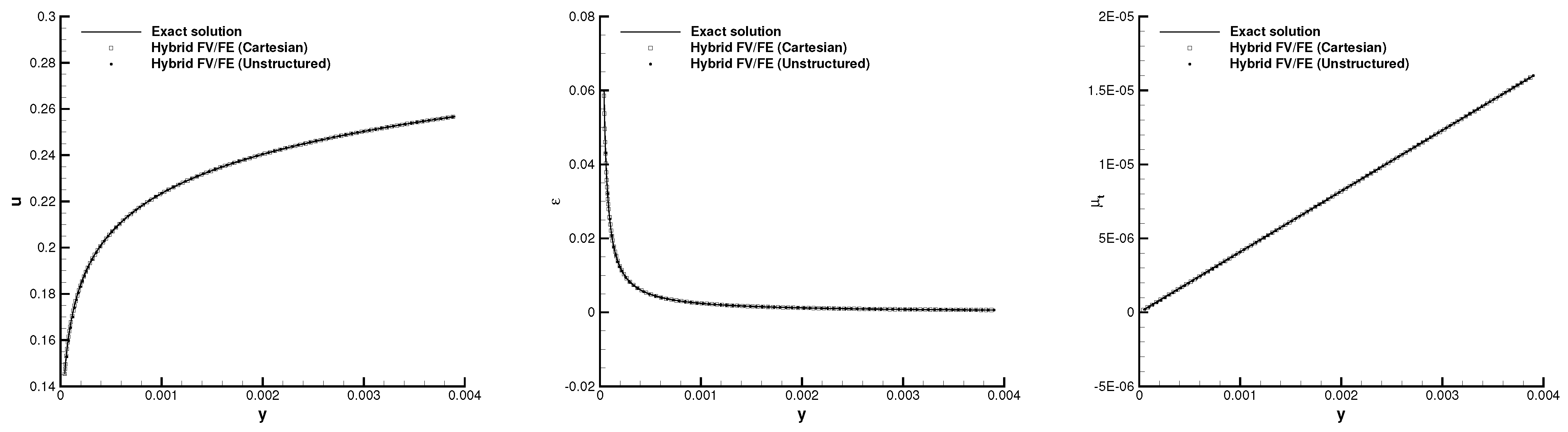
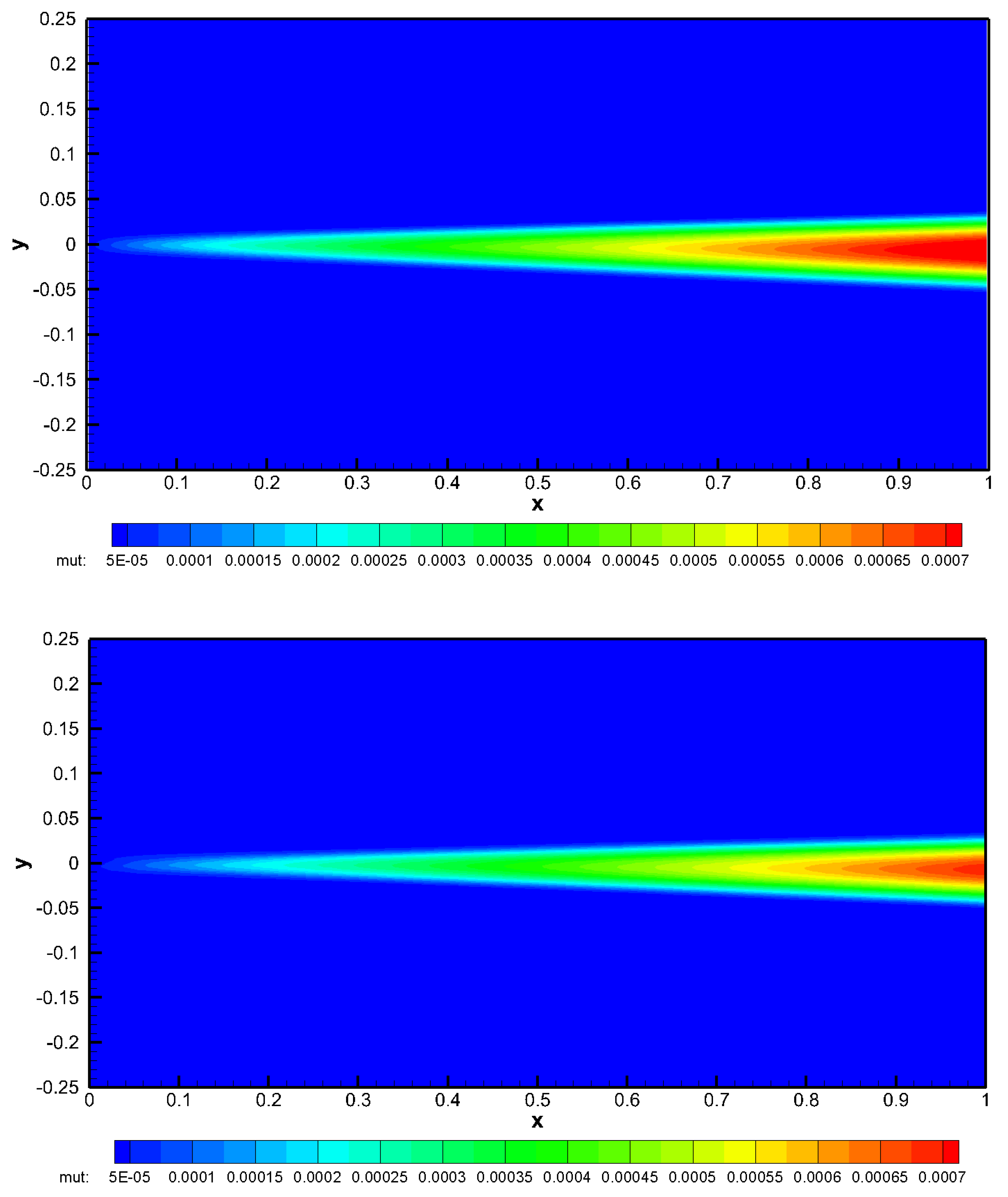
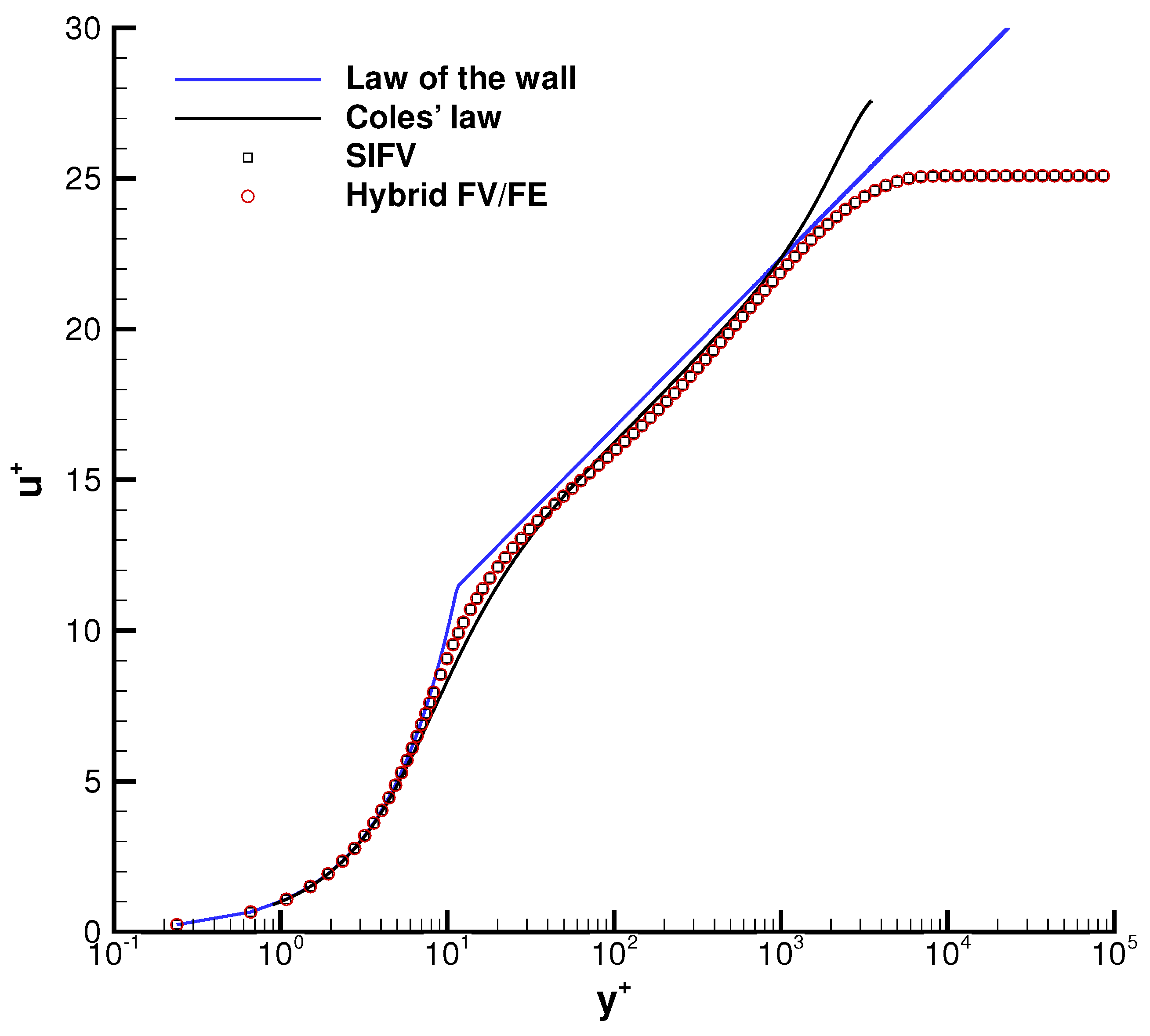
Table 1.
Description of the meshes and time steps used to perform the convergence analysis in triangular primal grids.
Table 1.
Description of the meshes and time steps used to perform the convergence analysis in triangular primal grids.
| Mesh | Elements | Vertices | Dual Elements | |
|---|---|---|---|---|
| 512 | 289 | 800 | ||
| 2048 | 1089 | 3136 | ||
| 8192 | 4225 | 12,416 | ||
| 32,768 | 16,641 | 49,408 | ||
| 131,072 | 66,049 | 202,687 | ||
| 524,288 | 263,169 | 787,456 | ||
| 2,097,152 | 1,050,625 | 3,171,158 |
Table 2.
Spatial error norms and convergence rates for the MMS test obtained at time using the hybrid FV/FE method for Cartesian grids.
Table 2.
Spatial error norms and convergence rates for the MMS test obtained at time using the hybrid FV/FE method for Cartesian grids.
| 20 | ||||
| 40 | ||||
| 80 | ||||
| 160 |
Table 3.
Spatial error norms and convergence rates for the MMS test obtained at time using the hybrid FV/FE method for unstructured grids.
Table 3.
Spatial error norms and convergence rates for the MMS test obtained at time using the hybrid FV/FE method for unstructured grids.
| Mesh | ||||
|---|---|---|---|---|
| M1 | ||||
| M2 | ||||
| M3 | ||||
| M4 | ||||
| M5 | ||||
| M6 | ||||
| M7 |
Table 4.
Spatial error norms obtained for the turbulent Couette flow at time using the hybrid FV/FE method for Cartesian grids and for unstructured simplex meshes.
Table 4.
Spatial error norms obtained for the turbulent Couette flow at time using the hybrid FV/FE method for Cartesian grids and for unstructured simplex meshes.
| Hybrid FV/FE Scheme on Cartesian Grid | ||||
|---|---|---|---|---|
| Single precision | ||||
| Double precision | ||||
| Quadruple precision | ||||
| Hybrid FV/FE Scheme on Unstructured Triangular Mesh | ||||
| Single precision | ||||
| Double precision | ||||
| Quadruple precision | ||||
Publisher’s Note: MDPI stays neutral with regard to jurisdictional claims in published maps and institutional affiliations. |
© 2021 by the authors. Licensee MDPI, Basel, Switzerland. This article is an open access article distributed under the terms and conditions of the Creative Commons Attribution (CC BY) license (https://creativecommons.org/licenses/by/4.0/).
Share and Cite
MDPI and ACS Style
Busto, S.; Dumbser, M.; Río-Martín, L. Staggered Semi-Implicit Hybrid Finite Volume/Finite Element Schemes for Turbulent and Non-Newtonian Flows. Mathematics 2021, 9, 2972. https://0-doi-org.brum.beds.ac.uk/10.3390/math9222972
AMA Style
Busto S, Dumbser M, Río-Martín L. Staggered Semi-Implicit Hybrid Finite Volume/Finite Element Schemes for Turbulent and Non-Newtonian Flows. Mathematics. 2021; 9(22):2972. https://0-doi-org.brum.beds.ac.uk/10.3390/math9222972
Chicago/Turabian StyleBusto, Saray, Michael Dumbser, and Laura Río-Martín. 2021. "Staggered Semi-Implicit Hybrid Finite Volume/Finite Element Schemes for Turbulent and Non-Newtonian Flows" Mathematics 9, no. 22: 2972. https://0-doi-org.brum.beds.ac.uk/10.3390/math9222972
Note that from the first issue of 2016, this journal uses article numbers instead of page numbers. See further details here.