A Scheduling Approach for the Combination Scheme and Train Timetable of a Heavy-Haul Railway

Abstract

Heavy-haul railway transport is a critical mode of regional bulk cargo transport. It dramatically improves the freight transport capacity of railway lines by combining several unit trains into one combined train. In order to improve the efficiency of the heavy-haul transport system and reduce the transportation cost, a critical problem involves arranging the combination scheme in the combination station (CBS) and scheduling the train timetable along the trains’ journey. With this consideration, this paper establishes two integer programming models in stages involving the train service plan problem (TSPP) model and train timetabling problem (TTP) model. The TSPP model aims to obtain a train service plan according to the freight demands by minimizing the operation cost. Based on the train service plan, the TTP model is to simultaneously schedule the combination scheme and train timetable, considering the utilization optimal for the CBS. Then, an effective hybrid genetic algorithm (HGA) is designed to solve the model and obtain the combination scheme and train timetable. Finally, some experiments are implemented to illustrate the feasibility of the proposed approaches and demonstrate the effectiveness of the HGA.

1. Introduction

1.1. Background

Heavy-haul railways have been the backbone of the coal transportation system because of their high capacity [1] and high efficiency for a long time. With the continuous growth of freight volume, the number of trains in the heavy-haul railway system keeps increasing, which brings great difficulties to the transportation plans’ scheduling and operation management in both stations and trunk lines. Therefore, one of the emergency issues that railway operators are concerned about is how to schedule transportation plans to reduce operating costs while ensuring transportation demand.

After North American railways took the lead in adopting heavy-haul railway transportation in the 1950s, this transportation mode quickly adapted to the needs of bulk cargo transport such as for coal, ore, etc., and developed rapidly in the world. The United States, Canada, Russia, Brazil, China, South Africa, Australia, Sweden, and more than ten other countries have carried out heavy-haul railway transportation. The heavy-haul railway transportation mode dramatically improves the freight transport capacity of railway lines by combining several unit trains into one combined train. Taking China as an example, the supply and demand for coal are extremely uneven geographically. The eastern region of China has been economically developed and its industrial production has a great need for coal resources. However, coal resources are mainly distributed in the western region [2]. Under this particular distribution pattern of natural resources, developing a heavy-haul railway can effectively guarantee coal supply and transportation.

With the rapid growth of the demand for heavy-haul transportation, railway operators have proposed a series of measures to guarantee the transport capacity of the heavy-haul railway, including increasing the load of combined trains, running different types of combined trains, and reducing the headway of adjacent trains. Under the condition that railway infrastructure cannot be revolutionarily upgraded, the flexible organization of several types of combined trains is one of the most effective ways for railway operators to satisfy the freight demand at a lower cost. From a transportation system-wide perspective, a reasonable heavy-haul railway transportation plan should meet the transportation demand, reduce the station operation workload, and reduce the operation cost.

A complete heavy-haul railway transportation plan consists of several sub-plans. It includes the train service plan, train combination scheme, train timetable, locomotive circulation scheme, empty train return scheme, decomposition scheme, etc. The heavy-haul railway operators are involved in various steps of the decision-making process to obtain a complete heavy-haul railway transportation plan. Six main stages in the decision-making process of the heavy-haul railway transportation plan are listed below.

(1) Collect the transport demand. The railway operators collect the buyers’ transport requirements, including the number and the destination of the required bulk goods.

(2) Schedule the train service plan. Determine the number and type of heavy-haul trains running between each station pair under the given unloading station requirements and loading station capacity conditions.

(3) Schedule the train combination scheme. In a heavy-haul railway system, the unit trains must be combined at a combination station (CBS) to run towards the unloading stations. Therefore, a detailed combination scheme should be arranged for the unit trains in the CBS.

(4) Schedule the train timetable. Based on the train combination scheme, determine all trains’ arrival and departure times at each station.

(5) Schedule the locomotive circulation scheme and train maintenance scheme. Heavy-haul trains generally require multi-locomotive traction. Set up the trains’ locomotive circulation and train maintenance schemes according to the preset locomotive routing and maintenance procedures.

(6) Schedule the empty train return scheme and the decomposition scheme. After the combined trains’ unloading at the unloading stations, the empty trains must return to the CBS for decomposition operations and return to the loading stations.

This paper focuses on developing a joint scheduling approach to schedule the (2)–(4) stages listed above. The decision-making process of the (2)–(4) stages is a complex process guided by transport demand. Figure 1 illustrates the relations between the stages in the decision-making process. It starts by collecting the loading capacity of each loading station and the requests for each unloading station’s demand. Then, heavy-haul railway operators need to generate executable combination schemes and train timetables based on the collected information according to the actual situation of the heavy-haul railway. The decision-making process at these stages needs to comprehensively consider all kinds of information of the heavy-haul railway transportation system and reflect it into the transportation plan.

1.2. Literature Review

In the early stage, heavy-haul transportation was mainly carried out to relieve the tight transportation capacity on busy trunk lines. Thus, the research focused mainly on freight transportation organization from a macro perspective. Fan [3] took the selectivity of the traffic flow path, the line capacity, and the unloading area of the heavy-haul railway into the optimization process and constructed an optional optimization model for the loading area. Yang [4] considered the logical matching relationship for the weight, speed, and density of heavy-haul railways to be a critical factor in freight railways and the matching relations of these three elements should be assured according to the country economy, society needs, and routes’ essential condition. Ma [5] discussed the external and internal factors that affect heavy-haul railways. The external factors include economic development, transportation price, and production factor price. In contrast, the internal factors include loading capacity, station capacity, unloading capacity, and maintenance capacity. Sun [6] analyzed the traffic capacity of coal transportation in the Baotou-Shenmu Railway and suggested strengthening the carrying capacity according to the present and further freight volume. Zhou [7] put forward strategies to improve the heavy-haul railway carrying capacity of the Baotou-Shenmu Railway in stations, improve train transportation efficiency and traction quality, and optimize the heavy-haul transportation organization plan, among other strategies as well.

With the increase of the freight volume of the heavy-haul railway, scholars have begun discussing the organization of the railcar flow in heavy-haul transport systems, focusing mainly on the relationship between the demand of cargo and the handling capacity of the railway system. Xue [8] proposed a method calculating the coupling degree between the station stages plan and the given dynamic railcar flow. Wang [9] studied the heavy-haul train operation plan problem with a multi-objective programming model, taking the prescriptive transportation volume index, the capacity of the railway line, and the available locomotives as the constraints. Zhao [10] established an optimization model of railcar flow organization in the loading area of the heavy-haul railway to minimize the combination time consumption and to maximize the flow of the heavy-haul railway. Then, he solved the model with the minimum cost and maximum flow algorithm. Tang [11] also built a minimum cost maximum flow model, of which the optimization goal is to maximize the operation time saved by direct transportation. Wang [12] focused on the cost of cargo flow in transit and established a 0–1 non-linear programming model with the objective of achieving the least cost. Jing [13] established the optimization model of direct flow in the loading area with the least operation time and lowest running consumption.

The increasing freight volume also increased the workload of stations in the heavy-haul railway systems. However, the manual approaches are still widely used in the actual railway operation, which are time-consuming and highly rely on the experience of the design managers [14]. Thus, scholars also paid attention to the organizational optimization of heavy-haul railway stations. The station technical operation is an essential part of the heavy-haul railway transportation organization. The stations of heavy-haul railways can be divided into four types: loading stations, CBS, unloading stations, and intermediate stations [15], which mainly handle the loading, unloading, combined, and decomposed operations. Among these types, the CBS is primarily responsible for the combined operations of heavy trains based on the combination scheme [16]. Hence, it is an important node of the heavy-haul railway at the macro level. After realizing the critical role of station technical schemes in the operation and the management of heavy-haul railway systems, scholars began to focus on the research about the CBS.

Along this line, Wei [17] studied the influence of turnout selection on the passing capacity of heavy-haul railway stations, the additional start or stop time of trains, the period of the train timetable, and the headway of tracks. Ye [18] analyzed the reasons for the station’s passing capacity based on the operation of 20,000 tons of combined trains in Hudong Station. He put forward an optimized organization plan to ensure heavy-haul trains’ safe transportation in Hudong Station. Liang [19] calculated the time that the trains occupied the station track by analyzing the operation process of the combined trains in the CBS and checked the number of the station arrival–departure tracks setting in Hudong Station. Tang [11] studied the operation organization of Hudong Station on the Daqin Railway and made an in-depth analysis of the organization mode of train queuing. In the cargo flow organization model established by him, the optimization goal is to maximize the adaptation time saved by direct transportation. Under constraints of the combination regulations, train’s weight, the latest permissible time for the combination of the departure trains, etc., the non-linear 0–1 programming model was established by Han [20] with the objective of the minimum station dwell time and decomposition time of the heavy-haul train at CBS. Ma [21] constructed the linear 0–1 programming model and quadratic 0–1 programming model, setting the utilization equilibrium and the track’s selection tendency as the objective functions.

The heavy-haul railway transport is a particular pattern of railway freight transport, which is different from the general passenger and freight railway transport. From the whole network scale perspective, the heavy-haul railway is a radial tree-shaped network with strong system independence rather than a large-scale network structure. From the view of station operation in the technical station, the heavy-haul trains need to be combined or decomposed in the CBS with unit trains as the minimum unit, which is similar to the freight train’s marshaling. The scheduling of the combined scheme in the CBS of the heavy-haul railway can be regarded as a special case of the train formation problem (TFP). The TFP determines the routing and frequency of trains and assigns the demands to trains [22].

The TFP has received research attention from a mathematical point of view. Therefore, the transportation organization of heavy-haul railway stations can also learn from some research studies based on marshaling yards. For example, a neural network is examined for obtaining good solutions in short time periods for the TFP by Martinelli [23]. Xiao [14] established the comprehensive optimization model of the train formulation plan using both the single-block trains and two-block trains, aimed at the minimization of the total car–hour consumption at all yards. As for a discrete deterministic-controlled system that simulates the operation of the flat yard, Kozachenko [24] obtained a mathematical statement of the problem of choosing the optimal order of multi-group train formation. Lin [25] built a bi-level linear integer model to solve the train service network problem of the Chinese railway system. Later, he [26] presented the formulation of a train formation problem in rail loading stations from a systematic perspective. Yaghini [27] proposed a hybrid algorithm of the simplex method and simulated annealing for the train formation problem. Murali [28] presented a decision tool to aid train planners to obtain good quality routes and schedules quickly for short-time horizons. Lazarev [29] provided the integer linear programming statement to form trains and define both their routes and schedules by minimizing the total weighted delivery time of all orders.

There are mainly two differences between heavy-haul railway transport and general freight railway transport. Firstly, at the beginning of the transport, the loading stations need to load a particular length of unit trains without specifying the destination of each railcar. In contrast, in the general freight railway system, different railcars have specific destinations, thus railway operators need to combine the railcars with similar destinations into a train. Secondly, at the end of the transport, considering that the unloading stations in the heavy-haul railway have a large unloading capacity, the railway operators transport the combined trains into specific unloading stations directly.

To our knowledge, however, there are few demand-oriented scheduling approaches of heavy-haul railway transportation plans. This paper is particularly interested in proposing a new approach to simultaneously schedule the combination scheme and heavy-haul train timetable on a heavy-haul railway considering the demand of the unloading area.

The rest of this paper is organized as follows. Section 2 introduces the general form of a heavy-haul railway network and the operation process of trains in the heavy-haul transport system. We also explain several terms of the heavy-haul transport system. Section 3 describes the problem and proposes two optimization models to solve the heavy-haul railway’s combination scheme and train timetable. Section 4 designs a hybrid algorithm based on the genetic algorithm framework to solve the proposed model. In Section 5, a small case and a real-world case are solved by the proposed approach to prove the method’s effectiveness. Section 6 presents some conclusions.

2. Conceptual Illustration

This section will introduce the composition of a heavy-haul railway and the operation process of trains in the railway system.

2.1. Composition of the Heavy-Haul Railway

The heavy-haul railway usually connects the railway to the production side and the demand side of bulk cargo like a corridor. Thus, it is also called the heavy-haul railway corridor. It has the characteristics of high independence and large carrying capacity. The heavy-haul railway corridor is usually a special freight railway line used to transport a particular type of bulk cargo. This kind of heavy-haul railway generally transports a single type of cargo and operates massive railcars’ flow every day.

Figure 2 is a simplified schematic diagram of a heavy-haul railway. As shown in the figure, a typical heavy-haul railway can be divided into three parts: loading area, transport area, and unloading area.

• Loading area

The loading area contains two types of technical stations. One is the loading station, which is the place where the unit trains are loaded. The loading stations in the loading area mainly connect to the trunk line through branch railway lines. Empty railcars are loaded at loading stations and become heavy unit trains (in the following text, we call it unit trains). Part of the heavy unit trains also directly turn into the heavy-haul railway through the boundary (the boundary connects the heavy-haul railway to other railway lines). Another technical station is the CBS, the most critical technical station in the heavy-haul railway system. The unit trains would be sent here for combined operation. The unit trains are assembled here and combined into combined trains for the unloading area.

2.

Transport area

The transport area is the trunk line between the CBS and the unloading area. According to the train timetable, the combined trains run on the trunk line to transport the bulk cargo to the unloading area.

3.

Unloading area

The unloading area is the end of a heavy-haul railway. Here, the buyer submits the demand and hands over the bulk cargo. Part of the branch line in the unloading area is not directly connected to the unloading station but is a boundary connecting other railway lines. The combined trains will arrive at the unloading stations to unload the bulk cargo or to be transferred from the boundary to other places. The combined trains become empty trains after unloading at the unloading station.

For the sake of simplification, this paper considers that all unit trains will be combined in the CBS. However, there were also a number of direct trains on the heavy-haul railways that only need a simple inspection operation at the CBS. As running trains directly connect to the destination, it is helpful to reduce the workload of the CBS [30], and some loading stations load and send specific types of combined trains. These trains do not need combined operation when through the CBS. For this scenario, when these direct trains run between the loading area and the CBS, we regard them as unit trains. When they run between the CBS and unloading area, we regard them as combined trains. We also treat the inspection operation of direct trains in CBS as a combined operation.

2.2. Operating Process of Trains

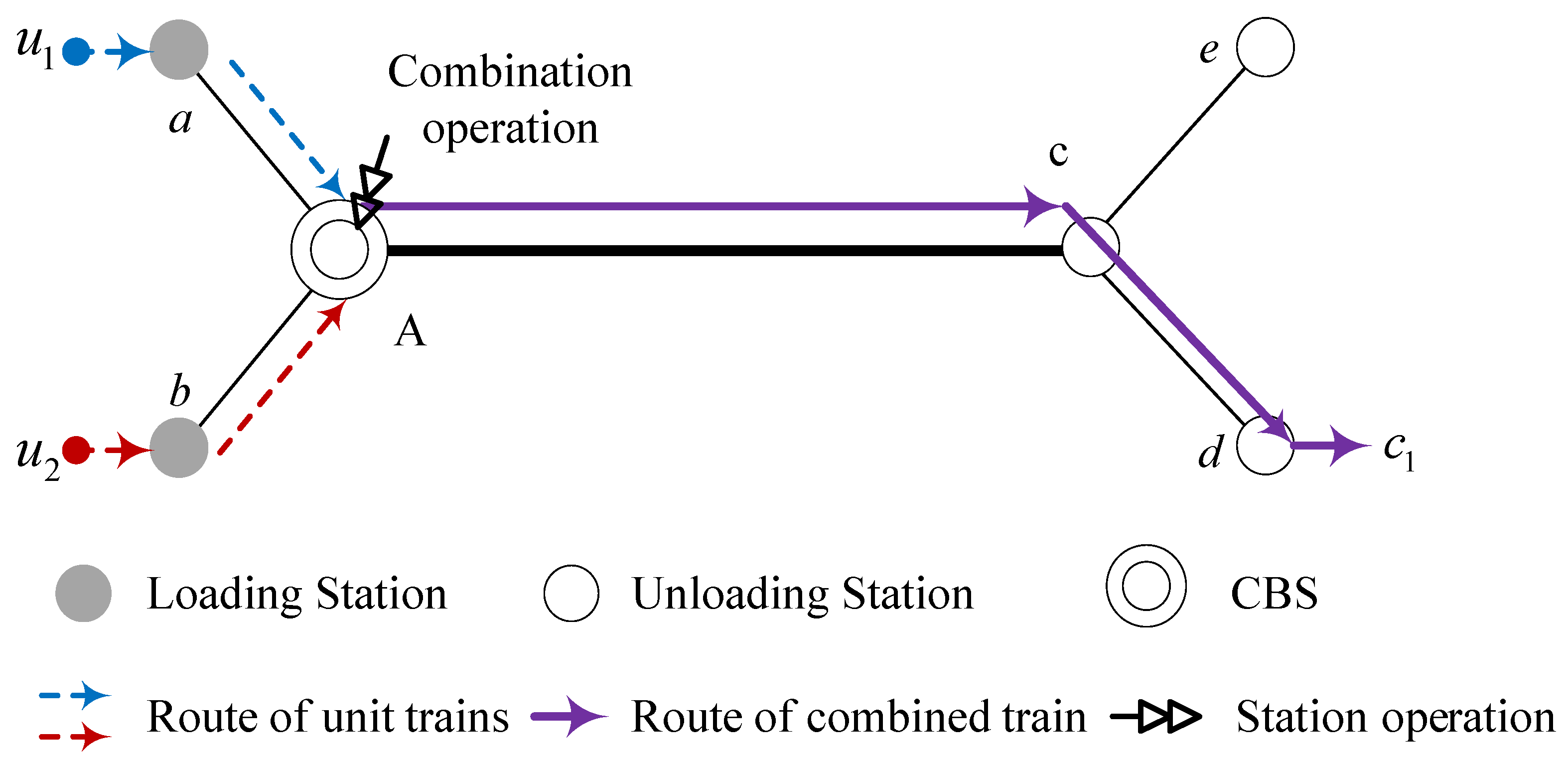
In order to intuitively introduce the operational process of unit trains and the combined trains in a heavy-haul railway system, an illustration of a small heavy-haul railway network is given below.

As shown in Figure 3, A is the CBS in a small-scale heavy-haul railway network. The unloading station d requires 10 kt of coal. Therefore, two unit trains with 5 kt loads are sent to the unloading station d from both loading station a and loading station b. Unit train $u_1$ (blue dotted arcs) departs from loading station a, and unit train $u_2$ (red dotted arcs) departs from loading station b. At the CBS A, $u_1$ and $u_2$ are combined into a combined train $c_1$ (purple arcs) with a 10 kt total load.

When we extend this physical railway network on the time axis, we can find more temporal details from the time–geography perspective. As shown in Figure 4, the vertical axis corresponds to time and we discretize consecutive periods into small increments. The benefit of adopting a space–time network framework is to precisely capture the temporal and spatial interaction of the transportation system [31]. In this way, we can intuitively understand the moving trajectory of the trains in the heavy-haul railway. The process of train operation in the heavy-haul railway can be divided into two types: travel in the section and station technical operation.

4.

Travel in the section

The straight arcs in Figure 4 are the space–time trajectories of the trains. They show the spatial and temporal displacement of the train in the sections. The start of the straight arcs means the section’s origin station and the train’s departure time. The end of the straight arcs means the section’s destination station and the train’s arrival time. Thus, the duration of the straight arcs reflects the train’s running time in the section. The running time of the trains in a section is generally constant because the trains do not need to perform additional operations in the section.

5.

Station technical operation

Train station operations in the heavy-haul railway include loading operations at the loading station, unloading operations at the unloading station, and technical operations at the CBS. After arriving at the CBS, the unit train needs to connect other pre-designated unit trains as a combined train. The whole combined operation includes the process of arriving, changing locomotives, connecting trains, and train inspection. A combined operation usually takes more than 2 h. However, the direct trains only need to carry out the train inspection at the CBS rather than participate in the combined operation. Here, we treat train inspection as a special combination of operations. All heavy-haul trains need to finish the technical operation at the CBS before they can be dispatched to the trunk line.

As shown in Figure 4, the duration of a unit train’s staying in the CBS is the dwell time from the unit train’s arrival to its departure after combining into a combined train, including the headway and all combined operation times. Obviously, the longer unit trains stay in the CBS, the longer cargo will be in transit, increasing delivery time. At the same time, the unit trains occupy the resources such as tracks in the CBS, which will reduce the station’s utilization. Therefore, in actual operation, we hope to reduce the total dwell time of unit trains in the CBS as much as possible so as to improve the efficiency of CBS operations and to reduce the delivery time of cargo.

The technical operations of the CBS are based on a combination scheme. The combination scheme will specify when the unit trains arrive at the CBS, will assign the specific constituent unit trains for the combined train, and will specify when the combined train will be dispatched from the CBS. The formulation of the combination scheme determines the total dwell time of the unit trains in the CBS. Therefore, optimizing the combination scheme is the key point to improve the efficiency of the heavy-haul transport system.

2.3. Framework

This paper proposes a new methodology using a hybrid genetic algorithm to simultaneously account for cargo transportation demand and station technical operation to optimize both train combination scheme and timetable. Thus, the heavy-haul transport system can meet the transportation service at a lower cost. The framework of our proposed methodology is illustrated in Figure 5.

To simplify the problem, we divide the heavy-haul railway transportation plan problem into two stages. In the first stage, the heavy-haul train service plan is designed. The cargo demand and heavy-haul railway’s operating conditions determine the number of each type of heavily loaded train between different stations. The second stage is to schedule an appropriate combination scheme and train timetable for the heavy-haul train service plan generated in the first stage.

3. Optimization Model

To provide high-performance transportation services, railway operators need to optimize the heavy-haul railway transportation plan based on the required demand. In this section, we describe the train service plan problem (TSPP) and the train timetabling problem (TTP).

Table 1. Sets, indices, and parameters.

Symbol	Definition
$T$	The set of combined trains and unit trains
$T^{com}$	The set of combined trains, $T^{com}\in T$
$T^{uni}$	The set of unit trains, $T^{uni}\in T$
$S$	The set of stations
$V$	The set of sections
$K$	The set of combined train types
$U$	The set of unit train types
$p$	The index of combined trains, $p\in T^{com}$
$q$	The index of unit trains, $q\in T^{uni}$
$i$, $j$	The index of stations, $i,j\in S$
$s_z$	The label of the CBS, $s_z\in S$
$S_{loa}$	The set of loading stations, $S_{loa}\in S$
$S_{unl}$	The set of unloading stations, $S_{unl}\in S$
$\left(i,j\right)$	The label of the section that connects station $i$ and station $j$, $\left(i,j\right)\in V$
$k$	The index of combined train types, $k\in K$
$u$	The index of unit train types, $u\in U$
$p\left(i,j\right)$	$p\left(i,j\right)\in \left\{0,1\right\}$; if combined train $p$, choose the section $\left(i,j\right)$, $p\left(i,j\right)=1$, otherwise $p\left(i,j\right)=0$
$q\left(i,j\right)$	$q\left(i,j\right)\in \left\{0,1\right\}$; if unit train $q$, choose the section $\left(i,j\right)$, $q\left(i,j\right)=1$, otherwise $q\left(i,j\right)=0$
$p_k$	$p_k\in \left\{0,1\right\}$; if the type of combined train is $k$, $p_k=1$, otherwise $p_k=0$
$I_k$	The minimum headway of the combined train when its type is $k$
$I_u$	The minimum headway of the unit train when its type is $u$
$q_u$	$q_u\in \left\{0,1\right\}$; if the type of unit train $q$ is $u$, $q_u=1$, otherwise $q_u=0$
${\phi }_{k,u}$	The number of u-type unit trains required to combine a k-type combined train, ${\phi }_{k,u}\in \mathbb{Z}$
$t_k^{tec}$	The total dwell time of the k-type combined train in the CBS
$r\left(i,j\right)$	The running time of trains running on the section $\left(i,j\right)$
$w_u$	The number of railcars in a u-type unit train
$l_i^{cap}$	The unloading capacity of the unloading station $i$
$l_i^{dem}$	The demand for unloading station $i$
${\mu }_k$	The cycle length of train turn-around
$M$	A big enough positive number
$c_k$	The cost of running a k-type combined train
$\lambda$	The section capacity utilization
$t_{\lambda }$	Longest service time of the railway line
$D^{start},D^{end}$	The allowable starting and ending time for combined trains
$A^{start},A^{end}$	The allowable starting and ending time for unit trains

lists the sets, indices, and parameters used in this paper.

3.1. Train Service Plan Problem (TSPP) Model

The heavy-haul railway train service plan should include the following parts: the type and quantity of the unit trains departing from each loading station, and the type and quantity of the combined trains arriving at each unloading station.

In a heavy-haul railway system, the combined trains take on the transport between the CBS and unloading stations. The combined trains require different operation times and human resources, and cause different track wear due to their different total loads. Thus, the operating cost of the different types of the combined trains is different. However, the heavy-haul railway train service plan involves a key criterion, which is railway operators’ profitability [32]. To this end, we introduce an optimization model that intends to minimize the total cost requirements. The problem also aims to determine the number of $u$-type unit trains departing from loading station $i$ to the CBS, which can be defined by variable $y_i^u$, and to determine the number of $k$-type combined trains departing from the CBS to unloading station $j$, which can be defined by variable $x_j^k$.

Table 2. Decision variables for the TSPP model.

Symbol	Definition
$y_i^u$	The number of u-type unit trains departing from loading station i to the CBS, $i\in S_{loa}$
$x_j^k$	The number of k-type combined trains departing from the CBS to unloading station $j$, $j\in S_{unl}$

lists the two types of variables used in this model.

• Problem statement

A heavy-haul railway system has several loading and unloading stations. Given the loading stations’ capacity, the unloading stations’ demand, and the unloading capacity. Find a train service plan to meet the cargo demand to make the total operation cost minimal.

2.

Objective function

The objective function is to minimize the operating costs of the heavy-haul railway. $c_k$ denotes the cost of running a $k$-type combined train. The parameter $c_k$ can be calibrated by the experience of the railway operator.

$$\min z={\displaystyle \sum _{j\in S_{unl}}{\displaystyle \sum _k{c}_k{x}_j^k}}$$

(1)

3.

Demand constraints

Constraint (2) ensures that the cargo that can be transported by the combined trains, arriving at the unloading station within one day, shall meet the demand for the cargo at the unloading station.

$${\displaystyle \sum _k{\displaystyle \sum _u{x}_{{}_j}^k{\phi }_{k,u}{w}_u}}\ge l_j^{dem},\forall j\in S_{unl}$$

(2)

4.

Unloading capacity constraints

Due to the limited unloading capacity of each unloading station, the quantity of cargo to be carried by the combined trains arriving at each unloading station shall be less than the daily unloading capacity of the unloading station.

$${\displaystyle \sum _k{\displaystyle \sum _u{x}_j^k{\phi }_{k,u}{w}_u}}\le l_j^{cap},\forall j\in S_{unl}$$

(3)

5.

Loading capacity constraints

Due to the limited loading capacity of each loading station, the number of unit trains departing from each loading station shall be less than the daily loading capacity of the loading station.

$${\displaystyle \sum _u{y}_i^u{w}_u}\le l_i^{cap},\forall i\in S_{loa}$$

(4)

6.

Section carrying capacity constraints

In a heavy-haul railway’s trunk line and branch lines, the headway between any two adjacent trains should be greater than the minimum headway. As a result, the number of trains going through the heavy-haul railway every day is limited. Therefore, the number of unit trains or combined trains passing through any section should be less than the section carrying capacity.

$${\displaystyle \sum _j{\displaystyle \sum _k{I}_k{y}_j^k}}\le t_{\lambda }$$

(5)

7.

Flow balance constraint for the CBS

The unit trains arriving at the CBS are combined into the combined trains and sent into the trunk line. The CBS cannot be used as a storage place for trains, thus the number of railcars arriving at the CBS is equal to the railcars departing from it.

$${\displaystyle \sum _{j\in S_{unl}}{\displaystyle \sum _k{x}_j^k{\phi }_{k,u}}}={\displaystyle \sum _{i\in S_{loa}}{y}_i^u},\forall u\in U$$

(6)

3.2. Train Timetabling Problem (TTP) Model

In our approach, the result of the TSPP model provides input parameters related to the train timetable. Since we already know the number of different types of unit trains and combined trains that need to be operated in the heavy-haul railway, we need to further develop appropriate schedules for these trains.

The goal of the TTP model is to schedule the trains to minimize the total dwell time in the CBS. The model also aims to determine the combination relationship between the unit trains and combined trains, which can be defined by variable ${\theta }_{p,q}$. Here, we use two groups of decision variables. The unit train schedule variable $d_q\left(i,j\right)$ and $a_q\left(i,j\right)$ denote the departure time and arrival time of unit train $q$ in station $i$ and station $j$. The combined train schedule variable $d_p\left(i,j\right)$ and $a_p\left(i,j\right)$ denote the departure time and the arrival time of combined train $p$ in station $i$ and station $j$.

Table 3. Decision variables for the TTP model.

Symbol	Definition
$a_p\left(i,j\right)$	The arrival time of combined train $p$ arriving at station $j$ from section $\left(i,j\right)$
$a_q\left(i,j\right)$	The arrival time of unit train $q$ arriving at station $j$ from section $\left(i,j\right)$
$d_p\left(i,j\right)$	The departure time of combined train $p$ departing from station $i$ to section $\left(i,j\right)$
$d_q\left(i,j\right)$	The departure time of unit train $q$ departing from station $i$ to section $\left(i,j\right)$
${\theta }_{p,q}$	Unit train assignment variable (if the combined train $p$ is combined by unit train $q$, ${\theta }_{p,q}=1$; otherwise, ${\theta }_{p,q}=0$)

lists the variables used in this model.

• Problem statement

Given the number and type of unit trains and combined trains that need to be operated in the heavy-haul railway system, determine the trains’ combination scheme in the CBS and the train timetable of each station to make the total dwell time minimal.

2.

Objective function

The objective function is to minimize the total dwell time of the trains in the CBS. The function ${\displaystyle \sum _p{d}_p\left(i,j\right){\theta }_{p,q}}$ denotes the departure time of combined train $p$. Additionally, suppose the combined train $p$ is composed of unit train $q$. The dwell time of unit train $q$ in the CBS can be calculated by the function ${\displaystyle \sum _p{d}_p\left(i,j\right){\theta }_{p,q}}-a_q\left(i,j\right)$. Thus, the total dwell time of unit trains in the CBS can be expressed by (7).

$$\min z_2={\displaystyle \sum _q\left[{\displaystyle \sum _p{d}_p\left(s_z,j\right){\theta }_{p,q}}-a_q\left(i,s_z\right)\right]}, \forall p\in T^{com},\forall q\in T^{uni}$$

(7)

3.

Minimum station operating time constraints

The dwell time of trains must be longer than its minimum station operating time to ensure the necessary combined operation before departure. Constraint (8) guarantees the minimum station operating time of combined train $q$ in the CBS. $M$ is a big enough positive number. If combined train $p$ is not composed of unit train $q$, the right-hand side of the inequality is equal to a big enough negative number, thus the inequality is always true. If combined train $p$ is composed of unit train $q$, the right-hand side of the inequality is equal to the minimum station operating time.

$$d_p\left(s_z,j\right)-a_q\left(i,s_z\right)\ge {\theta }_{p,q}{t}^{tec}+\left({\theta }_{p,q}-1\right)M,\forall p\in T^{com},\forall q\in T^{uni}$$

(8)

4.

Marshalling constraints

Each type of combined train has a prescribed rule of marshaling which specifies the type and number of the component unit trains. For example, a 15 kt combined train is composed of three 5 kt unit trains and a 10 kt combined train is composed of two 5 kt unit trains. It is worth noting that a 10 kt unit train can be sent into the trunk line directly without marshaling. For the sake of description in the model, we describe it as a 10 kt combined train composed of a 10 kt unit train in this scenario.

$${\displaystyle \sum _q{\theta }_{p,q}{q}_u={\displaystyle \sum _k{p}_k{\phi }_{k,u}}},\forall p\in P,\forall u\in U$$

(9)

5.

Running time constraints

$r\left(i,j\right)$ denotes the running time of trains in section $\left(i,j\right)$. Equation constraints (10) and (11) enforce the rule that the running time of combined trains and unit trains should equal to $r\left(i,j\right)$ if $\left(i,j\right)$ is in its route.

$$a_p\left(i,j\right)-d_p\left(i,j\right)=r\left(i,j\right)p\left(i,j\right),\forall \left(i,j\right)\in V,\forall p\in T^{com}$$

(10)

$$a_q\left(i,j\right)-d_q\left(i,j\right)=r\left(i,j\right)q\left(i,j\right),\forall \left(i,j\right)\in V,\forall q\in T^{uni}$$

(11)

6.

Headway constraints

The headways of different types of trains are different. The function ${\displaystyle \sum _k{I}_k}{p}_k$ denotes the minimum headway of combined train $p$ and constraint (13) ensures that the interval between two adjacent combined trains in section $\left(i,j\right)$ must not be less than the minimum headway.

$$\left|a_{q\prime }\left(i,j\right)-a_q\left(i,j\right)\right|\ge {\displaystyle {\sum }_u{q}_u{I}_u},\forall q,q\prime \in T^{uni}$$

(12)

$$\left|a_{p\prime }\left(i,j\right)-a_p\left(i,j\right)\right|\ge {\displaystyle {\sum }_k{p}_k{I}_k},\forall p,p\prime \in T^{com}$$

(13)

7.

Operating period constraint

Both combined trains and unit trains must be operated within the permitted period.

$$a_q\left(i,s_z\right)\in \left[A^{start},A^{end}\right],\forall q\in T^{uni}$$

(14)

$$d_p\left(s_z,j\right)\in \left[A^{start},A^{end}\right],\forall p\in T^{com}$$

(15)

4. Hybrid Genetic Algorithm

To solve the TSPP model and TTP model for a heavy-haul railway system, we propose the following solution approach by solving the TSPP model using commercial solver GUROBI and solving the TTP model using a hybrid genetic algorithm (HGA). In this section, we introduce the detailed solving process of the HGA.

The TTP model is the optimal integration of a heavy-haul railway combined scheme and train timetable. It is a difficult problem since both the train formation problem and the train timetabling problem are NP-hard problems [22,33,34]. Therefore, to solve the TTP model, we developed a genetic algorithm-based framework.

Genetic algorithms (GA), first proposed by Holland [35], are inspired by natural genetic and evolutionary mechanisms to find high-quality solutions for complex problems. The genetic algorithm constructs a fitness function according to the objective function of the problem. The fitness value may directly or indirectly represent a solution to the original problem. The algorithm performs evaluation, genetic calculation, and selection on a population composed of multiple solutions (each solution corresponds to a chromosome), and after multiple generations of reproduction, the individual with the best fitness is the optimal solution to the problem. A population contains multiple individuals and for each their chromosome includes one or several gene fragments. The GA includes the following steps [36]: (1) chromosome representations; (2) initial populations generate; (3) fitness function; (4) genetic operations (including crossover and mutation); (5) selection mechanisms; and (6) termination condition.

The GA is widely used in industrial engineering, artificial intelligence, automatic control, and other fields because of its great potential in solving complex optimization problems [37].

Specifically, the HGA to solve the TTP model is set up as explained below.

4.1. Representation Scheme

In this solution approach, we represent solutions indirectly by parameters that are later used to obtain a solution by a special decoding procedure. Each solution chromosome is made of two gene fragments.

Gene fragment Ⅰ: The first gene fragment represents the departure sequence of the combined trains departing from the CBS. It is made of $N_c$ genes, where $N_c$ is the number of the combined trains. After obtaining the type and number of trains that need to run between the CBS and each loading station or unloading station, we create a unique index for each train. The value of the jth gene of gene fragment Ⅰ represents the departure sequence of train j.

Gene fragment Ⅱ: The second gene fragment is a matrix to represent the connection relationship between the unit trains and combined trains. When the number of combined trains is $N_c$ and the number of unit trains is $N_u$ and a $N_u\times N_c$, a matrix can be built and we call it the combination matrix. The combination matrix is a 0–1 matrix. If the value of row i and column j is 1, that means combined train j is composed of unit train i.

Figure 6 depicts a small example. As shown in the figure, seven unit trains are assigned into four combined trains in the CBS. Four combined trains, namely $c_1$, $c_2$, $c_3$, and $c_4$, depart the CBS in the sequence as 2, 1, 3, and 4, respectively. Thus, the departure sequence can be represented by the vector $\left(2,1,3,4\right)$. For combined train $c_1$, it consists of unit trans $u_1$ and $u_2$. Thus, its corresponding row in the combination matrix should be $\left(1,0,0,1,0,0,0\right)$.

4.2. Initial Populations and Infeasible Solution Adjustment

The combination matrix is a gene fragment of a chromosome generated randomly by initialization or through crossover and mutation. It may not satisfy the constraints of train marshaling. Therefore, infeasible combination matrix adjustment strategies are designed for chromosomes to obtain an available connection relationship. The infeasible combination matrix adjustment process is illustrated in Algorithm 1.

Algorithm 1 Infeasible combination matrix adjustment

Step 1. Calculate the initial number and type of unit trains that are combined into a combined train.    Create set $C_{\mathrm{com}}$, calculate the current number of unit trains connected to the combined train $p$, and let $c_p$ denote it. Then, add $c_p$ to $C_{com}$.    Step 2. Adjust chromosomes so that each combined train consists of a specified number of unit trains.    For each combined train $p\in T^{com}$    If $c_p$ $>{\phi }_{k,u}$      Create index set $R_{p1}$      Find out all indices $r$ where ${\theta }_{p,r}=1$ and add $r$ to $R_{p1}$      Create subset $R_{p2}$      Randomly choose ${\phi }_{k,u}-c_p$ elements $r\prime$ in $R_{p1}$ and add $r\prime$ to $R_{p2}$      Let ${\theta }_{p,r\prime }=0$ for all $r\prime$ in $R_{p2}$    If $c_p$ $<{\phi }_{k,u}$      Create index set $R_{p1}$      Find out all indices $r$ where ${\theta }_{p,r}=0$ and add $r$ to $R_{p1}$      Create subset $R_{p2}$      Randomly choose $c_p-{\phi }_{k,u}$ elements $r\prime$ in $R_{p1}$ and add $r\prime$ to $R_{p2}$      Let ${\theta }_{p,r\prime }=1$ for all $r\prime$ in $R_{p2}$    Step 3. Calculate the current number and type of unit trains that are combined into a combined train.    Create set $C_{unit}$, calculate the current number of combined trains connected to unit train $q$, and let $c_q$ denote it. Then, add $c_q$ to $C_{unit}$.    Step 4. Adjust chromosomes so that each unit train can be combined into, at most, one combination train.    Create index set $R_{q0}$    Find out all indices $s$ where $c_q=0$ and add $s$ to $R_{q0}$    For each unit train $q\in T^{uni}$    If $c_q>1$      Create index set $R_{q1}$     Find out all indices $r$ where ${\theta }_{r,q}=1$ and add $r$ to $R_{q1}$     Create subset $R_{q2}$, $R_{q3}$     Randomly choose $c_q-1$ elements $r\prime$ in $R_{q1}$ and add $r\prime$ to $R_{q2}$     Randomly choose $c_q-1$ elements $s\prime$ in $R_{q0}-{\displaystyle \sum _{q=1}^{q-1}{R}_{q3}}$ and add $s\prime$ to $R_{q3}$     Let ${\theta }_{r\prime ,q}=0$ for all $r\prime$ in $R_{q2}$ and let ${\theta }_{r\prime ,s}=0$ for all $s\prime$ in $R_{q3}$

4.3. Decoding

The chromosomes are made of two gene fragments that represent the combined trains’ departure sequence and the connection relationship; thus, the chromosomes have to be decoded to derive the combination scheme and train timetable. The chromosome decoding process is divided into three main steps. First, we transform the two gene fragments of the chromosome into the operation sequence of the trains. Then, we use a linear program to determine the combination scheme of the unit trains and the combined trains in the CBS. Finally, we calculate the train timetable according to the combination scheme.

First of all, we determine the order of any two combined trains departing from the CBS according to gene fragment Ⅰ of the chromosome. Next, determine the order of any two unit trains arriving at the CBS according to gene fragment Ⅱ. Here, we introduce two parameters, namely $O^{com}(p,p\prime )$ and $O^{uni}(q,q\prime )$. $O^{com}(p,p\prime )$ denotes the departure order of combined trains $p$ and $p\prime$. When combined train $p$ departs from the CBS before combined train $p\prime$, then $O^{com}(p,p\prime )=1$; otherwise, $O^{com}(p,p\prime )=0$. $O^{uni}(q,q\prime )$ denotes the arrival order of unit trains $q$ and $q\prime$. When unit train $q$ arrives at the CBS before combined train $q\prime$, then $O^{com}(q,q\prime )=1$; otherwise, $O^{com}(q,q\prime )=0$.

The process of determining the value of the parameters $O^{com}(p,p\prime )$ and $O^{uni}(q,q\prime )$ is shown in Algorithm 2. The calculation process of determining the operation sequence of trains can be divided into two steps. In step 1, we roughly calculate all trains’ arrival and departure times in the COS according to the departure sequence in gene fragment Ⅰ and the connection relationship in gene fragment Ⅱ. Then, in step 2, we determine the departure order of any combined train pair by sequencing in gene fragment Ⅰ. Similarly, we compare the arrival times in step 1 to determine the arrival order of any unit train pair. As a result, we derive an assignment to $O^{com}$ and $O^{uni}$.

Algorithm 2 Determine the operation sequence of trains in the CBS

Input: Gene fragment Ⅰ $g1$, gene fragment Ⅱ$G2$   Output: $O^{com}$, $O^{uni}$   Step 1: Initialize the departure time of the combined trains and the arrival time of the unit trains according to gene fragments Ⅰ and Ⅱ.   Create set $D^{com}$ to denote the initialized departure time of the combined trains   Create set $A^{uni}$ to denote the initialized arrival time of the unit trains   For each combined train $p\in T^{com}$    If $g1(p)=1$     Let $d_p=0$ and add $d_p$ to $D^{com}$    Else     If $g1(p)=g1(p\prime )+1$     Let $d_p=d_{p\prime }+{\displaystyle {\sum }_k{I}_{k}p{\prime }_k}$ and add $d_p$ to $D^{com}$   For each unit train $q\in T^{uni}$    $u=0$    For each combined train $p\in T^{com}$     If $G2(p,q)=1$     Let $a_q=d_p-{\displaystyle {\sum }_k{p}_k{t}_k^{tec}}-I_{u}u$ and add $a_q$ to $A^{uni}$     $u=u+1$   Step 2: Determine departure order $O^{com}$ for any combination train pair and arrival order $O^{uni}$ for any unit train pair.   Create set $O^{com}$ of the combined train departure order   Create set $O^{uni}$ of the combined train arrival order   For each combined train $p\in T^{com}$    For each combined train $p\prime \in T^{com}$     If $g1(p)<g1(p\prime )$      Let $o_{p,p\prime }=1$ and add $o_{p,p\prime }$ to $O^{com}$     Else      Let $o_{p,p\prime }=0$ and add $o_{p,p\prime }$ to $O^{com}$   For each unit train $q\in T^{uni}$    For each combined train $q\prime \in T^{uni}$     If $a_q<a_{q\prime }$      Let $o_{q,q\prime }=1$ and add $o_{q,q\prime }$ to $O^{uni}$     Else      Let $o_{q,q\prime }=0$ and add $o_{q,q\prime }$ to $O^{uni}$

After the train operation sequence is determined, the solution space of the original problem is greatly reduced. Using parameters $O^{com}(p,p\prime )$, $O^{uni}(q,q\prime )$, and a large positive number M, we can rewrite the absolute value inequality in constraints (12) and (13). The operation time of the combined trains and unit trains in the CBS can be easily solved. We rewrite this part as the combination planning problem (CPP). The objective function of the CPP is the same as TTP, that is, to minimize the total operation time of the CBS. Additionally, the operating time of the trains in the CBS needs to meet the station operating time requirements.

To sum up, this program’s objective function and constraints are shown in (16) and (17).

$$\min z_3={\displaystyle \sum _q\left[{\displaystyle \sum _p{d}_p\left(s_z,j\right){\theta }_{p,q}}-a_q\left(i,s_z\right)\right]}, \forall p\in T^{com},\forall q\in T^{uni}$$

(16)

$$s.t.\{\begin{array}{l}{d}_p\left(s_z,j\right)-a_q\left(i,s_z\right)\ge {\theta }_{p,q}{\displaystyle {\sum }_k{p}_k{t}_k^{tec}}+\left({\theta }_{p,q}-1\right)M,\forall p\in T^{com},\forall q\in T^{uni}\\ d_{p\prime }\left(s_z,j\right)-d_p\left(s_z,j\right)+(1-o_{p,p\prime })M\ge {\displaystyle {\sum }_k{p}_k{I}_k},\forall p,p\prime \in T^{com}\\ a_{q\prime }\left(i,s_z\right)-a_q\left(i,s_z\right)+(1-o_{q.q\prime })M\ge {\displaystyle {\sum }_u{q}_u{I}_u},\forall q,q\prime \in T^{uni}\\ d_p\left(s_z,j\right)\in \left[D^{start},D^{end}\right],\forall p\in T^{com}\\ a_q\left(i,s_z\right)\in \left[A^{start},A^{end}\right],\forall q\in T^{uni}\end{array}$$

(17)

We will call the commercial solver Gurobi to solve the CPP.

Finally, calculate the train timetable based on the solution of CPP. In this paper, we assume that all trains run at the same speed class and that there is no train overtaking that occurs when running on a heavy-haul railway. Therefore, once the time of a combined train departing from the CBS is determined, its arrival time at the unloading station and stop time at the adjacent stations can also be determined. Same as for combined trains, the schedule of a unit train can also be calculated once its arrival time at the CBS is determined. Formulas for calculating the arrival and departure times of other stations are shown in (18).

$$\{\begin{array}{l}{a}_p\left(i,j\right)-d_p\left(i,j\right)=r\left(i,j\right)p\left(i,j\right),\forall \left(i,j\right)\in V,\forall p\in T^{com}\\ a_q\left(i,j\right)-d_q\left(i,j\right)=r\left(i,j\right)q\left(i,j\right),\forall \left(i,j\right)\in V,\forall q\in T^{uni}\end{array}$$

(18)

4.4. Fitness Function

The fitness function is shown in (19), where the denominator represents the total operating time of the trains in the CBS. Its reciprocal is good for evaluating the quality of the solution: a larger fitness function value indicates a better solution.

$$f=\frac{1}{{\displaystyle \sum _q\left[{\displaystyle \sum _p{d}_p\left(i,j\right){\theta }_{p,q}}-a_q\left(i,j\right)\right]}}$$

(19)

4.5. Crossover

Crossover is one of the genetic operations that combines two chromosomes to generate a new chromosome. First, select two chromosomes from the current population with probability $P_s$. $P_s$ is a set of probability, indicating the possibility of each individual being selected. The selection probability of each individual is proportional to its fitness value. The chosen two chromosomes will crossover with the probability of $P_c$. Then, randomly select a crossover point for gene fragment Ⅰ and gene fragment Ⅱ. After crossover, it should avoid generating infeasible solutions [38]. For the newly generated chromosomes that may not satisfy the constraint, we use the adjustment strategy proposed in Algorithm 1 to ensure the feasibility of the newly generated chromosomes.

4.6. Mutation

The mutation is another genetic operation to evolve the chromosomes. The randomness mutation of the population can allow the search process to jump out of the local optimal solution and search for the global optimal solution. However, this randomness does not necessarily mean that the population will evolve in a better direction. A high mutation probability may make the population mixed with poor individuals and the results experience difficulty in converging. However, when the mutation probability is too low, the population may fail to evolve for many generations and become trapped in the local optimal solution. To solve this problem, Glover [39] tried to use a heuristic search in the mutation process to improve the performance.

Therefore, we introduced a neighborhood search into the mutation process to ensure that the population evolves in a better direction. The select chromosomes will be mutated with probability $P_m$. We separately apply the following mutation procedure for each gene fragment.

For gene fragment Ⅰ, randomly select two chromosomal sites and exchange the genes of the two sites. For gene fragment Ⅱ, randomly select a chromosomal site and change the value of the gene. The gene of fragment Ⅱ is a 0–1 binary variable, that is, to change 0 to 1 or 1 to 0.

During each mutation, we generate a neighborhood set for the chromosome. Then, we use the fitness function to evaluate the quality of chromosomes in the neighborhood set and choose the best mutant chromosome as the newly generated chromosome.

4.7. Termination Conditions

The algorithm ends and outputs the result when the optimal objective value does not change continuously or when the number of iterations reaches the predetermined value.

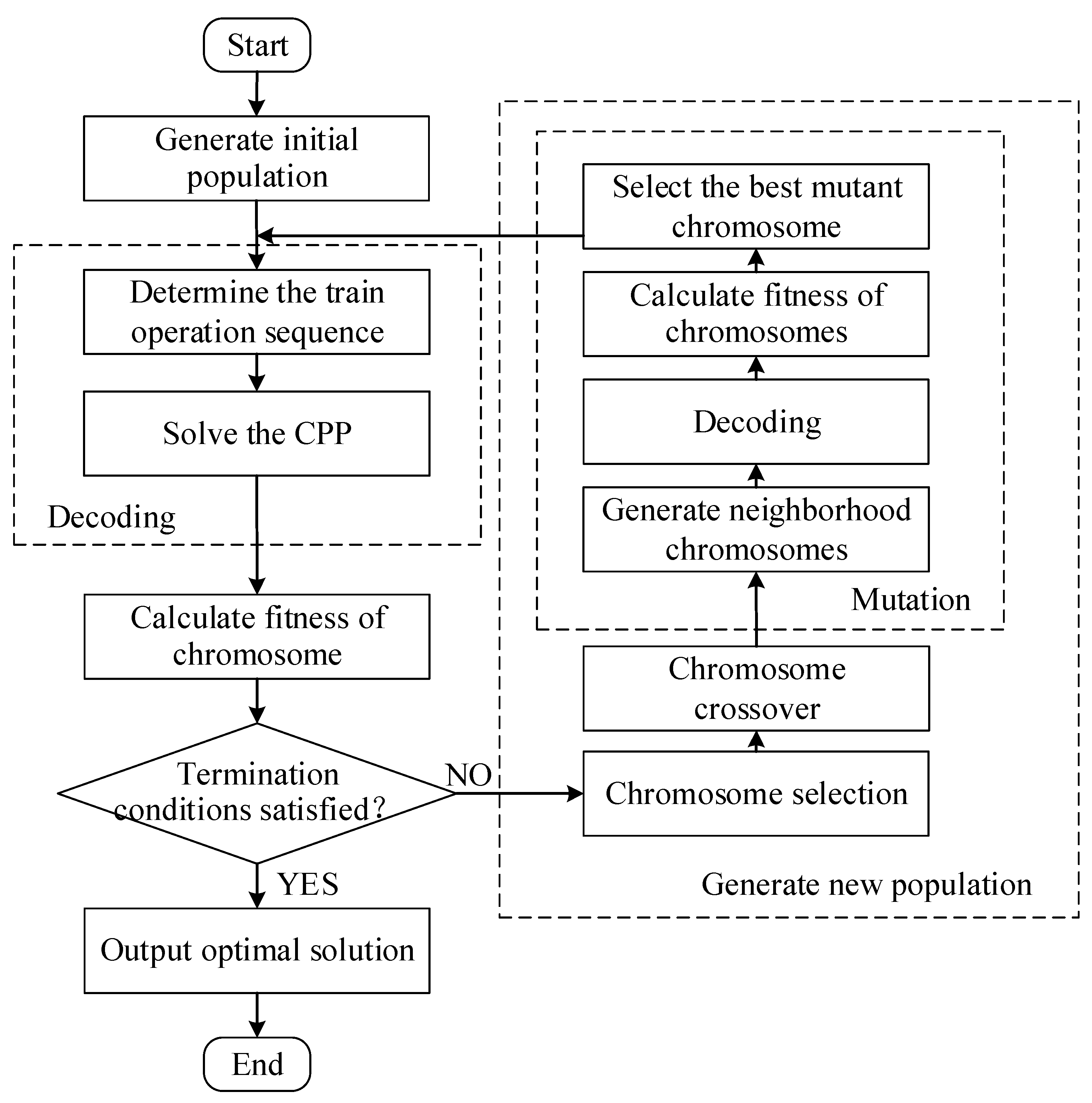
4.8. Algorithm

The framework of the algorithmic procedure is summarized below in Figure 7.

5. Case Study

This section provides several numerical experiments on the proposed heavy-haul railway train timetabling problem in order to prove the effectiveness of our models and algorithms.

5.1. A Small Case

In this section, we use a small case to illustrate the effectiveness of the proposed model and hybrid algorithm.

5.1.1. Operation Data

The corresponding schematic diagram of a small heavy-haul railway network is presented in Figure 8. As shown in the figure, this small heavy-haul railway consists of three loading stations (station a, station b, and station c), three unloading stations (station d, station e, and station f), and a CBS. The loading capacity of station a, station b, and station c is each 550 cars per day. The unloading demand of station d, station e, and station f is 360 cars/day, 720 cars/day, and 540 cars/day, respectively. Lastly, the unloading capacity of station d, station e, and station f can meet the unloading requirements.

In this small heavy-haul railway, the unit train types include 5 kt unit trains and 10 kt unit trains that contain 60 railcars and 120 railcars, respectively. The combined train types include 10 kt (2 × 5 kt) combined trains, 15 kt (3 × 5 kt) combined trans, and 20 kt (4 × 5 kt) combined trans. The corresponding combination rule and operation cost of these combined trans are 10 kt (2 × 5 kt) combined trans (two 5 kt unit trains, cost = 0.9), 15 kt (3 × 5 kt) combined trans (three 5 kt unit trains, cost = 1), and 20 kt (4 × 5 kt) combined trans (four 5 kt unit trains, cost = 1; or two 10 kt unit trains, cost = 1.8). The combined operation in the CBS should be during 0:00–8:00 and the combined train needs to depart from the CBS during 6:00–8:00.

5.1.2. Optimization Results

By solving the TSPP, we derive the type and number of unit trains that need to be loaded at each loading station, as well as the type and number of combined trains that need to be unloaded at each unloading station. The solution of the TSPP is shown in

Table 4. Solution of the TSPP in the small case.

Unloading Stations	Unit Train Type	Number of Trains	Loading Stations	Combined Train Type	Number of Trains
station a	5 kt	9	station d	10 kt (2 × 5 kt)	1
station b	5 kt	9	station d	20 kt (4 × 5 kt)	1
station c	5 kt	9	station e	20 kt (4 × 5 kt)	3
			station f	10 kt (2 × 5 kt)	1
			station f	15 kt (3 × 5 kt)	1
			station f	20 kt (4 × 5 kt)	1

. The TTP will be further solved based on this solution.

Then, we apply the proposed HGA to obtain the optimal combination scheme and train timetable to minimize the total dwell time of all heavy-haul trains. Specifically, some parameters of the HGA are set as follows:

• The crossover rate is set to 0.85;
• The mutation rate is set to 0.15 and the number of elements in the neighborhood set of mutation chromosomes is set as 20;
• The larger positive number M is set to 10,000; and
• When the optimal value exceeds 50 iterations without optimization, the iteration reaches the termination condition.

The corresponding results and the solution searching process of the small case are plotted in Figure 9. By generating and optimizing the combined operation plan of heavy-haul trains at the CBS, the total combined operation time in the system is 4664 car–hours.

In order to verify the effectiveness of the proposed model, we compare the results with the timetable obtained by the manual scheduling operation. To this end, we designed a simulation process to imitate the manual scheduling operation approaches of the heavy-haul railway scheduling system. The simulation steps are as follows:

Step 1: Assign a combination scheme of combined trains and unit trains based on experience.

Step 2: Randomly assign a series of the departure times of the combined trains in the CBS.

Step 3: Determine the arrival time of the unit trains at the CBS backwards according to the departure time of the combined trains and the required dwell time.

Step 4: Calculate trains’ arrival and departure times in each section according to the section running time.

Step 5: Check for conflicts and adjust the train timetable.

Next, the simulation method is applied to the small case to obtain a solution. The total dwell time obtained by the simulation is 7876 car–hours. Compared to the proposed model’s optimization results, the simulation method’s operation time increases by 3212 car–hours, resulting in a time waste of about 40.8%.

Figure 10 shows the combination scheme’s diagram using the HGA and the simulation. The horizontal axis shows the time and the vertical axis shows the position of the trains. These combination scheme diagrams can be divided into three parts. The upper oblique lines represent the unit trains running between the loading stations and the CBS. The lower oblique lines represent the combined trains running between the CBS and the unloading stations. The horizontal and vertical lines in the middle represent the combination relationship and the dwell time of each train. As shown in the figure, compared to the combination scheme obtained by the simulation, the solution obtained by the HGA is more compact and uses less time in the CBS.

To further compare the two methods, we calculate the waiting time of each unit train that waits for the combination operation in the two combination schemes. The waiting time is the period that lasts from when the unit train enters the CBS to when it starts the combination operation. The waiting time of each unit train in the CBS is shown in (20). We define the unit train whose waiting time in the CBS is less than 90 min as the efficient turnover train (ETT).

$$w_p={\displaystyle {\sum }_{p\in T^{com}}{d}_p\left(s_z,j\right){\theta }_{p,q}}-a_q\left(i,s_z\right),\forall q\in T^{uni}$$

(20)

Figure 11 plots the waiting time distribution of unit trains in the two solutions. The horizontal axis represents the index of the unit train and the vertical axis represents the waiting time of the corresponding unit train in the CBS. The green dotted line indicates that the waiting time is 90 min and the points below the green dotted line are the ETT. As shown in Figure 11, 18 unit trains in the combination scheme obtained by the TTP belong to the ETT, while only 7 ETT are in the combination scheme obtained by the simulation. Therefore, the combination scheme solved by the TTP can effectively reduce the waiting time of unit trains in the CBS, thus reducing the service load of stations and improving train turnover efficiency.

By comparing these two methods of scheduling the combination schemes, the efficiency of the TTP is verified.

5.1.3. Effectiveness of the Algorithm

In order to verify the effectiveness of the algorithm, we introduce an unimproved genetic algorithm (GA) and a tabu search (TS) to solve the optimization problem.

In experiments of GA, we still adopt the same representation scheme, population initialization operation, and chromosome-crossing operation as the method in this paper. The fitness function still adopts the reciprocal of the objective function. The difference is that the CPP is not called during the decoding process to find the optimized combination scheme. Meanwhile, the mutation operation uses single random mutation instead of neighborhood search.

As for the TS, it is another widely used stochastic search method designed to find the optimal solution. The tabu search algorithm imitates human memory and uses a tabu list to forbid certain moves to avoid cycling search [40]. The tabu search adopts neighborhood optimization. In order to transcend the local optimal solution, the algorithm can accept inferior solutions. In this algorithm, we use the same representation scheme in the HGA and we employ the neighborhood generation method of the mutation operator in the HGA. The objective function of the TTP is used as the evaluation function to evaluate the quality of neighbor solutions.

Then, we conducted five experiments with different parameters. Due to the randomness of the search process, we ran each experiment 10 times and calculated the average value of the best five solutions as the final result. The experimental parameters and results are shown in

Table 5. The parameters and results of the GA.

Index	Population Size	Generations	Crossover Rate	Mutation Rate	Total Operation Time (car–hours)
1	30	150	0.90	0.05	5735
2	50	200	0.80	0.1	5531
3	50	150	0.80	0.15	5623
4	80	250	0.75	0.15	5703
5	100	250	0.85	0.15	5537

,

Table 6. The parameters and results of the HGA.

Index	Population Size	Generations	Crossover Rate	Mutation Rate	Total Operation Time (car–hours)
1	30	150	0.90	0.05	4867
2	50	200	0.80	0.1	4855
3	50	150	0.80	0.15	4818
4	80	250	0.75	0.15	4770
5	100	250	0.85	0.15	4727

and

Table 7. The parameters and results of the TS.

Index	Number of Neighbors	Tabu Length	Iterations	Total Operation Time (car–hours)
1	20	15	200	5032
2	40	15	200	4993
3	40	10	200	5057

.

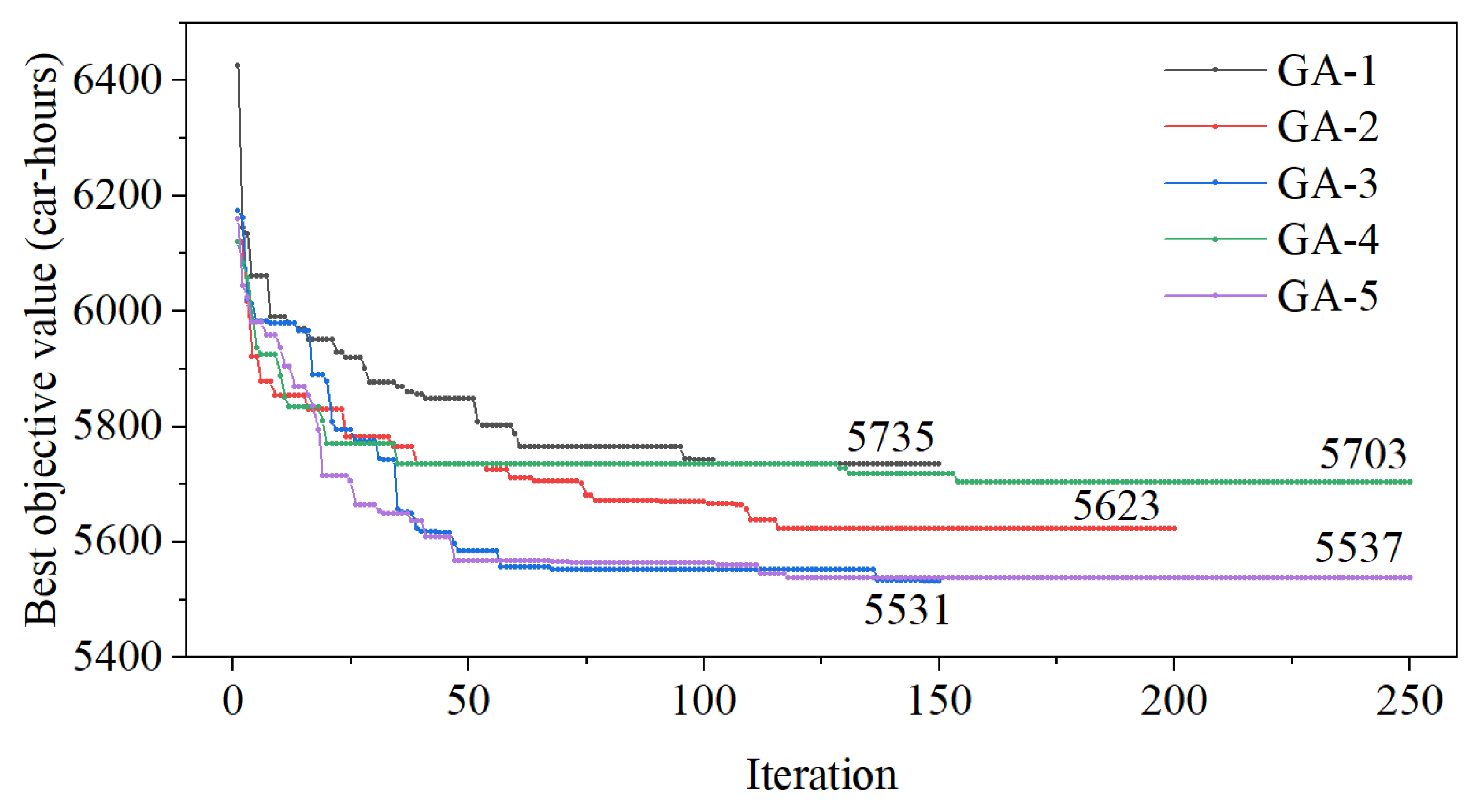
The search process of the two algorithms is shown in Figure 12, Figure 13 and Figure 14. All algorithms have made some progress in reducing the objective value. In the experimental group of the GA, experiment GA-3 obtained the best objective value, which was 5531 car–hours. In the experimental group of the HGA, the best objective function value was obtained in experiment HGA-4, which was 4727 car–hours. In the experimental group of the TS, the best objective function value was obtained in experiment TS-2, which was 4993 car–hours. In comparing Figure 12 with Figure 13, it is obvious that the HGA achieves better optimization values than the GA on the whole. As shown in Figure 14, compared with the TS, the HGA obtains a better initial solution and has a high convergence speed. The above experiments showed that, compared to the GA and TS, the HGA obtains a better initial solution because we solve the CPP model to improve the initial solution in the HGA. Additionally, the HGA achieves a high convergence speed. These experiments demonstrate the effectiveness of the designed HGA.

5.2. Large-Scale Experiments

5.2.1. Description of the Experimental Setting

To further show the effectiveness of the proposed approach, we select the Datong-Qinhuangdao Heavy-haul Railway (DQHR) as a large-scale study case. The DQHR, with a total length of 653 km, is China’s first double-line electrified heavy-haul railway and it is an important coal transportation corridor from Shanxi, Shaanxi, and western Inner Mongolia [41].

In these experiments, the DQHR contains 6 loading stations and 11 unloading stations. A simplified schematic is shown in Figure 15. Some important train operation parameters are listed in

Table 8. Parameters of the loading stations and unloading stations.

Parameters of Loading Stations		Parameters of Unloading Stations
Loading Station	Daily Loading Capacity (cars/day)	Unloading Station	Daily Unloading Capacity (cars/day)	Cargo Demand (cars/day)
Hanyuan	15,058	Gaogezhuang	382	300
Beitongpu	18,888	Duanjialing	870	500
Yungang	2365	Jixian	403	300
Kouquan	1134	Cuipingshan	960	600
Dabao	6845	Zunhuabei	1296	1000
Dahuai	7289	Qiananbei	480	300
		Caofeidian	4992	3000
		Donggang	1944	1500
		Luannan	4584	3500
		Houying	2544	1500
		Liucunnan	6720	4000

and

Table 9. The running cost and operating time of each type of combined train.

Index	Type of Combined Trains	Type and Number of Unit Trains	Cost of Train	Operating Time of Combination (min)
1	10 kt combined train	2 × 5 kt unit train	1.3	126
2	10 kt combined train	1 × 10 kt unit train	1	93
3	15 kt combined train	3 × 5 kt unit train	1.4	152
4	20 kt combined train	2 × 10 kt unit train	1.5	135
5	20 kt combined train	4 × 5 kt unit train	1.8	182
6	30 kt combined train	3 × 10 kt unit train	2	168

. Table 8 shows the capacity and demand of the loading and unloading stations in the DQHR. Table 8 shows the running cost and operating time of each type of combined train.

5.2.2. Computational Results of the Large-Scale Experiment

The solution of the TSPP in the large-scale experiment is shown in

Table 10. Solution of the TSPP in the large-scale experiment.

Unloading Stations	Unit Train Type	Number of Trains	Loading Stations	Combined Train Type	Number of Trains
Hanyuan	10 kt	24	Chawu	30 kt (3 × 10 kt)	1
Beitongpu	5 kt	114	Duanjialing	15 kt (3 × 5 kt)	3
Dahuai	5 kt	121	Jixian	30 kt (3 × 10 kt)	1
			Zunhua	15 kt (3 × 5 kt)	3
			Zunhua	20 kt (4 × 5 kt)	2
			Cuipingshan	15 kt (3 × 5 kt)	2
			Cuipingshan	20 kt (4 × 5 kt)	1
			Qianan	30 kt (3 × 10 kt)	1
			Caofeidian	15 kt (3 × 5 kt)	14
			Caofeidian	20 kt (4 × 5 kt)	2
			Donggang	15 kt (3 × 5 kt)	3
			Donggang	20 kt (4 × 5 kt)	4
			Luannan	15 kt (3 × 5 kt)	16
			Luannan	30 kt (3 × 10 kt)	2
			Houying	15 kt (3 × 5 kt)	7
			Houying	20 kt (4 × 5 kt)	1
			Liucunnan	15 kt (3 × 5 kt)	5
			Liucunnan	20 kt (4 × 5 kt)	9
			Liucunnan	30 kt (3 × 10 kt)	3

. Subsequent TTP will be further solved based on this solution.

In this large-scale experiment, the crossover rate was set to 0.85 and the mutation rate was set to 0.15. The number of elements in the neighborhood set of mutation chromosomes was set as 20. The maximum number of iterations was set to 200.

Figure 16 shows the iterative process of the HGA when used to solve the TTP in the large-scale experiment. As shown in Figure 16, the total combined operation time in the system was 98,848 car–hours. This example provides an illustration of the usefulness and application of our proposed approach.

6. Conclusions

Based on the actual demand of the heavy-haul railway, this paper proposes a scheduling approach to optimize the heavy-haul railway transportation plan, including the combination scheme and train timetable. This approach can satisfy the freight transportation demands, improve the utilization of the CBS operation, and reduce the cost of the whole transportation process, thus improving rail operators’ profits.

First, the train service plan problem (TSPP) model was proposed based on the loading stations’ capacity and the unloading stations’ demands. We solved the TSPP to determine the type and number of unit trains that need to be loaded at each loading station, as well as the type and number of combined trains that need to arrive and unload at unloading stations. On this basis, we put forward the train timetabling problem (TTP) model. The TTP model can solve the combination scheme in the CBS and the train timetable of the heavy-haul railway. Then, we applied a hybrid genetic algorithm (HGA) to solve the TTP model. In a small case study using the TTP model, we obtained a solution that reduces the total dwell time of unit trains by 40.8% compared to a manual scheduling simulation method. The comparison experiments with the unimproved genetic algorithm (GA) and tabu search (TS) demonstrate that the HGA can obtain better solutions and achieve a high convergence speed. By applying the approach into a large-scale case of DQHR, we demonstrated the practicability of the method in the real world.

In this paper, we assumed that the combined capacity of the CBS is large enough to deal with the unit trains. However, in practice, when the freight volume of the heavy-haul railway is too big, the CBS may not be able to combine many unit trains at once. In future studies, we will consider the combined capacity of the CBS as one of the constraints to determine a more feasible combination scheme. At the same time, the return and decomposed operation of the empty trains after the unloading operation is also a critical part of trains circulating in the heavy-haul railway system. Thus, the transportation organization of the empty trains will also be considered in future research.

References

- Fu, J.; Chen, J. A Green Transportation Planning Approach for Coal Heavy-Haul Railway System by Simultaneously Optimizing Energy Consumption and Capacity Utilization. Sustainability 2021, 13, 4173. [Google Scholar] [CrossRef]
- Zong, Y. Research on development countermeasures of railway coal transportation in China. Railw. Freight 2020, 38, 11–15. [Google Scholar]
- Fan, Z. Research on Car Flow Attractive Region of Heavy-Haul Channels and Direct Heavy-Haul Transportation; Beijing Jiaotong University: Beijing, China, 2008. [Google Scholar]
- Yang, Y.; Jia, C.; Hu, S. Relationship Determination with Train Weight, Speed, and Density of Heavy Haul Railway Line in China. J. Beijing Jiaotong Univ. 2006, 30, 1–4+9. [Google Scholar]
- Ma, H. Discussion on influencing factors of railway transportation capacity of Da-qin railway. J. Railw. Freight 2014, 8, 40–43. [Google Scholar]
- Sun, J.; Kong, L.; Pan, H. Develop Heavy-Loading Transportation and Increase Traffic Capacity of Baotou-Shenmu Railway. Transp. Logist. 2011, 20, 172–176. [Google Scholar]
- Zhou, F. Research on Key Technologies of Baoshen Railway Heavy Haul Transportation Organization; Lanzhou Jiaotong University: Lanzhou, China, 2019. [Google Scholar]
- Xue, F.; Zhao, L.; Fan, Q. Study on coupling and adjustment of marshalling yard stage plan and dynamic traffic flow. J. China Railw. Soc. 2020, 42, 18–26. [Google Scholar]
- Wang, C. Application of goal programming in railway heavy haul transportation. J. Southwest Jiaotong Univ. 2009, 44, 392–395. [Google Scholar]
- Zhao, P.; Zhang, J.; Tang, B. Study on the Optimization Model of Car Flow Organization in the Loading Area of Heavy Haul Railway Based on the Combined Trains. China Railw. Sci. 2010, 31, 116–121. [Google Scholar]
- Tang, B. Study on the Organization of Wagon Flow in Heavy Haul Loading Area; Beijing Jiaotong University: Beijing, China, 2009. [Google Scholar]
- Wang, W. Research on the Organization of Direct Wagon Flow in Heavy-Haul Loading Area; Southwest Jiaotong University: Chengdu, China, 2012. [Google Scholar]
- Jing, L.; LI, G. Research on traffic organization optimization of heavy haul transportation based on improved fruit fly algorithm. Railw. Transp. Econ. 2018, 40, 30–35. [Google Scholar]
- Xiao, J.; Lin, B.; Wang, J. Solving the train formation plan network problem of the single-block train and two-block train using a hybrid algorithm of genetic algorithm and tabu search. Transp. Res. Part C Emerg. Technol. 2018, 86, 124–146. [Google Scholar] [CrossRef]
- China Railway Publishing House. Specification for the design of heavy-haul railways: TB 10625—2017[S]. In China, National Railway Administration of the People’s Republic of China; China Railway Publishing House: Beijing, China, 2017. [Google Scholar]
- Zhiye, W.; Bing, Z. Study of Schematic Design of Technical Operation Stations for Heavy Haul Railway. China Railw. 2019, 06, 71–76. [Google Scholar]
- Wei, Y.; Zhang, H.; Yang, H. Impact of Turnout Type Selection on Station Carrying Capacity of Heavy Haul Railway. China Railw. Sci. 2013, 34, 95–98. [Google Scholar]
- Ye, J.; Wang, H. Practice and development of 20,000 T combined train in Hudong Station. China Railw. 2009, 6, 22–25. [Google Scholar]
- Liang, Q.; Han, D.; Zhang, J. The influence of 20,000 T heavy haul train on the arrival and departure of Hudong Marshalling Station of Daqin Line. China Railw. Sci. 2005, 26, 1–6. [Google Scholar]
- Han, X.; Guo, H.; Peng, Q. Methods for optimization of combination schemes of combination stations in heavy-haul transportation. J. China Railw. Soc. 2012, 34, 1–7. [Google Scholar]
- Ma, M.; Ding, D.; Ren, Z. Optimal Utilization of Arrival and Departure Track in Heavy Haul Railways. Railw. Investig. 2019, 45, 110–115. [Google Scholar]
- Yaghini, M.; Momeni, M.; Sarmadi, M. A hybrid solution method for fuzzy train formation planning. Appl. Soft Comput. 2015, 31, 257–265. [Google Scholar] [CrossRef]
- Martinelli, D.R.; Teng, H. Optimization of railway operations using neural networks. Transp. Res. Part C Emerg. Technol. 1996, 4, 33–49. [Google Scholar] [CrossRef]
- Kozachenko, D.; Bobrovskiy, V.; Gera, B.; Skovron, I.; Gorbova, A. An optimization method of the multi-group train formation at flat yards. Int. J. Rail Transp. 2020, 9, 61–78. [Google Scholar] [CrossRef]
- Lin, B.-L.; Wang, Z.-M.; Ji, L.-J.; Tian, Y.-M.; Zhou, G.-Q. Optimizing the freight train connection service network of a large-scale rail system. Transp. Res. Part B Methodol. 2012, 46, 649–667. [Google Scholar] [CrossRef]
- Lin, B.; Zhao, Y. The Systematic Optimization of Train Formation in Loading Stations. Symmetry 2019, 11, 1238. [Google Scholar] [CrossRef] [Green Version]
- Yaghini, M.; Momeni, M.; Sarmadi, M. Solving train formation problem using simulated annealing algorithm in a simplex framework. J. Adv. Transp. 2014, 48, 402–416. [Google Scholar] [CrossRef]
- Murali, P.; Ordóñez, F.; Dessouky, M.M. Modeling strategies for effectively routing freight trains through complex networks. Transp. Res. Part C Emerg. Technol. 2016, 70, 197–213. [Google Scholar] [CrossRef]
- Lazarev, A.A.; Musatova, E.G. The problem of trains formation and scheduling: Integer statements. Autom. Remote Control 2013, 74, 2064–2068. [Google Scholar] [CrossRef]
- Ma, X. Research on the Organization Mode of Railway Heavy Load Transportation and Related Problems; Southwest Jiaotong University: Chengdu, China, 2006. [Google Scholar]
- Tong, L.; Zhou, L.; Liu, J.; Zhou, X. Customized bus service design for jointly optimizing passenger-to-vehicle assignment and vehicle routing. Transport. Res. C-Emerg. Technol. 2017, 85, 451–475. [Google Scholar] [CrossRef]
- Yue, Y.; Wang, S.; Zhou, L.; Tong, L.; Saat, M.R. Optimizing train stopping patterns and schedules for high-speed passenger rail corridors. Transport. Res. C-Emerg. Technol. 2016, 63, 126–146. [Google Scholar] [CrossRef]
- Zhang, Y.; D’Ariano, A.; He, B.; Peng, Q. Microscopic optimization model and algorithm for integrating train timetabling and track maintenance task scheduling. Transp. Res. Part B Methodol. 2019, 127, 237–278. [Google Scholar] [CrossRef]
- Oroojlooy Jadid, A.; Eshghi, K. Train Timetabling on double track and multiple station capacity railway with useful upper and lower bounds. Sci. Iran 2017, 24, 3324–3344. [Google Scholar] [CrossRef] [Green Version]
- Holland, J.H. Adaption in Natural and Artificial Systems; The MIT Press: Cambridge, CA, USA, 1975; Volume 6, pp. 126–137. [Google Scholar]
- Man, K.F.; Tang, K.S.; Kwong, S. Genetic algorithms: Concepts and applications. IEEE Trans. Ind. Electron. 1996, 43, 519–534. [Google Scholar] [CrossRef]
- Coley, D.A. Genetic algorithms. Contemp. Phys. 1996, 37, 145–154. [Google Scholar] [CrossRef]
- Zhou, Y.; Zhou, L.; Wang, Y.; Yang, Z.; Wu, J. Application of Multiple-Population Genetic Algorithm in Optimizing the Train-Set Circulation Plan Problem. Complexity 2017, 2017, 3717654. [Google Scholar] [CrossRef] [Green Version]
- Glover, F.; Kelly, J.P.; Laguna, M. Genetic algorithms and tabu search: Hybrids for optimization. Comput. Oper. Res. 1995, 22, 111–134. [Google Scholar] [CrossRef]
- Glover, F. Future paths for integer programming and links to artificial intelligence. Comput. Oper. Res. 1986, 13, 533–549. [Google Scholar] [CrossRef]
- Ma, J. Research on Countermeasures for Improving Freight Capacity of Daqin Railway line. Railw. Freight 2021, 39, 1–6. [Google Scholar]
Figure 1.
The relations between stages in the decision-making process of the heavy-haul railway transportation plan.
Figure 2.
Simplified schematic diagram of a heavy-haul railway.
Figure 3.
The operating process of trains in a heavy-haul railway network.
Figure 4.
The operating process of heavy-haul trains in a space–time network.
Figure 5.
The framework of the heavy-haul train timetabling methodology.
Figure 6.
Gene fragments of the combined operation.
Figure 7.
Flow chart of the solution approach.
Figure 8.
Simplified heavy-haul railway network of the small case.
Figure 9.
The solution searching process of the small case using the HGA.
Figure 10.
The comparison of the results of the two methods: (a) the diagram of the combination scheme using the HGA and (b) the diagram of the combined combination scheme using the simulation.
Figure 11.
The distribution of the waiting time for unit trains in the two solutions.
Figure 12.
The solution searching process of the GA.
Figure 13.
The solution searching process of the HGA.
Figure 14.
The solution searching process of the TS.
Figure 15.
Simplified Datong-Qinhuangdao Heavy-haul Railway.
Figure 16.
The solution searching process of the large-scale experiment using the HGA.