
The Due Date Assignment Scheduling Problem with Delivery Times and Truncated Sum-of-Processing-Times-Based Learning Effect

College of Science, Northeastern University, Shenyang 110819, China
*
Author to whom correspondence should be addressed.
Mathematics 2021, 9(23), 3085; https://0-doi-org.brum.beds.ac.uk/10.3390/math9233085
Submission received: 28 October 2021
/
Revised: 26 November 2021
/
Accepted: 26 November 2021
/
Published: 30 November 2021
(This article belongs to the Special Issue Applied Computing and Artificial Intelligence)
Abstract
:This paper considers a single-machine scheduling problem with past-sequence-dependent delivery times and the truncated sum-of-processing-times-based learning effect. The goal is to minimize the total costs that comprise the number of early jobs, the number of tardy jobs and due date. The due date is a decision variable. There will be corresponding penalties for jobs that are not completed on time. Under the common due date, slack due date and different due date, we prove that these problems are polynomial time solvable. Three polynomial time algorithms are proposed to obtain the optimal sequence.
1. Introduction
Scheduling problems are widely used in manufacturing, logistics, and other practical applications. For a real-word example of our scheduling problems, consider a processing enterprise that has no inventory capacity. As the processing time increases, the processing technology improves. The processing time of the product becomes shorter. The pick-up time of each product is determined by the customer. If the product is produced before the pick-up time or after the pick-up time, an additional delivery fee will be incurred. The delivery price of each early (tardy) job is a fixed charge.
The following three forms of pick-up time are often considered:
- (1)
- All products have a uniform delivery time;
- (2)
- The pick-up time of each product is related to its own processing time and a constant;
- (3)
- Each product has its own independent pick-up time.
The scheduling problem is a very classic discrete combinatorial optimization problem. The methods to solve the scheduling problem mainly include two types: the exact algorithm and approximate algorithm. Exact algorithms mainly include mathematical programming methods, dynamic programming, and branch and bound algorithms. Approximate algorithms mainly include heuristic algorithms and intelligent algorithms. For large-scale non-polynomial time-solvable scheduling problems, intelligent algorithms and machine learning algorithms can be used to solve them. In this paper, a single-machine scheduling problem is considered that contains due dates, the delivery time and learning effect. The actual processing time of a job is a learning function of the previous processing time. The objective function is to minimize the number of early jobs, the number of tardy jobs and due date. Under the common due date, slack due date and different due date, three polynomial time algorithms are proposed to obtain the optimal sequence.
2. Literature Review
In traditional scheduling problems, it is considered that the processing time of jobs is constant. However, in reality, the processing time is often reduced with the increase in workers’ skills and abilities. That means the processing time is no longer a constant. In 2011, Cheng et al. developed the branch-and-bound algorithm and simulated an annealing algorithm in order to study the single-machine scheduling problem with a learning effect and truncation processing time [1]. In 2013, Li et al. analyzed the polynomial time algorithm of the single-machine scheduling problem with a truncation processing time [2]. In 2013, Cheng et al. used a genetic algorithm and branch-and-bound algorithm to solve the two-machine flow-shop scheduling problem with a truncated learning function [3]. In 2016, Wu and Wang studied a single-machine scheduling problem with a learning effect and delivery times [4]. In 2017, Wang et al. solved the single-machine scheduling problem with resource allocation and deterioration effects by using the polynomial time algorithm [5]. In 2018, Wu et al. studied a two-stage scheduling problem with a position-based learning effect [6]. In 2018, Yin studied a single-scheduling problem with resource allocation and a learning effect [7]. In 2020, Zhang studied the scheduling problem with the sum-of-processing-times-based learning effect [8]. In 2020, Qian et al. designed a heuristic algorithm to study the single-scheduling problem with release times and a learning factor [9]. In 2020, Zou et al. studied a multi-machine scheduling problem with the sum-of-processing-times-based learning effect [10]. In 2021, Wu et al. studied a flow-shop scheduling problem with a truncated learning function [11].
In the field of scheduling, the delivery time has attracted extensive attention. The extra time required for a completed job to be delivered to the customer is called the p ast-sequence-dependent (psd) delivery time. In 2011, Yang et al. studied a single-machine scheduling problem with delivery times and a learning effect [12]. In 2012, Yang et al. studied a single-machine scheduling problem with delivery times and position-dependent processing times [13]. In 2013, Liu studied a scheduling problem with delivery times and deteriorating jobs [14]. In 2014, Zhao et al. studied a single-machine scheduling problem with delivery times and general position-dependent processing times [15]. In 2021, Qian et al. studied a single-machine scheduling problem with delivery times and deteriorating jobs [16].
In actual production scheduling, the jobs often have due dates. If a job is completed ahead of the due date, it will have an earliness cost; if a job is completed behind the due date, it will have a tardiness cost. In 2013, Yin et al. studied a single-machine scheduling problem with a due date, delivery times and learning effect [17]. In 2014, Lu et al. studied a single-machine scheduling problem with a due date, learning effect and resource allocation [18]. In 2015, Li et al. studied a single-machine scheduling problem with a slack due window, learning effect and resource allocation [19]. In 2016, Sun et al. studied a single-machine scheduling problem with a due date and convex resource allocation [20]. In 2019, Geng et al. studied a flow-shop scheduling problem with a common due date, resource allocation and learning effect [21]. In 2020, Liu et al. studied a single-machine scheduling problem with a due date, learning effect and resource allocation [22]. In 2021, Tian studied a single-machine scheduling problem with resource allocation and generalized earliness–tardiness penalties [23]. In 2021, Wang studied a single-machine scheduling problem with proportional setup times and earliness–tardiness penalties [24]. In 1996, Lann et al. studied a single-machine scheduling problem whose goal was to minimize the number of early and tardy jobs [25]. In 2017, Yuan studied a single-machine scheduling problem to minimize the number of tardy jobs [26]. In 2021, Hermelin studied a single-machine scheduling problem to minimize the weighted number of tardy jobs [27].
3. Notation and Problem Statement
Some notations used in this paper are introduced in Table 1.
Suppose there were n independent jobs continuously processed on a single machine. The machine can handle one job at a time. The actual processing time of at the kth position was:
The delivery time of was:
where . The completion time of :
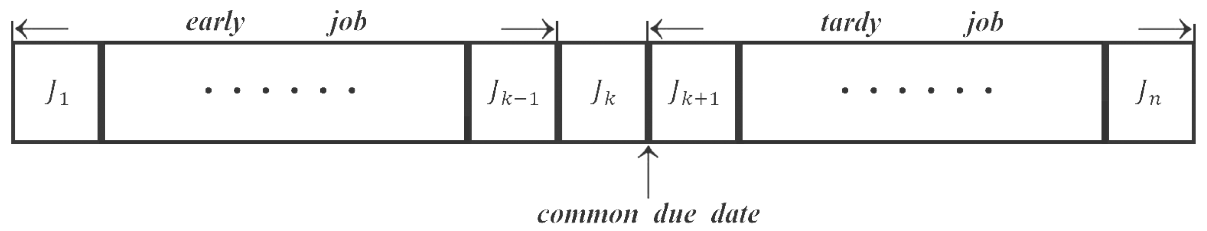
The common due date, slack due date and different due date were considered in this paper. For the CON model, the due date of each job was the same. For the SLK model, the due date was the sum of the processing time and certain parameter q. For the DIF model, each job had its own due date. The due date was a decision variable. If was an early job, , . If was a tardy job, , . By the three-field notation [28], the models could be defined as:
where represents the past-sequence-dependent delivery times. The following Figure 1 shows the just-in-time common due date scheduling model.
4. Research Method
Lemma 1.
Lemma 2.
4.1. The Problem
Lemma 3.
For any job sequence, the due date d of the optimal scheduling was the completion time of some job.
Proof.
Suppose that the due date d of the optimal scheduling was not equal to the completion time of some job, i.e., , , . The objective function was:
When d was equal to , the objective function was:
Therefore, d was the completion time of some job. □
Lemma 4.
When , the due date d was equal to 0.
Proof.
When the due date d was equal to , the objective function was:
- (1)
- When d was equal to , the objective function was:
- (2)
- When d was equal to , the objective function was:
when ,
. Therefore, the due date d was equal to the start time of the first job. □
For the convenience of proof, we defined two sets: , , .
Lemma 5.
In the optimal scheduling, the jobs of set were arranged in an ascending order of normal processing time.
Proof.
There were two adjacent jobs and in the , and was in front of which was at the th position, . Suppose that the starting time of was 0, , . The objective function of was:
when and were swapped, the sequence of jobs was . The objective function of was:
From and Lemma 2, , i.e., the jobs of set were arranged in an ascending order of normal processing time. □
Lemma 6.
In the optimal scheduling, the jobs of set were arranged in any order of normal processing time.
Proof.
There were two adjacent jobs and in the , and was in front of which was at the th position, , . The objective function of was:
when and were swapped, the sequence of jobs was . The objective function of was:
Therefore, the jobs of set were arranged in any order of normal processing time. □
Lemma 7.
In the optimal scheduling, the processing time of any job in the was less than the processing time of any job in the .
Proof.
There were two adjacent jobs and , was at the hth position in the , and was at the th position in the , . The objective function of was:
when and were swapped, the sequence of jobs was . The objective function of was:
If , , i.e., the processing time of any job in the was less than the processing time of any job in the . □
The Algorithm 1 was summarized as follows:
| Algorithm 1 |
| Require:, , , , a, r, , n Ensure: The optimal sequence, d
|
Theorem 1.
For the problem , the complexity of the algorithm was .
Proof.
The first step required time. The second step required time. The third step was completed in a constant time. Therefore, the complexity of the algorithm was . □
4.2. The Problem
Lemma 8.
For the optimal scheduling, q was equal to times the sum of actual processing time for some jobs.
Proof.
Suppose that q was not equal to times the sum of the actual processing time for some jobs, i.e., , , . The objective function was:
when , the objective function was:
Therefore, q was equal to times the sum of the actual processing time for some jobs. □
Lemma 9.
When , q was equal to 0.
Proof.
when , . Therefore, q was equal to 0. □
When q was equal to for the optimal scheduling, the objective function was:
- (1)
- When , the objective function was
- (2)
- When , the objective function was
For the convenience of proof, we defined two sets: , , .
Lemma 10.
In the optimal scheduling, the jobs of set were arranged in an ascending order of normal processing time.
Proof.
There were two adjacent jobs and in the , and was in front of which was at the th position, . Suppose that the starting time of was 0, , . The objective function of was:
when and were swapped, the sequence of jobs was . The objective function of was:
From and Lemma 1, , i.e., the jobs of set were arranged in an ascending order of normal processing time. □
Lemma 11.
In the optimal scheduling, the jobs of set were arranged in an ascending order of normal processing time.
Proof.
There were two adjacent jobs and in the , and was in front of which was at the th position, , . The objective function of was:
when and were swapped, the sequence of jobs was . The objective function of was:
Therefore, the jobs of set were arranged in any order of normal processing time. □
Lemma 12.
In the optimal scheduling, the processing time of any job in the was less than the processing time of any job in the .
Proof.
There were two adjacent jobs and , and was at the th position in the , and was at the hth position in the , . The objective function of was:
when and were swapped, the sequence of jobs was . The objective function of was:
If , , i.e., the processing time of any job in the was less than the processing time of any job in the . □
The Algorithm 2 was summarized as follows:
| Algorithm 2 |
| Require:, , , , a, r, , n Ensure: The optimal sequence, q
|
Theorem 2.
For the problem , the complexity of the algorithm was .
Proof.
The first step required time. The second step required time. The third step was completed in a constant time. Therefore, the complexity of the algorithm was . □
4.3. The Problem
Lemma 13.
In the optimal scheduling, if , the due date of was equal to 0; otherwise, was equal to the completion time of .
Proof.
The objective function was:
- (1)
- When ,
- (2)
- When ,
- (3)
- When ,
when , was equal to 0; otherwise, was equal to . □
Lemma 14.
In the optimal scheduling, the jobs were sequenced in an increasing order of normal processing time.
Proof.
We considered the job sequence . There were two adjacent jobs and . was at the kth position in the and was at the th position in the , . was the objective function of . When and were swapped, the sequence of jobs was . was the objective function of .
From and Lemma 1, , , . Therefore, the jobs were sequenced in an increasing order of normal processing time in the optimal scheduling. □
The Algorithm 3 was summarized as follows:
| Algorithm 3 |
| Require:, , , , a, r, , n Ensure: The optimal sequence,
|
Theorem 3.
For the problem , the complexity of the algorithm was .
Proof.
The first step required time. The second step required time. Therefore, the complexity of the algorithm was . □
5. Discussion of Results
5.1. Numerical Discussion
In this section, we used an example to show the calculation process for three different due dates.
Example 1.
There were five jobs processed sequentially on the same machine. The processing time of each job is shown in the Table 2, Table 3, Table 4, Table 5, Table 6, Table 7, Table 8, Table 9, Table 10, Table 11, Table 12, Table 13, Table 14, Table 15, Table 16, Table 17, Table 18, Table 19 and Table 20 below:
, , , , , .
Solution 1:
First step: . The processing sequence of jobs: .
Second step:
- (1)
- When , , ;
- (2)
- When , , ;
- (3)
- When , , ;
- (4)
- When , , ;
- (5)
- When , , ;
- (6)
- When , , .
Third step: The optimal due date was 1.
Solution 2:
First step: . The processing sequence of jobs: .
Second step:
- (1)
- When , , ;
- (2)
- When , , ;
- (3)
- When , , ;
- (4)
- When , , ;
- (5)
- When , , ,
Third step: The optimal q was 0.
Solution 3:
First step: . The processing sequence of jobs: .
Second step: .
5.2. Extension
In the learning effect scheduling model, the learning index a was less than 0. If , it became the forgetting effect scheduling model.
where . The same method could prove the following conclusions. When , the optimal sequence was obtained by the longest processing time order. When , the optimal sequence was obtained by the shortest processing time order. Take Example 1 above as an example to show the algorithmic process of the forgetting effect scheduling model (CON).
Solution 4: where .
First step: . The processing sequence of jobs: .
Second step:
- (1)
- When , , ;
- (2)
- When , , ;
- (3)
- When , , ;
- (4)
- When , , ;
- (5)
- When , , ;
- (6)
- When , , .
Third step: The optimal due date was 0.
6. Conclusions
Under the common due date, slack due date and different due date, a single-machine scheduling problem with delivery times and the truncated sum-of-processing-times-based learning effect was studied in this paper. The goal was to minimize the total costs that comprised the number of early jobs, the number of tardy jobs and the due date. Under different due dates, three polynomial time algorithms were proposed to obtain the optimal sequence and due dates, whose complexity was . The optimal sequence was arranged in an ascending order of processing time. We gave three examples to show the calculation process of the algorithms. In the future, the multi-machine environment could be considered to expand the research, i.e., a flow-shop scheduling problem with a delivery time, truncated sum-of-processing-times-based learning effect and due dates could be considered whether there were polynomial time algorithms. The truncated sum-of-processing-times-based forgetting effect was also studied in the single-machine scheduling environment.
Author Contributions
The work presented here was performed in collaboration among all authors. J.Q. designed, analyzed and wrote the paper. Y.Z. analyzed and reviewed the paper. All authors have read and agreed to the published version of the manuscript.
Funding
This study was supported by the Natural Science Foundation of Liaoning Province Project (grant no. 2021-MS-102) and the Fundamental Research Funds for the Central Universities (grant no. N2105021 and N2105020).
Data Availability Statement
Not applicable.
Acknowledgments
We thank the anonymous reviewers for their comments and insights that significantly improved our paper.
Conflicts of Interest
The authors declare no conflict of interest.
References
- Cheng, T.C.E.; Cheng, S.R.; Wu, W.H.; Hsu, P.H.; Wu, C.C. A two-agent single-machine scheduling problem with truncated sum-of-processing-times-based learning considerations. Comput. Ind. Eng. 2011, 60, 534–541. [Google Scholar] [CrossRef]
- Li, L.; Yang, S.W.; Wu, Y.B.; Huo, Y.Z.; Ji, P. Single machine scheduling jobs with a truncated sum-of-processing-times-based learning effect. Int. J. Adv. Manuf. Technol. 2013, 67, 261–267. [Google Scholar] [CrossRef]
- Cheng, T.C.E.; Wu, C.C.; Chen, J.C.; Wu, W.H.; Cheng, S.R. Two-machine flowshop scheduling with a truncated learning function to minimize the makespan. Int. J. Prod. Econ. 2013, 141, 79–86. [Google Scholar] [CrossRef]
- Wu, Y.B.; Wang, J.J. Single-machine scheduling with truncated sum-of-processing-times-based learning effect including proportional delivery times. Neural Comput. Appl. 2016, 27, 937–943. [Google Scholar] [CrossRef]
- Wang, J.B.; Liu, M.; Yin, N. Scheduling jobs with controllable processing time, truncated job-dependent learning and deterioration effects. J. Ind. Manag. Optim. 2017, 13, 1025. [Google Scholar] [CrossRef] [Green Version]
- Wu, C.C.; Wang, D.J.; Cheng, S.R.; Chung, I.H.; Lin, W.C. A two-stage three-machine assembly scheduling problem with a position-based learning effect. Int. J. Prod. Res. 2018, 56, 3064–3079. [Google Scholar] [CrossRef]
- Yin, N. Single machine due window assignment resource allocation scheduling with job-dependent learning effect. J. Appl. Math. Comput. 2018, 56, 715–725. [Google Scholar] [CrossRef]
- Zhang, X. Single machine and flowshop scheduling problems with sum-of-processing time based learning phenomenon. J. Ind. Manag. Optim. 2020, 16, 231. [Google Scholar] [CrossRef] [Green Version]
- Qian, J.; Lin, H.; Kong, Y.; Wang, Y. Tri-criteria single machine scheduling model with release times and learning factor. Appl. Math. Comput. 2020, 387, 124543. [Google Scholar] [CrossRef]
- Zou, Y.; Wang, D.; Lin, W.C.; Chen, J.Y.; Yu, P.W.; Wu, W.H.; Chao, Y.P.; Wu, C.C. Two-stage three-machine assembly scheduling problem with sum-of-processing-times-based learning effect. Soft Comput. 2020, 24, 5445–5462. [Google Scholar] [CrossRef]
- Wu, C.C.; Zhang, X.; Azzouz, A.; Shen, W.L.; Cheng, S.R.; Hsu, P.H.; Lin, W.C. Metaheuristics for two-stage flow-shop assembly problem with a truncation learning function. Eng. Optim. 2021, 53, 843–866. [Google Scholar] [CrossRef]
- Yang, S.J.; Hsu, C.J.; Chang, T.R.; Yang, D.L. Single-machine scheduling with past-sequence-dependent delivery times and learning effect. J. Chin. Inst. Ind. Eng. 2011, 28, 247–255. [Google Scholar] [CrossRef]
- Yang, S.J.; Yang, D.L. Single-machine scheduling problems with past-sequence-dependent delivery times and position-dependent processing times. J. Oper. Res. Soc. 2012, 63, 1508–1515. [Google Scholar] [CrossRef]
- Liu, M.; Wang, S.; Chu, C. Scheduling deteriorating jobs with past-sequence-dependent delivery times. Int. J. Prod. Econ. 2013, 144, 418–421. [Google Scholar] [CrossRef]
- Zhao, C.; Tang, H. Single machine scheduling problems with general position-dependent processing times and past-sequence-dependent delivery times. J. Appl. Math. Comput. 2014, 45, 259–274. [Google Scholar] [CrossRef]
- Qian, J.; Han, H. The due date assignment scheduling problem with the deteriorating jobs and delivery time. J. Appl. Math. Comput. 2021, 1–14, in press. [Google Scholar] [CrossRef]
- Yin, Y.; Liu, M.; Cheng, T.C.E.; Wu, C.C.; Cheng, S.R. Four single-machine scheduling problems involving due date determination decisions. Inf. Sci. 2013, 251, 164–181. [Google Scholar] [CrossRef]
- Lu, Y.Y.; Li, G.; Wang, Y.B.; Ji, P. Optimal due-date assignment problem with learning effect and resource-dependent processing times. Optim. Lett. 2014, 8, 113–127. [Google Scholar] [CrossRef]
- Li, G.; Luo, M.L.; Zhang, W.J.; Wang, X.Y. Single-machine due-window assignment scheduling based on common flow allowance, learning effect and resource allocation. Int. J. Prod. Res. 2015, 53, 1228–1241. [Google Scholar] [CrossRef]
- Sun, L.H.; Cui, K.; Chen, J.H.; Wang, J. Due date assignment and convex resource allocation scheduling with variable job processing times. Int. J. Prod. Res. 2016, 54, 3551–3560. [Google Scholar] [CrossRef]
- Geng, X.N.; Wang, J.B.; Bai, D. Common due date assignment scheduling for a no-wait flowshop with convex resource allocation and learning effect. Eng. Optim. 2019, 51, 1301–1323. [Google Scholar] [CrossRef]
- Liu, W.; Jiang, C. Due-date assignment scheduling involving job-dependent learning effects and convex resource allocation. Eng. Optim. 2020, 52, 74–89. [Google Scholar] [CrossRef]
- Tian, Y. Single–Machine Due-Window Assignment Scheduling with Resource Allocation and Generalized Earliness/Tardiness Penalties. Asia-Pac. J. Oper. Res. 2021, in press. [Google Scholar] [CrossRef]
- Wang, W. Single-machine due-date assignment scheduling with generalized earliness-tardiness penalties including proportional setup times. J. Appl. Math. Comput. 2021, in press. [Google Scholar] [CrossRef]
- Lann, A.; Mosheiov, G. Single machine scheduling to minimize the number of early and tardy jobs. Comput. Oper. Res. 1996, 23, 769–781. [Google Scholar] [CrossRef]
- Yuan, J. Unary NP-hardness of minimizing the number of tardy jobs with deadlines. J. Sched. 2017, 20, 211–218. [Google Scholar] [CrossRef]
- Hermelin, D.; Karhi, S.; Pinedo, M.; Shabtay, D. New algorithms for minimizing the weighted number of tardy jobs on a single machine. Ann. Oper. Res. 2021, 298, 271–287. [Google Scholar] [CrossRef] [Green Version]
- Graham, R.L.; Lawler, E.L.; Lenstra, J.K.; Kan, A.H.G.R. Optimization and approximation in deterministic sequencing and scheduling: A survey. Ann. Discret. Math. 1979, 5, 287–326. [Google Scholar]
Figure 1.
The just-in-time CON scheduling model.


Table 1.
Symbol definition.
| Symbol | Meaning |
|---|---|
| n | the number of jobs |
| the normal processing time of | |
| the normal processing time for the jth position | |
| the actual processing time of | |
| the waiting time of | |
| the completion time of | |
| the makespan | |
| the delivery time of | |
| d | the due date |
| a | the learning index, |
| r | the delivery rate, |
| the truncation parameter, | |
| the weights | |
| the job arranged at the jth position | |
| CON | the common due date |
| SLK | the slack due date |
| DIF | the different due date |
Table 2.
Normal processing time.
| Job | |||||
|---|---|---|---|---|---|
| 4 | 3 | 5 | 2 | 1 |
Table 3.
Actual processing time.
| Value | 1 | 1 | 1.5 | 2 | 2.5 |
Table 4.
Waiting time.
| Value | 0 | 1 | 2 | 3.5 | 5.5 |
Table 5.
Delivery time.
| Value | 0 | 0.1 | 0.2 | 0.35 | 0.55 |
Table 6.
Completion time.
| Value | 1 | 2.1 | 3.7 | 5.85 | 8.55 |
Table 7.
Actual processing time.
| Value | 1 | 1 | 1.5 | 2 | 2.5 |
Table 8.
Waiting time.
| Value | 0 | 1 | 2 | 3.5 | 5.5 |
Table 9.
Delivery time.
| Value | 0 | 0.1 | 0.2 | 0.35 | 0.55 |
Table 10.
Completion time.
| Value | 1 | 2.1 | 3.7 | 5.85 | 8.55 |
Table 11.
Due date.
| Value | 1 | 1 | 1.5 | 2 | 2.5 |
Table 12.
Due date.
| Value | 2.1 | 2.1 | 2.6 | 3.1 | 3.6 |
Table 13.
Due date.
| Value | 3.2 | 3.2 | 3.7 | 4.2 | 4.7 |
Table 14.
Due date.
| Value | 4.85 | 4.85 | 5.35 | 5.85 | 6.35 |
Table 15.
Due date.
| Value | 7.05 | 7.05 | 7.55 | 8.05 | 8.55 |
Table 16.
Due date.
| Value | 1 | 2.1 | 3.7 | 5.85 | 8.55 |
Table 17.
Actual processing time.
| Value | 5 | 9.8 | 9.49 | 7.21 | 3.87 |
Table 18.
Waiting time.
| Value | 0 | 5 | 14.8 | 24.29 | 31.5 |
Table 19.
Delivery time.
| Value | 0 | 0.5 | 1.48 | 2.429 | 3.15 |
Table 20.
Completion time.
| Value | 5 | 15.3 | 25.76 | 33.929 | 38.52 |
Publisher’s Note: MDPI stays neutral with regard to jurisdictional claims in published maps and institutional affiliations. |
© 2021 by the authors. Licensee MDPI, Basel, Switzerland. This article is an open access article distributed under the terms and conditions of the Creative Commons Attribution (CC BY) license (https://creativecommons.org/licenses/by/4.0/).
Share and Cite
MDPI and ACS Style
Qian, J.; Zhan, Y. The Due Date Assignment Scheduling Problem with Delivery Times and Truncated Sum-of-Processing-Times-Based Learning Effect. Mathematics 2021, 9, 3085. https://0-doi-org.brum.beds.ac.uk/10.3390/math9233085
AMA Style
Qian J, Zhan Y. The Due Date Assignment Scheduling Problem with Delivery Times and Truncated Sum-of-Processing-Times-Based Learning Effect. Mathematics. 2021; 9(23):3085. https://0-doi-org.brum.beds.ac.uk/10.3390/math9233085
Chicago/Turabian StyleQian, Jin, and Yu Zhan. 2021. "The Due Date Assignment Scheduling Problem with Delivery Times and Truncated Sum-of-Processing-Times-Based Learning Effect" Mathematics 9, no. 23: 3085. https://0-doi-org.brum.beds.ac.uk/10.3390/math9233085
Note that from the first issue of 2016, this journal uses article numbers instead of page numbers. See further details here.