
Single Imputation Methods and Confidence Intervals for the Gini Index


Department of Quantitative Methods in Economics and Business, University of Granada, 18011 Granada, Spain
*
Author to whom correspondence should be addressed.
Mathematics 2021, 9(24), 3252; https://0-doi-org.brum.beds.ac.uk/10.3390/math9243252
Submission received: 24 September 2021
/
Revised: 12 December 2021
/
Accepted: 14 December 2021
/
Published: 15 December 2021
(This article belongs to the Special Issue Methods and Applications of Statistics in the Social and Health Sciences)
Abstract
:The problem of missing data is a common feature in any study, and a single imputation method is often applied to deal with this problem. The first contribution of this paper is to analyse the empirical performance of some traditional single imputation methods when they are applied to the estimation of the Gini index, a popular measure of inequality used in many studies. Various methods for constructing confidence intervals for the Gini index are also empirically evaluated. We consider several empirical measures to analyse the performance of estimators and confidence intervals, allowing us to quantify the magnitude of the non-response bias problem. We find extremely large biases under certain non-response mechanisms, and this problem gets noticeably worse as the proportion of missing data increases. For a large correlation coefficient between the target and auxiliary variables, the regression imputation method may notably mitigate this bias problem, yielding appropriate mean square errors. We also find that confidence intervals have poor coverage rates when the probability of data being missing is not uniform, and that the regression imputation method substantially improves the handling of this problem as the correlation coefficient increases.
1. Introduction
Most surveys suffer from the problem of missing data, and this issue may have an important impact on results and conclusions. Missing data may appear for many reasons, and cases of both unit and item non-response can be observed. Unit non-response indicates that data for certain units are missing, i.e., there is no information at all for such units. On the other hand, item non-response arises when only some variables of the study have missing values. Note that it is quite common for individuals to choose not to answer sensitive questions, such as those related to income, wealth, drugs use, etc. This distinction between unit and item non-response is important when it comes to handling the problem of missing data. Thus, weighting adjustment procedures ([1]) are commonly used in the presence of unit non-response, whereas imputation methods ([2]) are usually considered for item non-response.
The consequences of missing data may be serious. Non-response bias is possibly the most critical issue; it is the bias of a given estimate that appears when respondents and non-respondents have, in general, different values for the target variables. A second common consequence is the fact that the variance of estimators may increase, which implies, for example, that the precision of the study decreases, and confidence intervals will be wider. Variance estimates may also have a bias, and this issue has an impact on confidence intervals, hypothesis testing, etc. Finally, missing data may mean obtaining smaller sample sizes, with valuable information potentially being removed from the study.
Rubin [3] proposed the classification , and for surveys with missing data. According to Rubin’s theory, non-response is viewed as a random process where each unit has a certain probability of being missing. This process is termed a non-response mechanism, and is unknown in real applications. (Missing Completely At Random) applies when the probability of being missing is constant for all units, and does not depend on either the observed or missing data. The non-response bias is not a problem when the assumption holds, since the missing data can be considered as a random sample taken from the original sample. The use of imputation classes is a common practice when dealing with missing data (see [4]). Imputation classes are homogeneous groups of respondents created with the aim of minimizing the bias. Note that the assumption is often unrealistic, although it is quite common to assume inside imputation classes. A (Missing At Random) mechanism arises when the probability of missing data depends only on the observed data. The assumption is more common than the assumption, and the non-response bias is usually small under a mechanism. Finally, the (Missing Not At Random) mechanism applies otherwise, i.e., when neither the nor the assumption holds. For the assumption, the probability of missing data depends on both observed and missing data, and the non-response bias is a serious issue under this non-response mechanism. Additional information on non-response mechanisms can be found in [5].
Many statistical and machine-learning techniques can be used in the presence of missing data. The simplest solution is to do nothing, i.e., remove the units containing missing values from the study and analyse only units without any missing data. This method is commonly referred to as Complete Case Analysis () or Listwise Deletion, and it has some desirable properties, such as the fact that it provides unbiased estimators under an mechanism. However, this assumption is not very common, as has been previously discussed. Note that suffers from some serious disadvantages. For instance, it is obvious that the sample size may decrease considerably, and the main effect is that the efficiency of estimators decreases under the various non-response mechanisms, including . In addition, valuable information is removed, and there is a high probability of non-response bias.
Weighting adjustment procedures can also be used when dealing with missing data. The idea of weighting is similar to the survey sampling theory ([6]), i.e., parameter estimates are obtained using a set of weights that are calculated to compensate for non-response. While it may reduce the non-response bias, there is no simple application of this method to item non-response. In addition, weighting adjustment may produce unstable estimators when large weights are obtained.
Finally, the use of a single imputation method is a common solution to the problem of missing data. Single imputation consists of replacing each missing value with a plausible value in order to obtain accurate parameter estimates. In general, imputation is used for item non-response and has the advantage of ensuring all observed data are used. Imputation also suffers from some disadvantages, such as the fact that this method may modify the relationship between variables. The variance of estimators may also be underestimated, but this problem can be solved by using multiple imputation (see [7,8]). Multiple imputation consists of replacing each missing value with M plausible values, where , and M different datasets are thus obtained. Each completed dataset is then analysed using the statistical analysis of interest, and the M results are combined using Rubin’s rules (see [5]).
Measuring inequality lies within the scope of numerous fields. For instance, refs. [9,10,11] analyse inequality in health, environmental and educational studies, respectively. However, this topic has a special relevance in economic studies, where income inequality has been extensively investigated (see, for example, refs. [12,13]). The most popular statistic used to measure inequality is the Gini index. This indicator was originally proposed by [14], since when it has attracted a great deal of attention. For instance, additional formulations of the Gini index have been suggested by [15,16], among others. The use of a bias correction technique for the Gini index is discussed by [17,18]. Variance estimation of the Gini index has been investigated, for example, by [19,20]. An exhaustive review of the problem of estimating the variance in the Gini index estimation can be seen in [21]. Some confidence intervals for the Gini index have been proposed by [22,23,24]. An excellent review of the Gini index can be found in [25]. It is important to note that the Gini index and related measures have also been adopted in other contexts, such as for the construction of topological indices for trees and graphs (see [26,27]), for the analysis of reliability systems ([28]) and for constructing decision-making methods ([29]). A key advantage of the Gini index is its ease of interpretation, as it takes values between 0 and 1, where 0 indicates perfect equality and 1 the opposite. In addition, this simplicity facilitates cross-country comparisons, since the Gini index does not depend on the size of the population. Furthermore, obtaining Gini index estimates is very straightforward as, they are regularly reported by countries and international organizations such as the Word Bank and Eurostat. A limitation of the Gini index is that it is less sensitive to changes at the top and the bottom of the income distribution than it is to changes in the middle of the income distribution (see [30]). Some recent references that use the Gini index to measure income inequality are [31,32,33]. The quintile share ratio (see [34,35]) is another indicator commonly used to measure inequality. For instance, income inequality in European Union member states is described using the Gini Index and the quintile share ratio.
The main limitation of the quintile share ratio is the fact that it ignores inequality in the middle of the income distribution, but it provides a good measure of the income inequality between the top and the bottom of the income distribution. Note that other decile ratios for measuring income inequality can also be found in the literature, but the quintile share ratio is usually preferred over other decile ratios because it is less sensitive to extreme values.
The first contribution of this paper is to analyse the empirical performance (in terms of bias and efficiency) of some traditional single imputation methods when they are applied to the estimation of the Gini index. Note that the empirical bias and the empirical efficiency are measured, respectively, in terms of Relative Bias () and Relative Root Mean Square Error (). The is of special relevance, since this measure tells us the magnitude of the non-response bias. First, we empirically quantify the biases of the usual estimator of the Gini index for the various non-response mechanisms, which allows us to easily compare the impact of the non-response mechanism on the bias of this estimator of the Gini index. Similarly, we investigate the loss of empirical efficiency of the customary estimator of the Gini index for the various non-response mechanisms, and the results can be compared with the value of this estimator of the Gini index based on the original sample without missing data. Second, we analyse the evolution of both the and values when the proportion of missing data increases, which allows us to identify the situations where the loss of efficiency is non-negligible in comparison to results from the original sample without missing data. It is worth noting that most surveys contain auxiliary variables related to the variable of interest, and they can be used at the estimation stage to improve the estimation of a given statistic. Single imputation methods can also be based on auxiliary variables, and this approach may improve the estimation of the Gini index. Third, we also analyse the evolution of both the and values when the linear correlation coefficient between the target and auxiliary variables increases. Finally, the bias and the efficiency of the various procedures are investigated for small and large Gini coefficients.
The second contribution is to analyse the empirical performance, in terms of empirical coverage rate () and empirical width (W), of the aforementioned basic single imputation methods when they are applied to the construction of confidence intervals for the Gini index. In this case, the same scenarios are investigated, i.e., we evaluate confidence intervals for different non-response mechanisms, proportions of missing data, correlation coefficients and Gini coefficients. For both these contributions, results are obtained using Monte Carlo simulation studies with a total of 48 different scenarios.
We use single imputation methods for various reasons. For instance, single imputation is more frequently used than multiple imputation in National Statistical Institutes, besides the fact that single imputation is simpler and less computationally intensive than multiple imputation. In addition, as discussed in [36], a small value of M may provide a poor estimation of the between imputation variance, and it may have an important effect on the precision of the variance estimator obtained from the multiple imputation. Finally, there is no simple application of multiple imputation to some issues related to survey sampling, such as clustering, stratification or weighting to compensate for the selection of units with unequal probabilities. Obviously, multiple imputation has various advantages over single imputation. For example, multiple imputation takes into account the uncertainty in the imputation process and may considerably improve the estimation of the variance of estimators. For this reason, as discussed in Section 5, the analysis of the empirical performance of multiple imputation methods when they are applied to the estimation of the Gini index, and the comparison with results derived from single imputation methods, are suggested as avenues for further research in the near future.
Ref. [37] analyses the impact of missing data on the estimation of a measure of inequality that is similar to the Gini index and is commonly used to study health variables. Ref. [37] conducts a simulation study to compare and a multiple imputation procedure. Only four scenarios were investigated, all of which involve the non-response mechanism. In addition, this study analyses the bias, but not the efficiency or the impact on confidence intervals. Assuming a single case study based on a Health and Nutrition Survey, ref. [38] compares estimates of the Gini index based on the approach and a multiple imputation method. Similarly, results from [39,40] are based on a case study. As discussed in [37], results from case studies may be less suitable to generalise the findings than Monte Carlo simulation studies based on a large number of replications.
The purpose of Section 2 is to provide researchers with a comprehensive view of two relevant topics: the Gini index and some basic single imputation methods to deal with the problem of missing data. First, the formal definition of the Gini index in continuous distributions is described in Section 2. Then, we present the most common estimators of the Gini index in discrete distributions. The variance estimation and the construction of confidence intervals are also discussed. Finally, some common single imputation methods are introduced in Section 2. The main contribution of this paper is to empirically compare, in Section 3, the various single imputation methods when they are applied to the estimation of the Gini index, and to analyse their effect on the accuracy of confidence intervals. The conclusions are detailed in Section 4, and a brief discussion is presented in Section 5.
2. Methods
2.1. The Gini Index
Let Y be a non-negative continuous random variable that represents the incomes of a given population. The distribution function of Y is denoted as , and is the corresponding probability density function. Finally, also denotes a random variable with the same distribution , and it is assumed that and Y are independent. The Gini index can be defined as (see [15]):
where
is the mean of income. Additional formulations of the Gini index can be found in [16,22,41].
Equation (1) is valid for continuous distributions. However, in practice, it is quite common to analyse income inequality in the context of a sample survey, i.e., samples are derived from a finite population, which is denoted as U, and it is assumed that it has size N (see [6]). Let be N copies of Y, and a realisation of these copies, i.e., they represent the observed incomes of individuals included in the finite population. For discrete distributions, G is generally replaced by a specific approach. For instance, the classical approach of the Gini index based on population values is given by (see [42]):
where the population of income is defined as . Note that Equation (2) is the plug-in expression of Equation (1). As with the case of continuous distributions, many formulations of the Gini index have been suggested for discrete distributions (see, among others [16,43]). An exhaustive review of formulations of the Gini index for both discrete and continuous distributions can be seen in [25]. An interesting discussion in the literature concerns the use of the bias correction approach
For instance, [17,18] explain that the bias corrected approach may minimize the bias of . In addition, the bias of may have an impact on the coverage of confidence intervals for the Gini index. For these reasons, is used throughout this paper.
In survey sampling, the population values are unknown, which implies that a random sample S, with size n, must be selected from U under a given sampling design. The idea of this paper is to empirically compare various common statistical procedures, some which are designed for samples derived under simple random sampling without replacement (); hence, this is the sampling design considered in this paper. A discussion on the extension to a general sampling design can be seen in Section 5. The usual estimator of is defined as
where is the sample mean and
is the estimator of .
The variance estimator or standard error of a given statistic plays an important role at the estimation stage, since such measures give an idea of the accuracy of the point estimate, as well as allowing the construction of confidence intervals. The variance estimation of the Gini index has been extensively investigated, with an excellent review on this topic provided by [21], who also analyses and compares various variance estimators in the literature. Results from [21] indicate that both jackknife and linearization approaches have desirable properties in comparison to alternatives. Accordingly, we use these methods for variance estimation and the construction of confidence intervals for the Gini index. An extensive description of the linearization approach can be found in [20,44]. Relevant references that describe the jackknife method for the Gini index are [45,46]. Some alternative methods for variance estimation and/or construction of confidence intervals for the Gini index that can be found in the literature are the bootstrap ([47,48]) and empirical likelihood ([22,23]).
The variance estimator for the Gini index based on the linearization approach is defined as (see [19,21]):
where
is the sampling fraction, and
are the pseudo-values derived from the linearization approach (see [19]). Finally,
is the empirical distribution function based on the sample S, and is the indicator variable that takes the value 1 if its argument is true and 0 otherwise.
The variance estimator for the Gini index based on Ogwang’s jackknife is defined as (see [21,43]):
where
, the jackknife estimates are given by
are the values sorted in increasing order, and
Different methods can be applied to construct confidence intervals for the Gini index. For instance, normal approximation confidence intervals for the Gini index have been examined by [18,22], among others. Assuming that the asymptotic normality assumption holds, the -level normal approximation confidence interval based on the linearization variance estimator is given by
where denotes the ath quantile of the standard normal distribution. Similarly, the corresponding confidence interval based on Ogwang’s jackknife is given by
As noted by [22], confidence intervals based on the asymptotic normality assumption may have issues with undercoverage probabilities when samples are small. Alternatively, bootstrap procedures may be used for the construction of confidence intervals, some of which may depend on a given variance estimator of the Gini index. For this purpose, we consider Ogwang’s jackknife variance estimator because the results from Section 3 indicate that the jackknife approach provides confidence intervals with better empirical coverage rates than the linearization approach. However, bootstrap confidence intervals based on the linearization variance estimator can be similarly defined. Let be the bth bootstrap sample selected from the artificial bootstrap population by , and , where B is the total number of bootstrap samples. Let and be, respectively, the estimates and based on the bth bootstrap sample. A bootstrap-t confidence interval is defined as (see [22]):
where denotes the ath quantile of the values
Finally, the confidence interval based on the percentile bootstrap is defined as
where is the ath quantile of the bootstrapped values .
2.2. Some Single Imputation Methods
We now describe the single imputation methods considered in this paper. As discussed in Section 1, the use of auxiliary variables may considerably improve the performance of imputation methods. For simplicity, we consider a single auxiliary variable X associated with the variable of interest Y. In addition, we assume that missing values only appear in the sample values of the variable Y, i.e., all the sample values of the auxiliary variable X are observed. Note that this scheme is usually required by imputation methods based on auxiliary variables (see [2,49]). Therefore, we consider that r of the n sample values of the variable Y are observed (respondents), and this subset is denoted as . The remaining values are considered as missing data (non-respondents), i.e., we may define the subset . The proportion of missing values in the variable of interest is thus defined as .
The popular Random Hot Deck () imputation method (see [50]) consists of replacing each of the m missing values with a random value selected from the r available values of the variable Y, i.e., the missing value , with , is substituted by , which is randomly selected from . Although this imputation method is widely used, it has some limitations. For example, can be easily used when the sample S is selected under , but a modification is required to accommodate this method to a general sampling design with unequal inclusion probabilities. In addition, it should be noted that this stochastic imputation method may perform better if imputation classes or adjustment cells are created.
The regression method (see [51]) is an imputation method based on auxiliary variables. For a single auxiliary variable and assuming the usual regression model
where are independent and identically distributed random variables with zero mean, this method consists of replacing the missing value , with , by
where
is the predicted value obtained from the regression model, and are the sample means of X and Y, respectively, and based on the sample , and
Predicted values can be used to replace the missing data, but this imputation method may underestimate the true variance of the variable of interest. For this reason, random disturbances are usually added to the predicted values to increase variability. For instance, can be randomly selected from the residuals of the regression model and associated with the respondents, i.e., is a random residual taken from the set of residuals , with . Alternatively, the random disturbances can be generated from a parametric distribution, such as the normal distribution.
Finally, the Nearest Neighbour Imputation () method (see [52]) is a popular imputation method that has also been used in many applications. The method consists of replacing each missing value with the value of the nearest observation for one or more auxiliary variables. For a single auxiliary variable, the method substitutes the missing value , with , by , where is the value of the auxiliary variable that minimizes the absolute distance
with . For the case of categorical or dichotomous variables, this distance between neighbours is calculated as
A review of candidate distances that may be used by the method can be seen in [53]. Note that various solutions can be obtained in this minimizing problem. If this is the case, is randomly selected from among the various values of the auxiliary variable that minimize the absolute distance.
3. Monte Carlo Simulation Studies
In this section, we empirically analyse the impact of the single imputation methods described in Section 2.2 on the estimator and the confidence intervals for the Gini index defined in Section 2.1. For this purpose, we carried out a set of Monte Carlo simulation studies based on different scenarios, which are described in Section 3.1. Results can be seen in Section 3.2.
3.1. Description of the Study
Monte Carlo simulation studies are based on replications. The methods described in Section 2 assume that survey samples (with size n) are selected from a finite population (with size N). The population size in this study is fixed at . The N values of the variable Y are selected from the Lognormal distribution, which is quite common in the modelling of income distributions. Cases of both low and high income inequalities are considered: for this purpose we use the Gini coefficients , which are obtained when the standard deviation of the Lognormal distribution takes, respectively, the values . In addition, we consider the mean for this distribution. The auxiliary variable is generated using the expression , where is a random variable with a normal distribution. The standard deviation of is selected such that the correlation coefficient between Y and X takes the values , meaning cases of both weak and strong correlations are analysed. Applying this method, an additional auxiliary variable Z is also generated, and where the correlation coefficient between Y and Z is 0.7. Z is only used for the selection of missing units under the mechanism, i.e., Z is not used for estimation purposes. For each replication, the sample S with size is selected from the aforementioned finite population under , yielding the sample observations and . Then, missing units in the variable of interest are randomly selected using the , and mechanisms, by means of the function (package ) of the statistical software R. Different proportions of missing data are considered; specifically, . In summary, we analyse 4 values of p, 2 values of both G and and the 3 non-response mechanisms, which means that a total of 48 different scenarios are investigated. Confidence intervals based on the bootstrap method are constructed using bootstrap samples. Estimators and confidence intervals for the Gini index are calculated using: (1) all units in the sample S (); (2) Complete Case Analysis (); (3) imputation and the Random Hot Deck method (); (4) imputation and the Regression imputation method (); and (5) imputation and the Nearest Neighbour Imputation method ().
The various statistical methods are compared in terms of different empirical measures. The Relative Bias
and the Relative Root Mean Square Error
are used to compare the performance of the various estimates of the true Gini index G, where the empirical expectation is defined as
the empirical mean square error is defined as
and denotes the estimator when it is calculated at the rth replication. On the other hand, confidence intervals are compared in terms of empirical Coverage Rate
and empirical Width
where and denote, respectively, the lower and upper limits of a given confidence interval obtained at the rth replication. The confidence level is fixed at .
3.2. Results
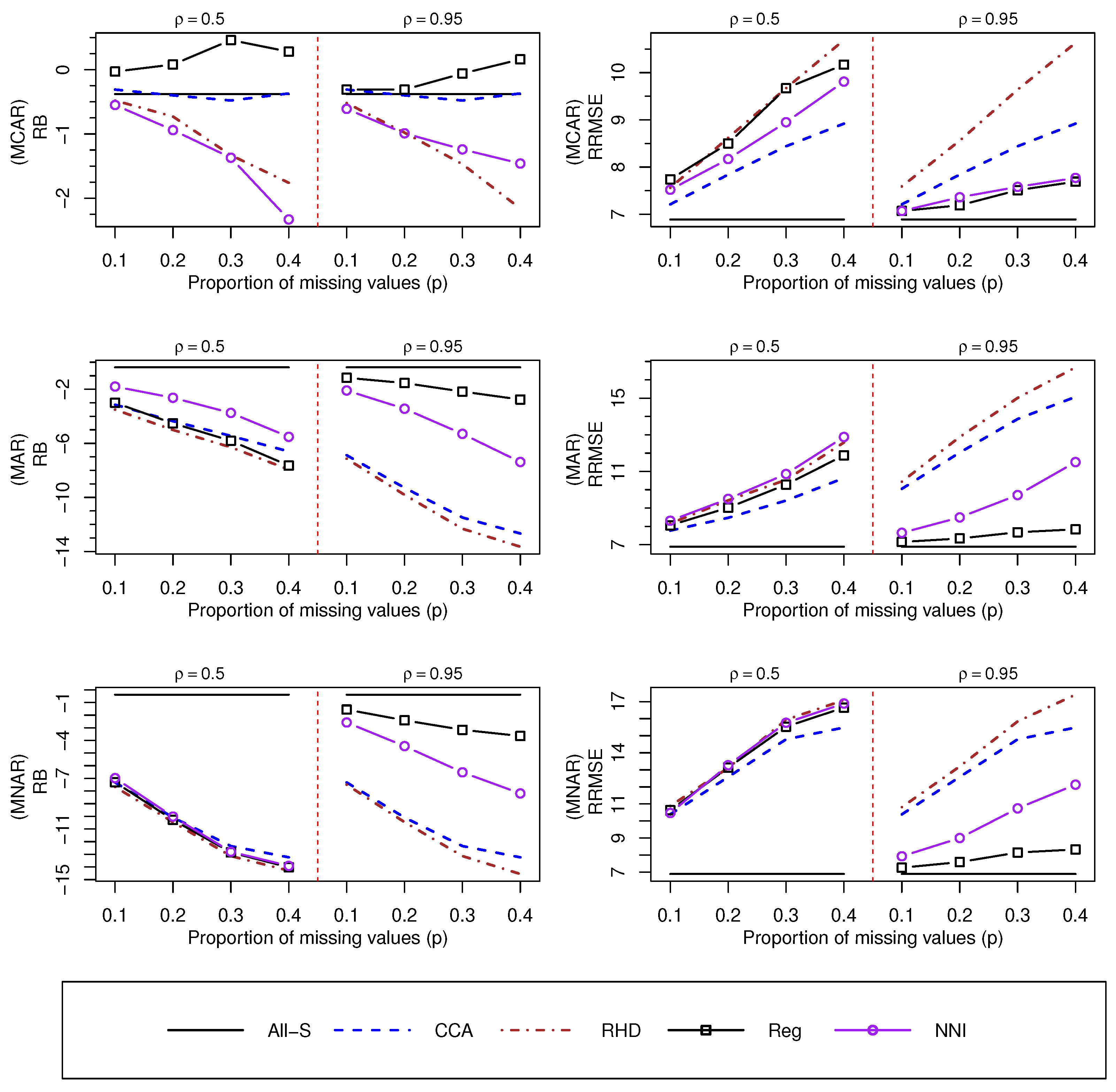
Results from the various Monte Carlo simulation studies can be seen in Figure 1, Figure 2, Figure 3, Figure 4, Figure 5, Figure 6, Figure 7 and Figure 8. Values of and can be seen in Figure 1 and Figure 2 when the true Gini index is given by , respectively.
For a low Gini index (Figure 1), we observe that and yield satisfactory values for under an mechanism and for the various values of p. However, for and mechanisms, values of for the approach decrease as the values of p increase. and methods produce serious biases for the various non-response mechanisms. However, the empirical performance of improves as the value of increases. As expected, and perform better than and in terms of when is large, and the method provides smaller values of , in absolute terms, than the method. The various methods show poor empirical performance when is small and under an mechanism. In summary and as expected, the non-response bias is not a serious issue under an mechanism, although and methods may provide slightly biased estimates. For the mechanism, the various imputation methods give values close to when the proportion of missing data is , and empirical biases increase, in absolute terms, as p increases, so the non-response bias may be non-negligible for large proportions of missing data. Finally, biases based on the mechanism are larger, in absolute terms, that those obtained from an mechanism, so the non-response bias may be a serious issue in this situation.
We may reach some different conclusions, in terms of bias, when G is large (see Figure 2). For instance, the biases of and seem to be affected by p when the assumption holds, since the values of decrease substantially when . In addition, the method shows the worst empirical performance in comparison to alternative approaches when and under a mechanism. Finally, note that the values when are slightly smaller, in absolute terms, than those recorded when . In summary, our results indicate that the non-response bias problem may get worse as the Gini index increases.
As far as the empirical efficiency is concerned, for a low Gini index (see Figure 1), we observe that the various approaches give similar values of when , although the approach is slightly better than alternative methods. However, and provide more efficient results than and when is large, and the method is better than , especially under and mechanisms. Similar conclusions, in terms of , are reached when (see Figure 2).
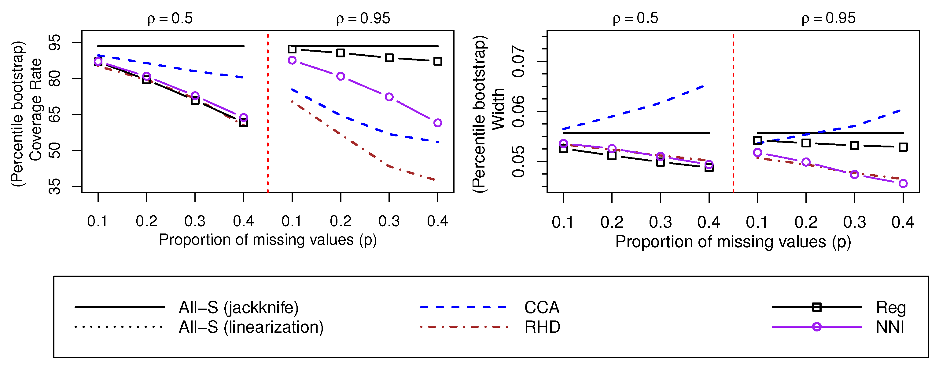
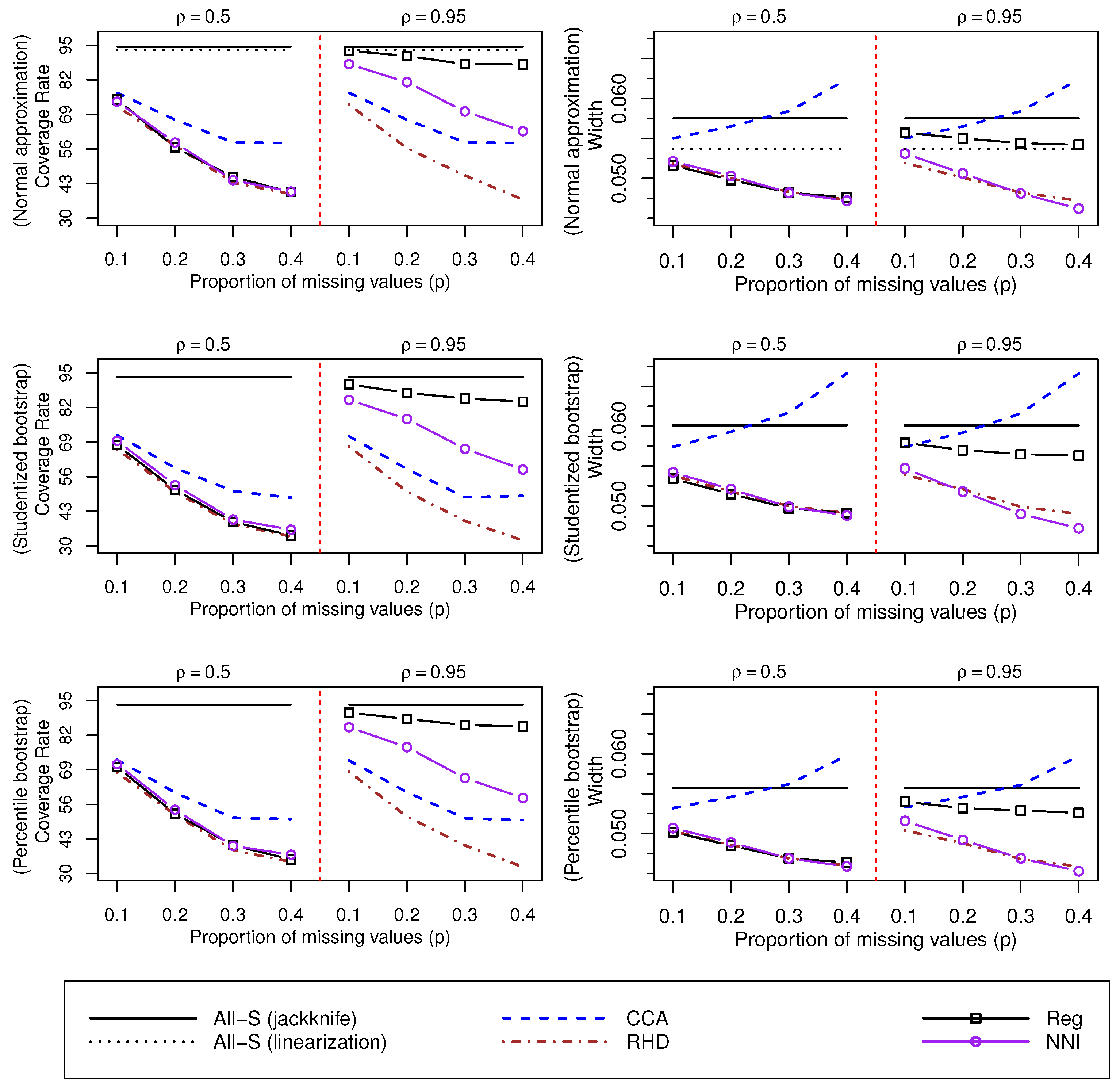
Confidence intervals for are empirically investigated in Figure 3, Figure 4 and Figure 5, which consider the , and mechanisms, respectively. First, we observe that the jackknife variance estimator performs slightly better (in terms of ) than the linearization variance estimator (see, in Figure 3, confidence intervals based on the normal approximation), and for this reason, the various confidence intervals in this study are based on the jackknife variance estimator.
For the mechanism (Figure 3), provides satisfactory empirical coverage rates, but the confidence intervals widen considerably as the proportion of missing data increases. Alternative methods perform poorly in terms of when , although the and imputation methods also give reasonable coverage rates when , and satisfactory values of W for the various values of p. The various methods for the construction of confidence intervals (normal approximation, studentized bootstrap and percentile bootstrap) give similar results. However, confidence intervals based on the studentized bootstrap are slightly wider than confidence intervals based on alternative methodologies (normal approximation and percentile bootstrap).
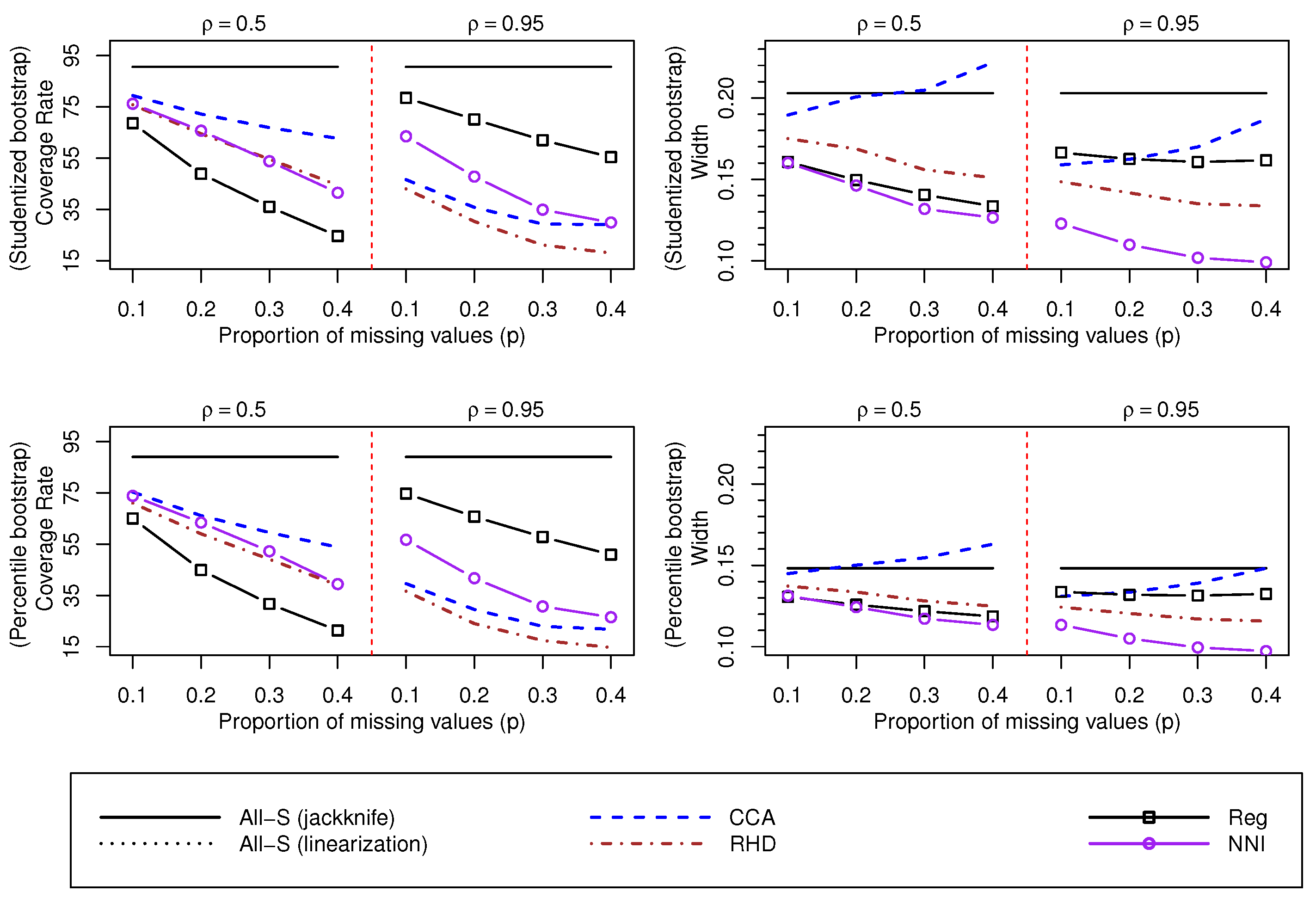
For the mechanism (Figure 4), also provides unsatisfactory coverage rates as p increases. When is large, the best results, in terms of , are obtained using the imputation method, while the imputation method shows the worst performance. As expected, a strong correlation provides better coverage rates with imputation methods based on auxiliary variables ( and ). Note that the bias observed for the mechanism has an impact on the coverage rates of confidence intervals. In particular, values of under the mechanism (Figure 5) are smaller than the corresponding coverage rates under the mechanism (Figure 4).
Finally, results from confidence intervals for can be seen in Figure 6, Figure 7 and Figure 8. First, we observe that confidence intervals perform worse when , since the values of are closer to the required nominal level (95%) when . This is probably due to the fact that estimates of G are slightly more biased when . Again, the imputation method has the best coverage rates when is large, and the method performs poorly for the various scenarios analysed. For the and mechanisms, the various imputation methods provide unsatisfactory coverage rates when p is large, i.e., the bias observed under such situations has a relevant impact on the coverage rates.
4. Conclusions
The problem of missing data may appear in many real-world applications, and various solutions can be applied to handle this problem. The solution adopted in this paper is to use traditional single imputation methods, since they are simple techniques widely used in many National Statistical Institutes, among other official organisms. The non-response bias is an important issue when dealing with missing data, which requires particular attention, especially when the assumption holds. On the other hand, income inequality is a topic of interest in many economic studies, and the Gini index is probably the most commonly-used indicator to measure this phenomenon. In this paper, we empirically evaluate various traditional single imputation methods when applied to the estimation of G, analysing them for multiple interesting scenarios that may arise in practice. In particular, the empirical performance of the customary estimator of G is analysed, and different methods for the construction of confidence intervals are compared. Low and high income inequalities (), and weak and strong correlation coefficients () are analysed. Finally, results are also presented for the various non-response mechanisms (, and ).
First, we analyse the various non-response mechanisms. For an mechanism, and provide appropriate biases. and may yield slightly biased estimates, but they lie within a reasonable range. As expected, the non-response bias is not a problem in this case. In terms of efficiency, the various approaches give similar results for small proportions of missing data, but the and methods show poor values of when the proportion of missing data is large. The various methods give appropriate coverage rates for a small proportion of missing data. provides satisfactory coverage rates for the various values of p, but the confidence intervals based on widen considerably as the value of p increases. and also yield reasonable values of when is large, while poor coverage rates are provided by the method as the value of p increases. For an mechanism, negligible biases are obtained when p is small, but the non-response bias can be a problem if p is large. The method provides the best results, in terms of both and , when is large. The various methods only give reasonable coverage rates when p is small. The method yields good coverage rates for the various values of p when is large. For an mechanism, the non-response bias is a problem for the various methods and the various values of p. However, the method may produce reasonable biases when is large, with values of that can be smaller than , in absolute terms, when . Reasonable coverage rates are only obtained using the method when is large and p is smaller than 0.2, approximately.
Second, we analyse conclusions in terms of the Gini index G. We find that biases increase slightly, in absolute terms, as the income inequality increases. Consequently, coverage rates of confidence intervals are closer to the required confidence level () as the Gini index decreases. As expected, the confidence intervals also widen as the value of G increases.
Third, we analyse the empirical performance of the various imputation methods according to the various proportions of missing data p. The biases of the and methods are not affected by p when the non-response mechanism is and for low income inequalities. Otherwise, the empirical biases increase, in absolute terms, as the proportion of missing data increases. Similar conclusions are reached in terms of , i.e., the values of p do not have an impact on the coverage rates for the mechanism when G is small and is large. As expected, estimators are less efficient as the values of p increase. For an mechanism, the width of confidence intervals based on the various imputation methods is not affected by the value of p, but the width of confidence intervals based on the method increases considerably as the value of p increases. For the and mechanisms, the width of the various confidence intervals is affected by the value of p, although the effect is not relevant for the method when is large.
Fourth, we analyse conclusions in terms of correlation coefficient . As expected, a larger improves the estimation of the and imputation methods, as they make use of the auxiliary variable at the estimation stage. The method clearly outperforms the method when is large. For a large value of , the method can provide empirical biases within a reasonable range for the various non-response mechanisms. However, with a low value of , the non-response bias is a serious problem because the various imputation methods perform poorly in the presence of an mechanism. In addition, the non-response bias is a problem when p is large and the non-response mechanism is . The conclusions are similar in relation of , i.e., poor coverage rates are observed for a low value of and for the and mechanisms, but the method can provide appropriate values of when is large.
Finally, we briefly describe and compare the empirical performance of the various methods investigated in this paper. can be a solution when the non-response mechanism is and is small, but alternative approaches are preferred otherwise. This finding implies that should rarely be used in practice, since the assumption is often unrealistic.
The traditional method provide poor estimates of the Gini index, even for the mechanism when p is large. Note that alternative and more complex techniques can be used in the imputation process and for the various imputation methods, and may yield better results. For instance, the use of imputation classes is a well-known technique that may improve the accuracy of imputation methods.
The method is a good solution when using auxiliary variables and may mitigate the non-response bias problem better than the method when is not extremely large.
The method outperforms its competitors when is large, registering good results in terms of the various empirical measures analysed in this paper and for the various non-response mechanisms. In particular, with a large value of , the method outperforms its competitors when p is large and for the and mechanisms.
As far as the construction of confidence intervals is concerned, we first find that confidence intervals based on the jackknife variance estimator provide coverage rates that are slightly better than those obtained using the linearization variance estimator. The normal approximation and the percentile bootstrap provide confidence intervals with similar empirical properties, while confidence intervals based on the studentized bootstrap are slightly wider than confidence intervals based on the normal approximation and the percentile bootstrap.
5. Discussion
This paper points to various potential areas for future research. First, serious biases have been detected in this study, and they have an important impact on the coverage of confidence intervals. Therefore, the question of how to reduce these biases is an interesting direction for future research. In particular, the bias corrected estimator is considered, but large biases, in absolute terms, are observed when the Gini index is large. The use of additional bias correction procedures has the potential to be a fruitful contribution that may improve the estimation of the Gini index and the corresponding properties of confidence intervals.
We consider single imputation methods, but multiple imputation is also a popular approach that may offer desirable features when it comes to the estimation of the Gini index. Additional single imputation methods can also be investigated, such as the imputation method (see [54,55]), the algorithm (see [56,57]), and the Forest imputation method (see [58,59]), etc.
Recently, the empirical likelihood approach has been used for the construction of confidence intervals for the Gini index (see [22,23,24]). The analysis of the empirical likelihood methodology when dealing with missing data is also an interesting topic for future research.
This study could also be extended to unequal sampling designs and/or multiple auxiliary variables. In particular, the traditional jackknife technique requires an adjustment for samples with unequal inclusion probabilities, and Campbell’s jackknife (see [19,60]) can be a solution when samples selected under a general sampling design suffer from the problem of missing data.
Note that imputation methods have been evaluated here without using imputation classes, and more efficient results are expected for the various imputation methods when using said technique. Finally, we focus exclusively on the Gini index as the indicator to measure inequality. However, the quintile share ratio is another statistic commonly used to measure inequality. Thus, an interesting avenue for future research would be to analyse the performance of the quintile share ratio when single imputation methods are used and compare it with the results obtained in this paper.
Author Contributions
J.F.M.-R., P.J.M.-F. and E.Á.-V. have collaborated equally in the realization of this work. All authors have read and agreed to the published version of the manuscript.
Funding
This research has been partially supported by the Ministry of Economy, Industry and Competitiveness, the Spanish State Research Agency (SRA) and European Regional Development Fund (ERDF) (project reference ECO2017-86822-R). This research has been partially supported by the Ministry of Economy, Industry and Competitiveness, the Spanish State Research Agency (SRA) and European Regional Development Fund (ERDF) (project reference ECO2017-84138-P).
Institutional Review Board Statement
Not applicable.
Informed Consent Statement
Not applicable.
Data Availability Statement
Not applicable.
Conflicts of Interest
The authors declare no conflict of interest.
Abbreviations
The following abbreviations are used in this manuscript:
| MCAR | Missing Completely At Random |
| MAR | Missing At Random |
| MNAR | Missing Not At Random |
| SRSWOR | Simple Random Sampling Without Replacement |
| All-S | All units in the sample S |
| CCA | Complete Case Analysis |
| RHD | Random Hot Desk imputation method |
| Reg | Regression imputation method |
| NNI | Nearest Neighbour Imputation method |
| RB | Relative Bias |
| RRMSE | Relative Root Mean Square Error |
| CR | Coverage Rate |
| W | Width |
References
- Haziza, D.; Lesage, É. A discussion of weighting procedures for unit nonresponse. J. Off. Stat. 2016, 32, 129–145. [Google Scholar] [CrossRef] [Green Version]
- Van Buuren, S. Flexible Imputation of Missing Data; CRC Press: Boca Raton, FL, USA, 2018. [Google Scholar]
- Rubin, D.B. Inference and missing data. Biometrika 1976, 63, 581–592. [Google Scholar] [CrossRef]
- Haziza, D.; Beaumont, J.F. On the construction of imputation classes in surveys. Int. Stat. Rev. 2007, 75, 25–43. [Google Scholar] [CrossRef]
- Little, R.J.; Rubin, D.B. Statistical Analysis with Missing Data, 3rd ed.; John Wiley & Sons: New York, NY, USA, 2019. [Google Scholar]
- Särndal, C.E.; Swensson, B.; Wretman, J. Model Assisted Survey Sampling; Springer Science & Business Media: Berlin/Heidelberg, Germany, 2003. [Google Scholar]
- Rubin, D.B. Multiple imputation after 18+ years. J. Am. Stat. Assoc. 1996, 91, 473–489. [Google Scholar] [CrossRef]
- Carpenter, J.; Kenward, M. Multiple Imputation and Its Application; John Wiley & Sons: Chichester, UK, 2012. [Google Scholar]
- Allison, R.A.; Foster, J.E. Measuring health inequality using qualitative data. J. Health Econ. 2004, 6, 505–524. [Google Scholar] [CrossRef] [PubMed]
- Boyce, J.K.; Zwickl, K.; Ash, M. Measuring environmental inequality. Ecol Econ. 2016, 124, 114–123. [Google Scholar] [CrossRef] [Green Version]
- Ferreira, F.H.; Gignoux, J. The measurement of educational inequality: Achievement and opportunity. World Bank Econ. Rev. 2014, 28, 210–246. [Google Scholar] [CrossRef] [Green Version]
- Solt, F. Measuring income inequality across countries and over time: The standardized world income inequality database. Soc. Sci. Q. 2020, 101, 1183–1199. [Google Scholar] [CrossRef]
- Ravallion, M. Income inequality in the developing world. Science 2014, 344, 851–855. [Google Scholar] [CrossRef]
- Gini, C. Variabilità e mutabilità. Reprinted in Memorie di Metodologica Statistica; Pizetti, E., Ed.; Libreria Eredi Virgilio Veschi: Rome, Italy, 1912. [Google Scholar]
- Kendall, M.; Stuart, A. The Advanced Theory of Statistics: Vol. 1. Distribution Theory, 4th ed.; Charles Griffin: London, UK, 1977. [Google Scholar]
- Lerman, R.I.; Yitzhaki, S. A note on the calculation and interpretation of the Gini index. Econ. Lett. 1984, 15, 363–368. [Google Scholar] [CrossRef]
- Deltas, G. The small-sample bias of the Gini coefficient: Results and implications for empirical research. Rev. Econ. Stat. 1979, 44, 870–872. [Google Scholar]
- Davidson, R. Reliable inference for the Gini index. J. Econom. 2009, 150, 30–40. [Google Scholar] [CrossRef] [Green Version]
- Berger, Y.G. A note on the asymptotic equivalence of jackknife and linearization variance estimation for the Gini coefficient. J. Off. Stat. 2008, 24, 541–555. [Google Scholar]
- Deville, J.C. Variance estimation for complex statistics and estimators: Linearization and residual techniques. Surv. Methodol. 1999, 25, 193–204. [Google Scholar]
- Langel, M.; Tillé, Y. Variance estimation of the Gini index: Revisiting a result several times published. J. R. Stat. Soc. A Stat. Soc. 2013, 176, 521–540. [Google Scholar] [CrossRef] [Green Version]
- Qin, Y.; Rao, J.; Wu, C. Empirical likelihood confidence intervals for the gini measure of income inequality. Econ. Modllng. 2010, 27, 1429–1435. [Google Scholar] [CrossRef] [Green Version]
- Wang, D.; Zhao, Y.; Gilmore, D.W. Jackknife empirical likelihood confidence interval for the Gini index. Stat. Probab. Lett. 2016, 110, 289–295. [Google Scholar] [CrossRef] [Green Version]
- Berger, Y.; Gedik Balay, İ. Confidence intervals of Gini coefficient under unequal probability sampling. J. Off. Stat. 2020, 36, 237–249. [Google Scholar] [CrossRef]
- Giorgi, G.M.; Gigliarano, C. The Gini concentration index: A review of the inference literature. J. Econ. Surv. 2017, 31, 1130–1148. [Google Scholar] [CrossRef]
- Balaji, H.; Mahmoud, H. The Gini index of random trees with an application to caterpillars. J. Appl. Probab. 2017, 54, 701–709. [Google Scholar] [CrossRef]
- Ren, Y.; Zhang, P.; Dey, D.K. Investigating Several Fundamental Properties of Random Lobster Trees and Random Spider Trees. Methodol. Comput. Appl. Probab. 2021, 1–17. [Google Scholar] [CrossRef]
- Parsa, M.; Di Crescenzo, A.; Jabbari, H. Analysis of reliability systems via Gini-type index. Eur. J. Oper. Res. 2018, 264, 340–353. [Google Scholar] [CrossRef]
- Ma, J. Generalised grey target decision method for mixed attributes based on the improved Gini–Simpson index. Soft Comput. 2018, 23, 13449–13458. [Google Scholar] [CrossRef]
- Atkinson, A.B. On the measurement of inequality. J. Econ. Theory 1970, 2, 244–263. [Google Scholar] [CrossRef]
- Evans, M.D.; Kelley, J.; Kelley, S.M.; Kelley, C.G. Rising Income Inequality During the Great Recession Had No Impact on Subjective Wellbeing in Europe, 2003–2012. J. Happiness Stud. 2019, 20, 203–228. [Google Scholar] [CrossRef]
- Detollenaere, J.; Desmarest, A.S.; Boeckxstaens, P.; Willems, S. The link between income inequality and health in Europe, adding strength dimensions of primary care to the equation. Soc. Sci. Med. 2018, 201, 103–110. [Google Scholar] [CrossRef] [PubMed]
- Zagorski, K.; Evans, M.D.; Kelley, J.; Piotrowska, K. Does national income inequality affect individuals’ quality of life in Europe? Inequality, happiness, finances, and health. Soc. Indic. Res. 2014, 117, 1089–1110. [Google Scholar] [CrossRef]
- Rueda, M.M.; Muñoz, J.F. Estimation of poverty measures with auxiliary information in sample surveys. Qual. Quant. 2011, 45, 687–700. [Google Scholar] [CrossRef]
- Langel, M.; Tillé, Y. Statistical inference for the quintile share ratio. J. Stat. Plan. Inference 2011, 141, 2976–2985. [Google Scholar] [CrossRef] [Green Version]
- Rao, J.N.K. On variance estimation with imputed survey data. J. Am. Stat. Assoc. 1996, 91, 499–506. [Google Scholar] [CrossRef]
- Zhong, H. The impact of missing data in the estimation of concentration index: A potential source of bias. Eur. Health Econ. 2010, 11, 255–266. [Google Scholar] [CrossRef] [PubMed]
- Chen, Y.; Fu, D. Measuring income inequality using survey data: The case of China. J. Econ. Inequal. 2015, 13, 299–307. [Google Scholar] [CrossRef]
- Ardington, C.; Lam, D.; Leibbrandt, M.; Welch, M. The sensitivity to key data imputations of recent estimates of income poverty and inequality in South Africa. Econ. Model. 2005, 23, 822–835. [Google Scholar] [CrossRef] [Green Version]
- Jenkins, S.P. World income inequality databases: An assessment of WIID and SWIID. J. Econ. Inequal. 2015, 13, 629–671. [Google Scholar] [CrossRef] [Green Version]
- Yitzhaki, S. More than a dozen alternative ways of spelling Gini. Res. Econ. Inequal. 1998, 8, 13–30. [Google Scholar]
- David, H.A. Order Statistics; Wiley: NewYork, NY, USA, 1970. [Google Scholar]
- Ogwang, T. A convenient method of computing the Gini index and its standard error. Oxf. Bull. Econ. Stat. 2000, 62, 123–129. [Google Scholar] [CrossRef]
- Demnati, A.; Rao, J.N.K. Linearization variance estimators for survey data. Surv. Methodol. 2004, 30, 17–26. [Google Scholar]
- Yitzhaki, S. Calculating jackknife variance estimators for parameters of the Gini method. Surv. Methodol. 1991, 9, 235–239. [Google Scholar]
- Karagiannis, E.; Kovačević, M. A method to calculate the jackknife variance estimator for the Gini coefficient. Oxf. Bull. Econ. Stat. 2000, 62, 119–122. [Google Scholar] [CrossRef]
- Kuan, X. Inference for generalized Gini indices using the iterated bootstrap method. J. Bus. Econ. Statist. 2000, 18, 223–227. [Google Scholar]
- Giorgi, G.M.; Palmitesta, P.; Provasi, C. Asymptotic and bootstrap inference for the generalized gini indices. Metron 2006, 64, 107–124. [Google Scholar]
- Muñoz, J.F.; Rueda, M. New imputation methods for missing data using quantiles. J. Comput. Appl. Math. 2009, 232, 305–317. [Google Scholar] [CrossRef]
- Andridge, R.R.; Little, R.J. A review of hot deck imputation for survey non-response. Int. Stat. Rev. 2010, 78, 40–64. [Google Scholar] [CrossRef]
- Healy, M.; Westmacott, M. Missing values in experiments analysed on automatic computers. J. R. Stat. Soc. Ser. C Appl. Stat. 1956, 5, 203–206. [Google Scholar] [CrossRef]
- Chen, J.; Shao, J. Nearest neighbor imputation for survey data. J. Off. Stat. 2000, 16, 113–131. [Google Scholar]
- Gower, J.C. A general coefficient of similarity and some of its properties. Biometrics 1971, 27, 857–871. [Google Scholar] [CrossRef]
- Kim, K.Y.; Kim, B.J.; Yi, G.S. Reuse of imputed data in microarray analysis increases imputation efficiency. BMC Bioinform. 2004, 5, 1–9. [Google Scholar] [CrossRef] [Green Version]
- Moya-Fernández, P.J.; López-Ruiz, S.; Guardiola, J.; González-Gómez, F. Determinants of the acceptance of domestic use of recycled water by use type. Sustain. Prod. Consum. 2021, 27, 575–586. [Google Scholar] [CrossRef]
- McLachlan, G.J.; Krishnan, T. The EM Algorithm and Extensions, 2nd ed.; John Wiley & Sons: New York, NY, USA, 2007. [Google Scholar]
- Lange, K. A gradient algorithm locally equivalent to the EM algorithm. J. R. Stat. Soc. Ser. B Stat. Methodol. 1995, 57, 425–437. [Google Scholar] [CrossRef] [Green Version]
- Pantanowitz, A.; Marwala, T. Missing data imputation through the use of the random forest algorithm. In Advances in Computational Intelligence; Springer: Berlin, Germany, 2009; pp. 53–62. [Google Scholar]
- Tang, F.; Ishwaran, H. Random forest missing data algorithms. Stat. Anal. Data. Min. 2007, 10, 363–377. [Google Scholar] [CrossRef]
- Campbell, N.A. Robust procedures in multivariate analysis I: Robust covariance estimation. J. R. Stat. Soc. Ser. C Appl. Stat. 1980, 29, 231–237. [Google Scholar] [CrossRef]
Figure 1.
Values of and for when estimating .

Figure 2.
Values of and for when estimating .

Figure 3.
Values of and W associated with confidence intervals for , and based on the jackknife variance estimator. The mechanism is considered. Linearization and jackknife variances are compared using the normal approximation and the approach.
Figure 3.
Values of and W associated with confidence intervals for , and based on the jackknife variance estimator. The mechanism is considered. Linearization and jackknife variances are compared using the normal approximation and the approach.

Figure 4.
Values of and W associated with confidence intervals for , and based on the jackknife variance estimator. The mechanism is considered. Linearization and jackknife variances are compared using the normal approximation and the approach.
Figure 4.
Values of and W associated with confidence intervals for , and based on the jackknife variance estimator. The mechanism is considered. Linearization and jackknife variances are compared using the normal approximation and the approach.


Figure 5.
Values of and W associated to confidence intervals for , and based on the jackknife variance estimator. The mechanism is considered. Linearization and jackknife variances are compared using the normal approximation and the approach.
Figure 5.
Values of and W associated to confidence intervals for , and based on the jackknife variance estimator. The mechanism is considered. Linearization and jackknife variances are compared using the normal approximation and the approach.

Figure 6.
Values of and W associated to confidence intervals for , and based on the jackknife variance estimator. The mechanism is considered. Linearization and jackknife variances are compared using the normal approximation and the approach.
Figure 6.
Values of and W associated to confidence intervals for , and based on the jackknife variance estimator. The mechanism is considered. Linearization and jackknife variances are compared using the normal approximation and the approach.

Figure 7.
Values of and W associated to confidence intervals for , and based on the jackknife variance estimator. The mechanism is considered. Linearization and jackknife variances are compared using the normal approximation and the approach.
Figure 7.
Values of and W associated to confidence intervals for , and based on the jackknife variance estimator. The mechanism is considered. Linearization and jackknife variances are compared using the normal approximation and the approach.


Figure 8.
Values of and W associated to confidence intervals for , and based on the jackknife variance estimator. The mechanism is considered. Linearization and jackknife variances are compared using the normal approximation and the approach.
Figure 8.
Values of and W associated to confidence intervals for , and based on the jackknife variance estimator. The mechanism is considered. Linearization and jackknife variances are compared using the normal approximation and the approach.

Publisher’s Note: MDPI stays neutral with regard to jurisdictional claims in published maps and institutional affiliations. |
© 2021 by the authors. Licensee MDPI, Basel, Switzerland. This article is an open access article distributed under the terms and conditions of the Creative Commons Attribution (CC BY) license (https://creativecommons.org/licenses/by/4.0/).
Share and Cite
MDPI and ACS Style
Álvarez-Verdejo, E.; Moya-Fernández, P.J.; Muñoz-Rosas, J.F. Single Imputation Methods and Confidence Intervals for the Gini Index. Mathematics 2021, 9, 3252. https://0-doi-org.brum.beds.ac.uk/10.3390/math9243252
AMA Style
Álvarez-Verdejo E, Moya-Fernández PJ, Muñoz-Rosas JF. Single Imputation Methods and Confidence Intervals for the Gini Index. Mathematics. 2021; 9(24):3252. https://0-doi-org.brum.beds.ac.uk/10.3390/math9243252
Chicago/Turabian StyleÁlvarez-Verdejo, Encarnación, Pablo J. Moya-Fernández, and Juan F. Muñoz-Rosas. 2021. "Single Imputation Methods and Confidence Intervals for the Gini Index" Mathematics 9, no. 24: 3252. https://0-doi-org.brum.beds.ac.uk/10.3390/math9243252
Note that from the first issue of 2016, this journal uses article numbers instead of page numbers. See further details here.