Hypergraph-Supervised Deep Subspace Clustering

Abstract

Auto-encoder (AE)-based deep subspace clustering (DSC) methods aim to partition high-dimensional data into underlying clusters, where each cluster corresponds to a subspace. As a standard module in current AE-based DSC, the self-reconstruction cost plays an essential role in regularizing the feature learning. However, the self-reconstruction adversely affects the discriminative feature learning of AE, thereby hampering the downstream subspace clustering. To address this issue, we propose a hypergraph-supervised reconstruction to replace the self-reconstruction. Specifically, instead of enforcing the decoder in the AE to merely reconstruct samples themselves, the hypergraph-supervised reconstruction encourages reconstructing samples according to their high-order neighborhood relations. By the back-propagation training, the hypergraph-supervised reconstruction cost enables the deep AE to capture the high-order structure information among samples, facilitating the discriminative feature learning and, thus, alleviating the adverse effect of the self-reconstruction cost. Compared to current DSC methods, relying on the self-reconstruction, our method has achieved consistent performance improvement on benchmark high-dimensional datasets.

1. Introduction

Subspace clustering has drawn increasing attention in computational intelligence and data mining [1,2]. By assuming high-dimensional data resides in a set of low-dimensional linear subspaces, numerous pioneer subspace clustering methods [3,4,5,6] aim to segment the data into their corresponding subspaces. Most of these approaches exploit the self-expression formulation. That is, each data sample can be expressed as a linear combination of other samples, and the combination coefficients indicate the respective subspaces. Over the last decade, this line of methods has witnessed their success in plenty of scientific fields [7], such as computer vision [8]. Nevertheless, in practical situations, the data do not necessarily accord with linear subspace models, as shown in [9], and the applicability of such linear models are, thus, limited.

Rising to this challenge, DSC [9,10] provides a powerful framework to perform nonlinear feature learning, collaboratively with deep neural networks and subspace clustering. In DSC, a standard neural network is the deep AE [11], which mainly involves an encoder and decoder. The former performs deep feature learning by mapping the original features of samples into a latent space (the output of the encoder is referred to as the latent representation). Taking the outputs of the encoder as input, the decoder attempts to map them back to the original space by the guidance of the self-reconstruction cost function. For example, Peng et al. [12] applied a deep AE with a sparse prior [4], in which they conduct sparse subspace clustering on the latent representation of the deep AE. Later, Peng et al. [10] came up with the DSC with ${\ell }_1$-norm (DSC-L1), which imposes the sparsity to the latent representation of a deep AE. Ji et al. [9] presented the DSC networks (DSC-Nets) using deep AE, introducing a novel self-expression layer at the junction between the encoder and decoder. The self-expression layer seamlessly combines deep feature learning and subspace clustering.

Recently, a few studies have attempted to exploit pseudo-labels to guide the neural networks for deep discriminative feature learning. Since the DSC involves both the deep neural network and clustering, a natural idea is to use the pseudo-labels, extracted from the self-expression layer, to help discriminative the feature learning of neural networks. Zhang et al. [13] proposed a self-supervised convolutional subspace clustering network (S${}^2$ ConvSCN) that enhances the deep discriminative feature with pseudo-labels. In particular, they insert a fully-connected (FC) layer, coupled with a softmax function after the encoder. Then, they perform pseudo-label training with a mixture of the cross-entropy and center cost.

Although DSC has been substantially developed, a potential issue is that the self-reconstruction cost used in most DSC methods can negatively affect the discriminative feature learning of the encoder. In principle, the self-reconstruction cost exists to regularize the deep feature learning of the encoder, e.g., preventing the latent representation of the samples from collapsing into a single point [14]. However, it is shown that self-reconstruction cost over-regularizes the deep AE and degrades the discriminability of the latent representation of the encoder [15,16].

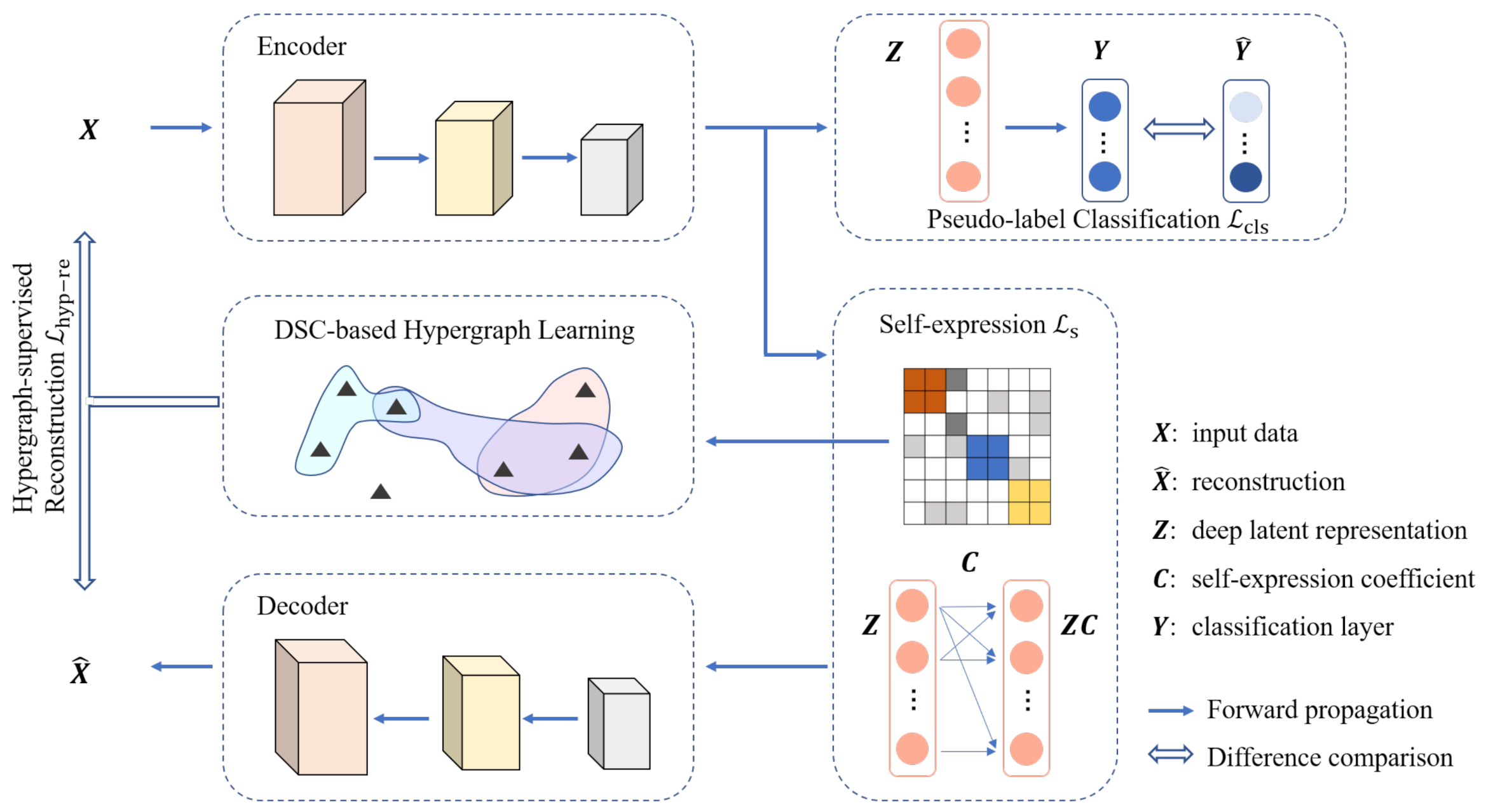
To address this issue, this paper proposes a hypergraph-supervised deep subspace clustering method (H-DSC), as shown in Figure 1. Similar to [13,17], we employ the standard AE as the deep feature extractor, with the self-expression module in between. We also introduce a classification module, attached to the encoder, which enables the supervision of the pseudo-labels. Differently, we apply a hypergraph to reform the self-reconstruction cost. The over-regularization of the self-reconstruction partly stems from the fact that it simply enforces the decoder to reconstruct the samples themselves and neglects the informative sample relations [16,18]. Such a self-reconstruction cost undermines the discriminability of the deep AE, when trained by a standard back-propagation algorithm. Intuitively, samples have different importance in the reconstruction, to reflect their individual roles. To this end, we formulate the hypergraph-supervised reconstruction cost, which encourages the decoder to reconstruct samples, based on the high-order relations in the hypergraph [19]. A hypergraph is a generalization of a graph, in which a hyperedge can connect an arbitrary number of vertices or samples. This property endows a hypergraph to characterize the high-order relations among samples and can be exploited to facilitate the deep feature learning. Through back-propagation training, this hypergraph-supervised cost function allows the encoder to capture high-order neighborhood structure information [20]. In this sense, the hypergraph-supervised reconstruction cost enhances the discriminative feature learning of the encoder and mitigates the adverse effect of the self-reconstruction, leading to an improved clustering performance. Empirical evaluations on benchmark high-dimensional datasets have shown that our method consistently outperforms current DSC methods with the self-reconstruction.

The contribution of this paper is summarized as follows.

• We propose a hypergraph-supervised DSC that alleviates the adverse effect of the self-reconstruction cost, improving the clustering performance.
• We propose a hypergraph learning, based on the rich information from the self-expression layer, enabling the hypergraph and DSC to collaborate and improve the clustering performance.
• We conduct experiments, including a series of ablation studies on benchmark high-dimensional datasets, to illustrate the effectiveness of our proposed method.

2. Related Work

2.1. Subspace Clustering

Let $\mathit{X}=[{\mathit{x}}_1,{\mathit{x}}_2,\cdots ,{\mathit{x}}_m]\in {\mathbb{R}}^{n_x\times m}$ be a data matrix, with m samples and $n_x$ dimension. The overarching goal of subspace clustering is to group the samples into respective clusters, where a cluster corresponds to a subspace. Most early works in subspace clustering [3,4,5,6] attempt leverage the self-expression, to identify which subspaces the given samples belong to. Formally, the self-expression can be written via the following:

$$\begin{array}{c}\hfill \underset{\mathit{C}}{min}\frac{1}{2}\left|\right|\mathit{X}-{\mathit{X}\mathit{C}\left|\right|}_F^2+{\sigma \left|\right|\mathit{C}\left|\right|}_p,\end{array}$$

(1)

where $\sigma$ is a trade-off parameter, and the coefficient matrix $\mathit{C}\in {\mathbb{R}}^{m\times m}$ indicates sample affinities. For example, if ${\mathit{x}}_i$ and ${\mathit{x}}_j$ belong to the same subspace, then ${\mathit{C}}_{ij}$ and ${\mathit{C}}_{ji}$ tend to be large. In contrast, if ${\mathit{x}}_i$ and ${\mathit{x}}_k$ belong to the different subspaces, then ${\mathit{C}}_{ik}$ and ${\mathit{C}}_{ki}$ tend to be small. Here, ${\left|\right|\mathit{C}\left|\right|}_p$ denotes the prior term to prevent trivial solutions [6]. For instance, the sparsity term ${\left|\right|\mathit{C}\left|\right|}_1$ [3,4], nuclear norm or low-rank term ${\left|\right|\mathit{C}\left|\right|}_{*}$ [5], and dense term or F-norm [6]. After obtaining $\mathit{C}$, those methods often conduct spectral clustering [21] on the similarity matrix $\mathit{S}=\frac{1}{2}\left(\right|\mathit{C}|+{\left|\mathit{C}\right|}^{\top })$ to finally cluster the samples.

2.2. Deep Subspace Clustering

The main challenge of these traditional subspace clustering methods is that they are limited to apply to the linear subspace cases [9]. To address this issue, some kernel based subspace clustering methods [22] have been proposed, yet it remains hard to choose proper kernels for the underlying subspaces [9]. Recently, deep subspace clustering methods [9,12,23] have provided a promising direction, and they leverage deep neural networks to perform nonlinear feature learning and subspace clustering collaboratively. Most deep subspace clustering methods follow the pattern from [9]. Formally, the deep encoder $f_E(;{\Theta }_e):{\mathbb{R}}^{n_x}\to {\mathbb{R}}^{n_z}$ is employed to map the original sample ${\mathit{x}}_i$ for $i\in \left[m\right]$ to the latent space: ${\mathit{z}}_i=f_E({\mathit{x}}_i;{\Theta }_e)$, where ${\Theta }_e$ and $n_z$ stand for the parameter of the encoder and dimension of the latent presentation ${\mathit{z}}_i$, respectively. Afterward, a decoder $f_D(;{\Theta }_d):{\mathbb{R}}^{n_z}\to {\mathbb{R}}^{n_x}$ is adopted to regularize the encoder [14] by mapping the latent representation ${\mathit{z}}_i$ for $i\in \left[m\right]$ back to the original space, denoted by ${\widehat{\mathit{x}}}_i$, where ${\Theta }_d$ denotes the parameter of the decoder. The self-expression is then performed in the latent space $\mathit{Z}$. Combining the deep AE reconstruction and self-expression, they have the following formulation:

$$\begin{array}{c}\hfill \underset{{\Theta }_e,{\Theta }_d,\mathit{C}}{min}{\mathcal{L}}_{\mathrm{self}-\mathrm{re}}+{\beta }_1{\mathcal{L}}_{\mathrm{s}},\end{array}$$

(2)

where ${\mathcal{L}}_{\mathrm{self}-\mathrm{re}}={\sum }_{i,j}\left|\right|{\mathit{x}}_i-{\widehat{\mathit{x}}}_j{\left|\right|}_2^2=\left|\right|\mathit{X}-\widehat{\mathit{X}}{\left|\right|}_F^2$, ${\mathcal{L}}_{\mathrm{s}}=\left|\right|\mathit{Z}-{\mathit{Z}\mathit{C}\left|\right|}_F^2+{\sigma \left|\right|\mathit{C}\left|\right|}_F$, and $\mathit{Z}$ denotes the latent representation matrix whose columns are ${\mathit{Z}}_i$ for $i\in \left[m\right]$. The ${\mathcal{L}}_{\mathrm{self}-\mathrm{re}}$ is the self-reconstruction term, and ${\mathcal{L}}_{\mathrm{s}}$ is the self-expression in $\mathit{Z}$. F-norm on $\mathit{C}$ is adopted for ease of follow-up gradient-based training. Again, ${\beta }_1$ is a trade-off parameter. Notably, Ji et al. [9] added a fully-connected layer, without a bias between the encoder and decoder, whose weights represent the coefficient matrix $\mathit{C}$; they call it the self-expression layer. Thereafter, several works have been proposed. Peng et al. [23] combined a structured AE-based DSC with linear subspace clustering. By incorporating adversarial training into DSC, some studies observed the improvement of clustering [24]. Jiang et al. [25] incorporated the self-paced technique into DSC to gradually improve the clustering ability. Recently, Peng et al. [10] came up with DSC-L1, with the sparsity on the latent representation. Multiple linear layers have been exploited to characterize the low- and high-level information for DSC [26].

More recently, Zhang et al. [13] introduced the classification module that can leverage the pseudo-labels extracted from the self-expression layer. Xu et al. [27] proposed a DSC method that jointly learns an AE and latent block-diagonal representation matrix. ODSC is proposed to leverage overcomplete representation for robust clustering [28]. Differently, Peng et al. [29] proposed a DSC method with the maximum entropy term that increases the connectivity of the learned affinity matrix. Building upon the idea of data augmentation, Abavisani et al. [8] came up with a temporal ensembling component that enables the DSC to maintain invariant subspaces from random data transformations.

However, the above methods share a common challenge: they mostly employ the self-reconstruction cost in their frameworks, limiting the deep feature learning of the encoder. Some recent studies [14,15,17] attempt to address this issue. A typical example is the locality preserving module for reconstruction, proposed by [17]. Nevertheless, we find that the locality preserving module amounts to a graph regularization, which merely depicts the pairwise relations of samples. Unlike [17], we propose a hypergraph-supervised reconstruction that exploits the high-order relations among samples, enhancing the deep discriminative feature learning of the encoder and improving the clustering performance.

3. Method

This section formally presents our proposed hypergraph-supervised deep subspace clustering (H-DSC) method, as shown in Figure 1. We first present background information, regarding hypergraphs; then, we detail our framework, which mainly consists of two parts: (1) hypergraph-supervised AE with the self-expression layer to perform the deep feature learning and subspace clustering collaboratively; (2) the classification module that enables supervision from the pseudo-labels. These two parts are seamlessly connected and mutually enhance each other. The notation used in this article is summarized in

Table 1. The definitions of notations.

Notation	Remark
$\mathit{X}$	Data matrix
$\mathit{Z}$	Deep latent representation
${\mathit{x}}_i$/${\mathit{z}}_i$	The i-th sample in $\mathit{X}$/$\mathit{Z}$
$\mathit{C}$	Self-expression coefficient matrix
$\mathit{S}$	Similarity matrix formed by $\mathit{C}$
$\mathit{H}$	Incidence matrix of hypergraph
${\mathit{D}}_v$	Degree matrix of vertices in hypergraph
${\mathit{D}}_e$	Degree matrix of hyperedges
$\mathit{W}$	Weight matrix of hyperedges
${\mathit{L}}_h$	Hypergraph Laplacian matrix
${\mathit{y}}_i$	The i-th sample in classification layer
${\widehat{\mathit{y}}}_i$	Pseudo-label for i-th sample
m	Number of samples
K	Number of clusters
$\left[m\right]$	The set of $\{1,2,\cdots ,m\}$

for ease of exposition.

3.1. Preliminaries on Hypergraphs

The hypergraphs are a generalization of graphs [19], providing a natural way to characterize the high-order relations among samples. A standard hypergraph, and its Laplacian, are proposed by Zhou, Huang, and Scholköpf [30], who generalized the regularized graphs and define the normalized hypergraph Laplacian. Formally, given a hypergraph $\mathbb{G}=(\mathbb{V},\mathbb{E},\mathit{W})$, with $\mathbb{V}$, $\mathbb{E}$, and $\mathit{W}$ denoting the sample (vertex) set, the hyperedge set, and the weight matrix, respectively. Denote the weight corresponding to the hyperedge $e_j$ as $\omega \left(e_j\right)$. The degree of a vertex $a_i$ is defined as $d\left(a_i\right)={\sum }_{e_j\in \mathbb{E},a_i\in e_j}\omega \left(e_j\right)$. The incidence matrix $\mathit{H}\in {\mathbb{R}}^{\left|\mathbb{V}\right|\times \left|\mathbb{E}\right|}$ is constructed to indicate the association between samples and hyperedges, i.e., the entry ${\mathit{H}}_{i,j}\triangleq h(a_i,e_j)=1$ if $a_i\in e_j$ and entry ${\mathit{H}}_{i,j}\triangleq h(a_i,e_j)=0$ otherwise. The degree of the hyperedge $e_j$ is $\delta \left(e_j\right)=\left|e_j\right|$. By definitions, we have:

$$\begin{array}{c}\hfill d\left(a_i\right)=\sum _{e_j\in \mathbb{E}}\omega \left(e_j\right)h(a_i,e_j)\mathrm{and}\delta \left(e_j\right)=\sum _{a_i\in \mathbb{V}}h(a_i,e_j).\end{array}$$

(3)

To use a concise matrix form, we denote the diagonal matrix ${\mathit{D}}_V$ and ${\mathit{D}}_E$ as the degree matrix of the vertex and hyperedge, whose elements are ${\left({\mathit{D}}_V\right)}_{i,i}=d\left(a_i\right)$ and ${\left({\mathit{D}}_E\right)}_{j,j}=\delta \left(e_j\right)$. The hyperedge weight matrix can be a diagonal matrix, whose element is ${\mathit{W}}_{j,j}=\omega \left(e_j\right)$. The hypergraph Laplacian is then defined as [30]:

$$\begin{array}{c}\hfill {\mathit{L}}_h=\mathit{I}-{{\mathit{D}}_V}^{-1/2}\mathit{H}\mathit{W}{{\mathit{D}}_E}^{-1}{\mathit{H}}^{\top }{{\mathit{D}}_V}^{-1/2}.\end{array}$$

(4)

The hypergraph, along with its Laplacian, has demonstrated its effectiveness as a regularization for various learning problems, owing to the powerful representation of high-order relations [31,32]. In this paper, we leverage the powerful representation of the hypergraph, to help improve the DSC by formulating a hypergraph-supervised reconstruction, which specifically enhances the encoder to discover the high-order relations of samples and facilitate the clustering.

3.2. Hypergraph-Supervised Auto-Encoder

Let $\mathit{X}=[{\mathit{x}}_1,{\mathit{x}}_2,\cdots ,{\mathit{x}}_m]\in {\mathbb{R}}^{n_x\times m}$ be a data matrix, with m samples, which lie in a union of low-dimensional subspaces of ${\mathbb{R}}^{n_x}$. Similar to the standard deep subspace clustering mentioned in Section 2.2, we employ the deep encoder, $f_E(;{\Theta }_e):{\mathbb{R}}^{n_x}\to {\mathbb{R}}^{n_z}$, that maps the original sample ${\mathit{x}}_i$ for $i\in \left[m\right]$ to the latent space: ${\mathit{z}}_i=f_E({\mathit{x}}_i;{\Theta }_e)$, as well as a decoder $f_D(;{\Theta }_d):{\mathbb{R}}^{n_z}\to {\mathbb{R}}^{n_x}$ to regularize the encoder [14] by mapping the latent representation ${\mathit{z}}_i$ for $i\in \left[m\right]$ back to the original space, denoted by ${\widehat{\mathit{x}}}_i$. Differently, we have no longer applied the self-reconstruction in Equation (2).

Hypergraph-supervised Reconstruction. Most DSC methods [9,10,12] employ the self-reconstruction that serves as a necessary regularization to the deep AE [14]. Nevertheless, the potential issue is that the self-reconstruction often over-regularizes the encoder and hampers the deep feature learning [15,16], when the deep AE are trained by the back-propagation. A possible remedy for this issue is the locality preservation module [17], which attempts to reconstruct the neighbors of given samples, rather than themselves. Formally, ${\mathit{x}}_i$ is encouraged to reconstruct its neighbor ${\mathit{x}}_j$, with the weight ${\mathit{S}}_{i,j}$, where ${\mathit{S}}_{i,j}$, obtained by the self-expression layer, represents the affinity between samples ${\mathit{x}}_i$ and ${\mathit{x}}_j$. The basic idea is that samples with higher affinities should be similar in reconstruction. Then, the corresponding graph-regularized reconstruction comes out as:

$$\begin{array}{c}\hfill \underset{{\Theta }_e,{\Theta }_d}{min}\sum _{i,j}{\mathit{S}}_{i,j}\left|\right|{\mathit{x}}_i-{\widehat{\mathit{x}}}_j{\left|\right|}_2^2=\left|\right|\mathit{X}-\widehat{\mathit{X}}{\left|\right|}_F^2+2Tr\left(\mathit{X}\mathit{L}{\widehat{\mathit{X}}}^{\top }\right),\end{array}$$

(5)

where the normalized Laplacian matrix $\mathit{L}=\mathit{I}-{\mathit{D}}^{-\frac{1}{2}}\mathit{S}{\mathit{D}}^{-\frac{1}{2}}$, the diagonal matrix $\mathit{D}=\mathrm{Diag}\left({\sum }_{j=1}^m{\mathit{S}}_{i,j}\right)$, and $Tr\left(\right)$ denote the trace operation.

However, we note that the weighted reconstruction in Equation (5) amounts to a pairwise graph regularization, which is limited to depict the pairwise relations of samples [20]. To address this issue, we propose hypergraph-supervised reconstruction, which allows the deep AE to characterize high-order relations. Formally, suppose we are given a hypergraph $\mathbb{G}=(\mathbb{V},\mathbb{E},\mathit{W})$, as mentioned in Section 3.1, where a vertex corresponds to a sample in $\mathit{X}$. The hypergraph reconstruction will be discussed later. Intuitively, we hypothesize that the samples within the same hyperedge e are similar to each other in the reconstruction. We then encourage the samples within the same hyperedge to be decoded through a weighting, based on $\frac{\omega \left(e\right)}{\delta \left(e\right)}$. Accordingly, we formulate the hypergraph-supervised reconstruction as:

$$\begin{array}{c}\hfill \underset{{\Theta }_e,{\Theta }_d}{min}\sum _{e\in \mathbb{E}}\sum _{({\mathit{x}}_i,{\mathit{x}}_j)\in e}\frac{\omega \left(e\right)}{\delta \left(e\right)}\left|\right|{\mathit{x}}_i-{\widehat{\mathit{x}}}_j{\left|\right|}_2^2.\end{array}$$

(6)

This formulation makes the samples within the same hyperedge decode similarly. In other words, the high-order relations among these samples are reflected in the reconstruction. By the subsequent back-propagation training, the hypergraph-supervised reconstruction in Equation (6) enables the deep AE to perform a more discriminative feature learning, compared to the graph-regularized reconstruction and, thus improves clustering performance. After the algebraic manipulations, according to [20], we can derive the matrix form, as follows:

$$\begin{array}{cc}\hfill & {\mathcal{L}}_{\mathrm{hyp}-\mathrm{re}}=\underset{{\Theta }_e,{\Theta }_d}{min}\sum _{e\in \mathbb{E}}\sum _{({\mathit{x}}_i,{\mathit{x}}_j)\in e}\frac{\omega \left(e\right)}{\delta \left(e\right)}\left|\right|{\mathit{x}}_i-{\widehat{\mathit{x}}}_j{\left|\right|}_2^2\hfill \\ \hfill & =\left|\right|\mathit{X}-\widehat{\mathit{X}}{\left|\right|}_F^2+2Tr\left(\mathit{X}{\mathit{L}}_h{\widehat{\mathit{X}}}^{\top }\right),\hfill \end{array}$$

(7)

where ${\mathit{L}}_h$ is exactly the hypergraph Laplacian in Equation (4).

DSC-based Hypergraph Learning. There remains the question of how to construct the hypergraph, i.e., the incidence matrix $\mathit{H}$ and the hyperedge weight matrix $\mathit{W}$. Numerous plausible approaches have been studies in the hypergraph literature [33], but few of them are well connected with the DSC. In this paper, we propose a data-driven approach that learns the hypergraph from the self-expression layer of DSC. Given the data $\mathit{X}$, we assume each sample ${\mathit{x}}_i$ form a vertex of the hypergraph; thus, the incidence matrix $\mathit{H}$ becomes a square matrix, with size $m\times m$. The $\mathit{S}$ formed from the self-expression layer provides rich information about the geometry structure of samples, and such information can be exploited to construct the hypergraph. Intuitively, samples with higher similarities should form a hyperedge; accordingly, we opt to design the hyperedge as:

$${\mathit{H}}_{i,j}=\left\{\begin{array}{cc}1\hfill & \mathrm{if}{\mathit{S}}_{i,j}>{\theta }_2\hfill \\ 0\hfill & \mathrm{otherwise},\hfill \end{array}\right.$$

(8)

where ${\theta }_2$ is a predefined threshold and empirically set as the mean values of the elements in $\mathit{S}$. One can notice that a vertex ${\mathit{x}}_i$ is assigned to $e_j$, on the basis of whether the similarity ${\mathit{S}}_{i,j}$ is greater than the threshold ${\theta }_2$. In this way, each sample serves as a centroid in a hyperedge. Each hyperedge can be regarded as a set that is formed by the centroid and selected neighbors, according to the self-expression layer. The number of the selected neighbors, by Equation (8), is adaptive to each sample, allowing us to flexibly characterize the high-order information of data.

The hyperedge weights also play a crucial role in the hypergraph. Intuitively, the hyperedge weights are based on the intra-hyperedge similarities. In other words, the hyperedge weight of $e_j$ should be large if the involved samples have higher similarities to each other and vice versa [34]. Accordingly, we opt to exploit the summation of the similarities within the hyperedge $e_j$ for $j\in \left[m\right]$ as the weight:

$$\forall j\in \left[m\right],\omega \left(e_j\right)={\mathit{W}}_{j,j}=\sum _{{\mathit{x}}_i\in e_j,j\ne i}{\mathit{H}}_{i,j}{\mathit{S}}_{j,i}.$$

(9)

3.3. Pseudo-Label Classification Module

In line with the recent studies [13,17], we introduce the classification module that allows us to leverage the pseudo-label information for a better deep feature learning. To be specific, we insert a fully-connected layer, coupled with a softmax function, after the encoder, transforming ${\mathit{z}}_i$ for $i\in \left[m\right]$ to ${\mathit{y}}_i=\mathrm{softmax}\left({\mathit{W}}_c{\mathit{Z}}_i\right)\in {\mathbb{R}}^K$, where ${\mathit{W}}_c\in {\mathbb{R}}^{K\times n_z}$, softmax, and K stands for the fully-connected layer matrix, standard softmax function, and number of clusters, respectively. The cost function for the classification module is the standard cross-entropy:

$$\begin{array}{c}\hfill {\mathcal{L}}_{\mathrm{cls}}=\sum _i^m{v}_i\times {\ell }_{\mathrm{cross}}({\mathit{y}}_i,{\widehat{\mathit{y}}}_i),\end{array}$$

(10)

where ${\ell }_{\mathrm{cross}}$ denotes the standard cross-entropy function and ${\widehat{\mathit{y}}}_i$ is the one-hot pseudo-label of ${\mathit{y}}_i$, i.e., leaving the maximum value of ${\mathit{y}}_i$ to be 1, whereas the rest is set to 0. The variable $v_i$ is used to select the highly-confident pseudo-label: $v_i=1$ if the maximum value in ${\mathit{y}}_i$ is greater than a predefined threshold ${\theta }_1$ and $v_i=0$ otherwise. We empirically set ${\theta }_1=0.8$, according to [17].

3.4. Training H-DSC

We seamlessly combine the costs of the self-expression in Equations (2), (7) and (10), as follows, to form an end-to-end trainable H-DSC:

$$\begin{array}{c}\hfill \mathcal{L}={\mathcal{L}}_{\mathrm{hyp}-\mathrm{re}}+{\beta }_1{\mathcal{L}}_{\mathrm{s}}+{\beta }_2{\mathcal{L}}_{\mathrm{cls}},\end{array}$$

(11)

where ${\beta }_1$ and ${\beta }_2$ are the trade-off hyperparameters, which are often determined by the grid search [13,17]. The trainable parameters of H-DSC consist of the encoder parameters ${\Theta }_e$, decoder parameters ${\Theta }_d$, self-expression layer parameters $\mathit{C}$, hypergraph Laplacian ${\mathit{L}}_h$, and classification layer parameter ${\mathit{W}}_c$. Similar to most DSC methods [9,10,12,17], the cost function $\mathcal{L}$ are the function of all the trainable parameters in the network, and this network can be trained by the back-propagation. One practical implementation is the ADAM [35]. To train H-DSC, we propose a two-phase strategy: (1) pre-train the deep AE to provide an initialization; (2) train the whole deep subspace clustering network, H-DSC, with the above cost function.

Phase I: Pre-training. The pre-training phase only uses the cost ${\mathcal{L}}_{\mathrm{hyp}-\mathrm{re}}$. In this phase, we currently rule out the classification module. Moreover, The coefficient matrix $\mathit{C}$ is set as a fixed identity matrix, which amounts to training H-DSC without the self-expression layer. Since ${\mathcal{L}}_{\mathrm{hyp}-\mathrm{re}}$ still requires the initial hypergraph, we adopt the standard hypergraph learning approach [34] to efficiently initialize the hypergraph. In line with [9,17], the pre-training stops when the training epoch reaches the maximum pre-train epoch $T_{\mathrm{pre}}$.

Phase II: Training the whole H-DSC. In this phase, we apply the total cost $\mathcal{L}$ to train the whole H-DSC, including the self-expression, classification module, and hypergraph-supervised module. For clarity, we summarize the procedure in Algorithm 1. In experiments, following [9], we set a maximum number of epochs $T_{\mathrm{train}}$ to stop the training. When the network parameters are optimized, we have the latent representation $\mathit{Z}$ and self-expression $\mathit{C}$; then, we perform spectral clustering [21] on $\mathit{S}$ to obtain the cluster labels.

Algorithm 1 Procedure of Training H-DSC

Input: The data matrix: $\mathit{X}$; The hyperparameters ${\beta }_1$ and ${\beta }_2$; The maximum iteration number $T_{\mathrm{train}}$ and $T_{\mathrm{pre}}$. Output: The cluster labels. Phase I: Pre-training 1: Randomly initializing the encoder ${\Theta }_e$ and decoder ${\Theta }_d$; 2: Initializing ${\mathit{L}}_h$ by [34]; 3: Initializing the self-expression layer $\mathit{C}={\mathit{I}}_m$; 4: while Not reaching $T_{\mathrm{pre}}$ do 5:    Forward propagation to compute the cost function ${\mathcal{L}}_{\mathrm{hyp}-\mathrm{re}}$; 6:     Back-propagation to update ${\Theta }_e$ and ${\Theta }_d$ by the ADAM optimizer [35]; 7: end while Phase II: Training the whole H-DSC 8: Restoring ${\Theta }_e$ and ${\Theta }_d$ from Phase I as initialization; 9: Randomly initializing the self-expression layer $\mathit{C}$; 10: while Not reaching $T_{\mathrm{train}}$ do 11:     Forward propagation to compute the cost function $\mathcal{L}$; 12:     Back-propagation to update ${\Theta }_e$, ${\Theta }_d$, $\mathit{C}$, and ${\mathit{W}}_c$ with the ADAM optimizer; 13:     Updating $\mathit{H}$ and $\mathit{W}$ according to Equations (8) and (9), respectively, and then updating ${\mathit{L}}_h$ according to Equation (4). 14: end while 15: Performing spectral clustering [21] on $\mathit{S}$ to obtain the cluster labels.

4. Experiment

This section presents the empirical evidence for the effectiveness of our proposed Hypergraph-supervised deep subspace clustering (H-DSC). To assess our method, we conducted experiments on benchmark high-dimensional datasets. Section 4.1 describes the experimental settings; Section 4.2 demonstrates the effectiveness of the hypergraph-supervised reconstruction by a series of ablation studies. Section 4.3 presents the comparisons between H-DSC and the recent benchmark DSC methods. Section 4.4 and Section 4.5 illustrate the hyperparameter sensitivity analysis and convergence behaviors of H-DSC, respectively.

4.1. Experiment Setting

Datasets. We applied four benchmark high-dimensional datasets to assess our method [9,10,17]: ORL, Umist, MNIST, and COIL100. They are all available on the websites: https://github.com/panji530/deep-subspace-clustering-networks; https://github.com/sckangz/selfsupervisedSC.

• ORL: Image datasets, consisting of 400 samples and 40 clusters, in which each cluster consistently involves 10 samples.
• Umist: This image dataset comprises of 480 samples, belonging to 20 clusters, and each sample is taken under varying poses. According to [17], each image is cropped to $32\times 32$.
• MNIST: This is the handwritten digits dataset, which contains 10 clusters, 0–9. Each cluster involves 6000 training and 1000 testing samples, with $28\times 28$ pixels in each sample. Following [17], we adopted the subset that consists of first 100 images of each cluster.
• COIL100: This image dataset comprises of 7200 samples of 100 respective clusters of toys; each sample is $32\times 32$.

Compared Methods. We compared H-DSC with the benchmark ones, including the linear and deep subspace clustering. Linear models include low-rank representation (LRR, TPAMI-2012) [36], low-rank subspace clustering (LRSC, PRL-2014) [5], sparse subspace clustering (SSC, TPAMI-2013) [4], efficient dense subspace clustering (EDSC, WACV-2014) [6], SSC with pre-trained convolutional AE features (AE+SSC), DSC network with ${\ell }_1$-norm (DSC-L1, NIPS-2017) [9], DSC network with ${\ell }_2$-norm (DSC-L2, NIPS-2017), self-supervised convolutional subspace clustering network (S${}^2$ ConvSCN-L2, CVPR-2019) [13], deep subspace clustering (DeepSC, TNNLS-2020) [10], and pseudo-supervised deep subspace clustering (PSSC, TIP-2021) [17].

Metrics. We applied three widely-used metrics [6,10], i.e., accuracy (ACC), normalized mutual information (NMI), and purity, to assess the performance of each method. For a dataset with m samples and K clusters, let ${\mathit{l}}_i$ and ${\widehat{\mathit{l}}}_i$ be the ground-truths and predicted labels for the i-th sample, respectively. The ACC measures the percentages of correct partitions as:

$$\begin{array}{c}\hfill \mathrm{ACC}(\mathit{l},\widehat{\mathit{l}})=\frac{{\sum }_{i=1}^m\varphi ({\mathit{l}}_i,{\widehat{\mathit{l}}}_i)}{m}\end{array}$$

where the function $\varphi ({\mathit{l}}_i,{\widehat{\mathit{l}}}_i)=1$ if ${\mathit{l}}_i={\widehat{\mathit{l}}}_i$; otherwise, $\varphi ({\mathit{l}}_i,{\widehat{\mathit{l}}}_i)=0$. NMI measures the entropy of mutual information between the predicted predicted labels and ground-truths. Larger NMI values imply better clustering performance. It is defined as:

$$\begin{array}{c}\hfill \mathrm{NMI}(\mathit{l},\widehat{\mathit{l}})=\frac{2{\sum }_{i=1}^K{\sum }_{j=1}^K\frac{m_{ij}}{m}log\frac{m_{ij}m}{{\sum }_{i=1}^K{m}_i{\sum }_{j=1}^K{m}_j}}{-{\sum }_{i=1}^K\frac{m_i}{m}log\frac{m_i}{m}-{\sum }_{j=1}^K\frac{m_j}{m}log\frac{m_j}{m}}\end{array}$$

where $m_{ij}$ denotes the number of samples with ground-truth i and predicted label j. Parameter $m_i$ denotes the number of samples in the i-th cluster. In addition to ACC and NMI, purity is another frequently used assessment metric, which defines the pureness of the predicted clusters, with a larger value implying a better prediction. It is defined as:

$$\begin{array}{c}\hfill \mathrm{Purity}(\mathit{l},\widehat{\mathit{l}})=\frac{1}{m}\sum _k\underset{j}{max}|{\mathit{l}}_k\bigcap {\widehat{\mathit{l}}}_j|.\end{array}$$

Implementation Details. For a fair comparison, we complied with the DSC literature [9,13,17] to prepare as follows: (1) network architecture: the architecture specification of H-DSC, applied in the experiments for the respective dataset, is summarized in

Table 2. Network architecture of H-DSC for different datasets, including the “kernel size @ channels”.

	ORL	MNIST	Umist	COIL100
	$5\times 5@5$	$5\times 5@15$	$5\times 5@20$	$3\times 3@20$
encoder	$3\times 3@3$	$3\times 3@10$	$3\times 3@10$	−
	$3\times 3@3$	$3\times 3@5$	$3\times 3@5$	−
	$3\times 3@3$	$3\times 3@5$	$3\times 3@5$	$3\times 3@20$
decoder	$3\times 3@3$	$3\times 3@10$	$3\times 3@10$	−
	$5\times 5@5$	$5\times 5@15$	$5\times 5@20$	−

, which is the same as [17]. As for the convolutional layers, we set the kernel stride as 2, in both the horizontal and vertical directions, and used the rectified linear unit (ReLU) as the activation function. (2) Optimizer and training: we used the ADAM [35] to perform the gradient-based optimization, where the learning rate was set as $1e^{-3}$ in pre-training and $1e^{-4}$ in the training phase. The maximum epoch in pre-training $T_{\mathrm{pre}}$ and training $T_{\mathrm{train}}$ were set as $100+K\times 20$ and $50+K\times 25$, respectively. (3) Hyperparameters: we trained the entire network with the grid searching for ${\beta }_1$ and ${\beta }_2$. The sensitivity analysis can be seen in Section 4.4. (4) Post-processing: we used the commonly adopted post-proc technique from [6] to process $\mathit{C}$ before final clustering. (5) For competitors, we used their public codes for the experiment. The corresponding hyperparameters were set according to the report from the respective papers.

4.2. Effectiveness of Hypergraph-Supervised Reconstruction

To evaluate the effectiveness of our proposed hypergraph-supervised reconstruction Equation (7), we prepared the following ablation study. Specifically, we first designed the base-1 and base-2. They both had the same network structure and the same training policy as H-DSC, except that the former adopted the self-reconstruction as in Equation (2), whereas the latter adopted the graph-regularize reconstruction as in Equation (5). To further verify the DSC-based hypergraph learning, we then prepared the base-3, which was the same as H-DSC except that the hypergraph was learned by the standard approach as in [34] and fixed during the network training. Finally, we used the grid search on ${\beta }_1$ and ${\beta }_2$ for all the methods and only reported their best ACC in

Table 3. Ablation study of the hypergraph-supervised reconstruction in Equation (7). The table shows the ACC performance (%) of each method on four benchmark datasets. H-DSC, base-1, base-2, and base-3 have the same network architecture and training policy, except that base-1 adopts the self-reconstruction (as in Equation (2)), base-2 employs the graph-regularized reconstruction (as in Equation (5)), and base-3 applies the standard hypergraph (yielded by [34]). The best results are boldfaced, and the second-best ones are underlined.

Method/Dataset	ORL	Umist	MNIST	COIL100
Base-1	85.88	75.65	76.53	71.63
Base-2	86.17	78.95	83.08	74.21
Base-3	87.51	79.22	83.89	78.65
H-DSC (ours)	88.65	81.60	85.79	81.23

.

One can notice from Table 3 that H-DSC consistently outperforms its competitors, in terms of ACC. Specifically, H-DSC exceeds base-1 by 2.77%, 5.95%, 9.26%, and 9.6% on ORL, Umist, MNIST, and COIL100, respectively. Similarly, H-DSC gains 2.48%, 2.65%, 2.71%, and 7.02% ACC improvement over base-2 on ORL, Umist, MNIST, and COIL100, respectively. The performance improvement of our H-DSC is rooted in the methodological advantage: the H-DSC employs the hypergraph-supervised reconstruction to guide the deep feature learning of the AE, while base-1 only adopts the self-reconstruction. These results verify that hypergraph-supervised reconstruction enables AE to perform more discriminative learning and alleviates the adverse effect of self-reconstruction. Likewise, the performance gaps between H-DSC and base-2 confirm that hypergraph-supervised reconstruction can be more effective than the graph-regularized reconstruction when it comes to the AE-based deep discriminative feature learning. In addition, since H-DSC achieves improvement around 1.14%, 2.38%, 1.9%, and 2.58%, compared to base-3, we can reach a preliminary conclusion that the DSC-based hypergraph learning is more effective than a predefined hypergraph approach [34]. This phenomenon indicates the effectiveness of the joint optimization of hypergraph and DSC.

4.3. Clustering Performance Comparison

Apart from the previous studies, we also compared H-DSC with recent benchmark DSC methods, as listed in Section 4.1. As can be seen from

Table 4. ACC Performance comparison on four benchmark datasets (%). The best results are boldfaced, and the second-best ones are underlined.

Method/Dataset	ORL	Umist	MNIST	COIL100
LRR (TPAMI-2012)	80.65	69.79	53.81	40.18
LRSC (PRL-2014)	75.21	67.29	51.40	49.33
SSC (TPAMI-2013)	76.66	69.04	45.32	55.00
EDSC (WACV-2014)	67.52	69.37	56.42	61.73
AE+SSC	76.24	70.24	45.37	61.12
DSC-L1 (NIPS-2017)	85.75	72.42	72.83	66.38
DSC-L2 (NIPS-2017)	86.00	73.12	74.22	69.04
S${}^2$ ConvSCN-L2 (CVPR-2019)	87.36	76.49	80.30	74.69
PSSC (TIP-2021)	86.25	79.17	84.30	76.88
H-DSC (ours)	88.65	81.60	85.79	81.23

,

Table 5. NMI Performance comparison on four benchmark datasets (%). The best results are boldfaced, and the second-best ones are underlined.

Method/Dataset	ORL	Umist	MNIST	COIL100
LRR (TPAMI-2012)	86.02	76.32	56.32	48.29
LRSC (PRL-2014)	81.50	74.81	55.76	56.23
SSC (TPAMI-2013)	84.48	74.64	47.09	63.41
EDSC (WACV-2014)	76.78	75.21	57.52	68.27
AE+SSC	85.64	75.19	53.37	69.17
DSC-L1 (NIPS-2017)	90.25	75.62	72.17	74.24
DSC-L2 (NIPS-2017)	90.24	76.62	73.19	76.19
S${}^2$ ConvSCN-L2 (CVPR-2019)	93.32	83.49	80.30	80.43
PSSC (TIP-2021)	92.25	86.67	76.76	81.66
H-DSC (ours)	94.87	88.13	78.93	86.23

and

Table 6. Purity performance comparison on four benchmark datasets (%). The best results are boldfaced, and the second-best ones are underlined.

Method/Dataset	ORL	Umist	MNIST	COIL100
LRR (TPAMI-2012)	82.19	66.72	56.83	45.12
LRSC (PRL-2014)	75.47	65.26	55.51	53.29
SSC (TPAMI-2013)	77.69	65.46	49.40	59.41
EDSC (WACV-2014)	71.22	66.97	61.28	65.27
AE+SSC	79.57	67.89	52.86	66.68
DSC-L1 (NIPS-2017)	85.83	72.04	78.91	71.18
DSC-L2 (NIPS-2017)	86.79	72.76	79.85	71.80
S${}^2$ ConvSCN-L2 (CVPR-2019)	90.36	79.22	81.22	77.59
PSSC (TIP-2021)	89.87	79.17	84.31	78.21
H-DSC (ours)	91.59	81.60	86.29	85.34

, H-DSC obtains higher ACC, NMI, and purity than all the compared methods. In particular, our approach gains 1.29%, 2.43%, 1.49%, and 4.35% improvement over the second-best method, in terms of ACC on ORL, Umist, MNIST, and COIL100, respectively. The consistent improvement demonstrates the effectiveness of our proposed method, indicating its potential for dealing with a wide range of high-dimensional clustering tasks. Furthermore, we draw the following observations.

First, H-DSC uniformly outperforms PSSC, a state-of-the-art DSC method, on all the benchmark datasets. Particularly, H-DSC is superior to PSSC by 4.35%, 4.57%, and 7.13%, in terms of ACC, NMI, and purity, respectively, on COIL100. Such a significant performance improvement arises from the difference between the hypergraph-supervised reconstruction and the graph-regularized reconstruction. H-DSC and PSSC have the same network architecture and classification module, and the main difference is the reconstruction term that guides the deep AE to perform the feature learning. Despite that PSSC adopting the graph-regularized reconstruction to enhance the feature learning, such a reconstruction is still limited to capturing the pairwise relations among samples. Differently, hypergraph-supervised reconstruction enables us to characterize the high-order relations among samples and facilitates the deep feature learning through back-propagation training. Therefore, compared to the graph-regularization in Equation (5), the hypergraph-supervised reconstruction is expected to have better performance improvement, when incorporated into other deep clustering frameworks.

Second, H-DSC gains more performance improvement in large-scale datasets. For example, the sample sizes of ORL, MNIST, and Umist adopted in the experiments are all less than or equal to 1000, whereas the one of COIL100 is 7200. H-DSC gains 4.35% ACC improvement in COIL100 over the second-best method. This improvement is more significant than that in the rest of the datasets. This phenomenon partly arises from that hypergraphs are more informative for large-scale datasets, compared to small-scale ones [37]. In addition, similar to the other DSC methods, H-DSC outperforms the linear subspace clustering counterparts by certain margins. The results are consistent with the DSC literature [9,13,17]. These results are partly due to the fact that the datasets involved in this paper do not conform to the linear subspace assumption. By employing the deep neural networks to mitigate the linear assumption problem, one can expect that the performance of most DSC methods significantly improves on the linear counterparts.

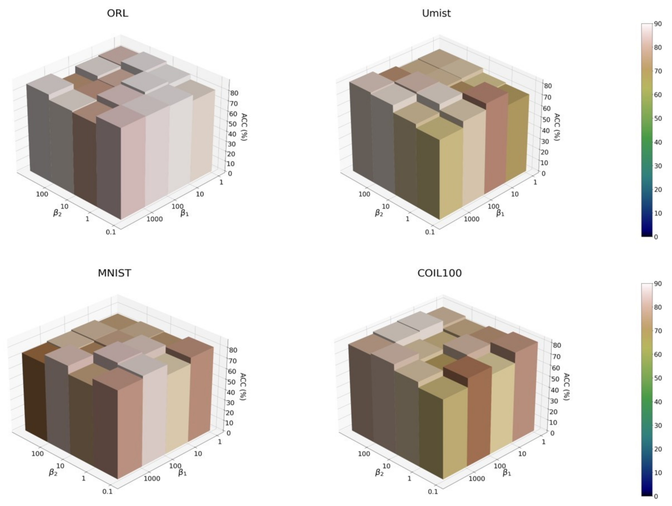
4.4. Hyperparameter Sensitivity Analysis

There are two hyper-parameters ${\beta }_1$ and ${\beta }_2$ in H-DSC. Broadly speaking, they are data-dependent; thus, we conducted the grid search to find the optimal hyperparameter values for each dataset. To demonstrate their influences on clustering performance, we searched the ${\beta }_1$ in [1, 10, 100, 1000] and ${\beta }_2$ in [0.1, 1, 10, 100], and then plotted the corresponding ACC performance on four benchmark datasets in Figure 2. From the figure, one can see that although optimal hyperparameter values for the ACC performance varies in different datasets, H-DSC performed stably in a wide range of values across the four benchmark datasets.

4.5. Convergence Behaviors

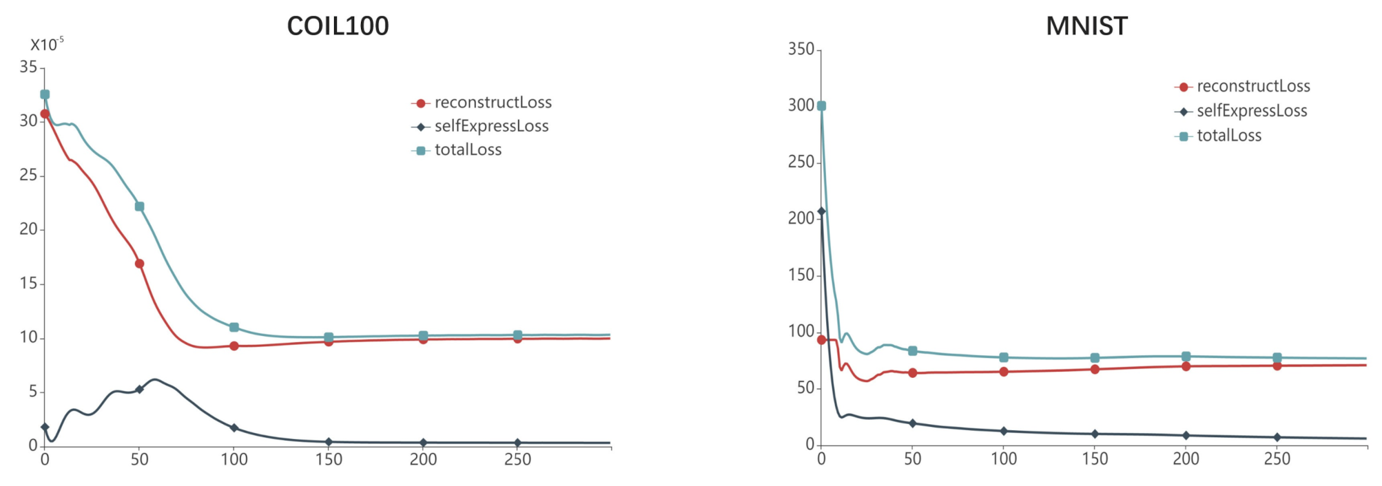
To demonstrate the convergence behavior of H-DSC during training iterations, we conducted experiments on MNIST and COIL100, with ${\beta }_1={\beta }_2=1$. We recorded the hypergraph-supervised reconstruction, self-expression, total cost in Equation (11) during the training process, and plotted them as a function of the number of epochs in Figure 3. As can be seen, the cost functions Equation (11) converge in both datasets when the training epochs are larger than 50.

5. Conclusions

This paper proposes a hypergraph-supervised DSC method to simultaneously enhance the feature learning of deep AE and subspace clustering. In particular, we formulate the hypergraph-supervised reconstruction that guides the decoder of AE to reconstruct samples, according to the high-order relations in the hypergraph. By capturing the high-order relations, the deep AE is allowed to perform a better discriminative feature learning. In addition, we propose hypergraph learning, based on the self-expression in DSC, presenting a joint learning framework to improve the clustering performance further. Experiments on benchmark high-dimensional datasets demonstrate the effectiveness of our proposed method, compared to several recent competitors.

References

- Chen, H.; Xu, K.; Chen, L.; Jiang, Q. Self-Expressive Kernel Subspace Clustering Algorithm for Categorical Data with Embedded Feature Selection. Mathematics 2021, 9, 1680. [Google Scholar] [CrossRef]
- Vandewalle, V. Multi-Partitions Subspace Clustering. Mathematics 2020, 8, 597. [Google Scholar] [CrossRef] [Green Version]
- Elhamifar, E.; Vidal, R. Sparse subspace clustering. In Proceedings of the 2009 IEEE Conference on Computer Vision and Pattern Recognition, Miami, FL, USA, 20–25 June 2009; pp. 2790–2797. [Google Scholar]
- Elhamifar, E.; Vidal, R. Sparse subspace clustering: Algorithm, theory, and applications. IEEE Trans. Pattern Anal. Mach. Intell. 2013, 35, 2765–2781. [Google Scholar] [CrossRef] [PubMed] [Green Version]
- Vidal, R.; Favaro, P. Low rank subspace clustering (LRSC). Pattern Recognit. Lett. 2014, 43, 47–61. [Google Scholar] [CrossRef] [Green Version]
- Ji, P.; Salzmann, M.; Li, H. Efficient dense subspace clustering. In Proceedings of the IEEE Winter Conference on Applications of Computer Vision, Steamboat Springs, CO, USA, 24–26 March 2014; pp. 461–468. [Google Scholar]
- Zheng, R.; Li, M.; Liang, Z.; Wu, F.X.; Pan, Y.; Wang, J. SinNLRR: A robust subspace clustering method for cell type detection by non-negative and low-rank representation. Bioinformatics 2019, 35, 3642–3650. [Google Scholar] [CrossRef]
- Abavisani, M.; Naghizadeh, A.; Metaxas, D.; Patel, V. Deep Subspace Clustering with Data Augmentation. Adv. Neural Inf. Process. Syst. 2020, 33, 10360–10370. [Google Scholar]
- Ji, P.; Zhang, T.; Li, H.; Salzmann, M.; Reid, I. Deep Subspace Clustering Networks. In Advances in Neural Information Processing Systems; MIT Press: Long Beach, CA, USA, 2017; Volume 30. [Google Scholar]
- Peng, X.; Feng, J.; Zhou, J.T.; Lei, Y.; Yan, S. Deep subspace clustering. IEEE Trans. Neural Networks Learn. Syst. 2020, 31, 5509–5521. [Google Scholar] [CrossRef]
- LeCun, Y.; Bengio, Y.; Hinton, G. Deep learning. Nature 2015, 521, 436–444. [Google Scholar] [CrossRef]
- Peng, X.; Xiao, S.; Feng, J.; Yau, W.Y.; Yi, Z. Deep subspace clustering with sparsity prior. IJCAI 2016, 1925–1931. [Google Scholar]
- Zhang, J.; Li, C.G.; You, C.; Qi, X.; Zhang, H.; Guo, J.; Lin, Z. Self-supervised convolutional subspace clustering network. In Proceedings of the IEEE/CVF Conference on Computer Vision and Pattern Recognition, Long Beach, CA, USA, 15–20 June 2019; pp. 5473–5482. [Google Scholar]
- Mrabah, N.; Bouguessa, M.; Ksantini, R. Adversarial deep embedded clustering: On a better trade-off between feature randomness and feature drift. IEEE Trans. Knowl. Data Eng. 2020. [Google Scholar] [CrossRef]
- Mrabah, N.; Khan, N.M.; Ksantini, R.; Lachiri, Z. Deep clustering with a dynamic autoencoder: From reconstruction towards centroids construction. Neural Netw. 2020, 130, 206–228. [Google Scholar] [CrossRef]
- Wang, S.; Ding, Z.; Fu, Y. Feature selection guided auto-encoder. In Proceedings of the AAAI Conference on Artificial Intelligence, San Francisco, CA, USA, 4–9 February 2017; Volume 31. [Google Scholar]
- Lv, J.; Kang, Z.; Lu, X.; Xu, Z. Pseudo-supervised Deep Subspace Clustering. IEEE Trans. Image Process. 2021, 30, 5252–5263. [Google Scholar] [CrossRef]
- Kang, Z.; Lu, X.; Liang, J.; Bai, K.; Xu, Z. Relation-guided representation learning. Neural Netw. 2020, 131, 93–102. [Google Scholar] [CrossRef]
- Agarwal, S.; Lim, J.; Zelnik-Manor, L.; Perona, P.; Kriegman, D.; Belongie, S. Beyond pairwise clustering. In Proceedings of the Conference on Computer Vision and Pattern Recognition(CVPR), San Diego, CA, USA, 20–26 June 2005; Volume 2, pp. 838–845. [Google Scholar]
- Gao, S.; Tsang, I.W.H.; Chia, L.T. Laplacian sparse coding, hypergraph laplacian sparse coding, and applications. IEEE Trans. Pattern Anal. Mach. Intell. 2012, 35, 92–104. [Google Scholar] [CrossRef]
- Ng, A.Y.; Jordan, M.I.; Weiss, Y. On spectral clustering: Analysis and an algorithm. In Advances in Neural Information Processing Systems; MIT Press: Cambridge, MA, USA, 2002; pp. 849–856. [Google Scholar]
- Yin, M.; Guo, Y.; Gao, J.; He, Z.; Xie, S. Kernel sparse subspace clustering on symmetric positive definite manifolds. In Proceedings of the IEEE Conference on Computer Vision and Pattern Recognition, Las Vegas, NV, USA, 27–30 June 2016; pp. 5157–5164. [Google Scholar]
- Peng, X.; Feng, J.; Xiao, S.; Yau, W.Y.; Zhou, J.T.; Yang, S. Structured autoencoders for subspace clustering. IEEE Trans. Image Process. 2018, 27, 5076–5086. [Google Scholar] [CrossRef]
- Zhou, P.; Hou, Y.; Feng, J. Deep adversarial subspace clustering. In Proceedings of the IEEE Conference on Computer Vision and Pattern Recognition, Salt Lake City, UT, USA, 18–23 June 2018; pp. 1596–1604. [Google Scholar]
- Jiang, Y.; Yang, Z.; Xu, Q.; Cao, X.; Huang, Q. When to learn what: Deep cognitive subspace clustering. In Proceedings of the 26th ACM International Conference on Multimedia, Seoul, Korea, 22–26 October 2018; pp. 718–726. [Google Scholar]
- Kheirandishfard, M.; Zohrizadeh, F.; Kamangar, F. Multi-level representation learning for deep subspace clustering. In Proceedings of the IEEE/CVF Winter Conference on Applications of Computer Vision, Snowmass Village, CO, USA, 1–5 March 2020; pp. 2039–2048. [Google Scholar]
- Xu, Y.; Chen, S.; Li, J.; Han, Z.; Yang, J. Autoencoder-based latent block-diagonal representation for subspace clustering. IEEE Trans. Cybern. 2020, 1–11. [Google Scholar] [CrossRef]
- Valanarasu, J.M.J.; Patel, V.M. Overcomplete Deep Subspace Clustering Networks. In Proceedings of the IEEE/CVF Winter Conference on Applications of Computer Vision, Waikoloa, HI, USA, 3–8 January 2021; pp. 746–755. [Google Scholar]
- Peng, Z.; Jia, Y.; Liu, H.; Hou, J.; Zhang, Q. Maximum Entropy Subspace Clustering Network. IEEE Trans. Circuits Syst. Video Technol. 2021. [Google Scholar] [CrossRef]
- Zhou, D.; Huang, J.; Schölkopf, B. Learning with hypergraphs: Clustering, classification, and embedding. In Advances in Neural Information Processing Systems; MIT Press: Cambridge, MA, USA, 2007; pp. 1601–1608. [Google Scholar]
- Xie, Y.; Zhang, W.; Qu, Y.; Dai, L.; Tao, D. Hyper-Laplacian regularized multilinear multiview self-representations for clustering and semisupervised learning. IEEE Trans. Cybern. 2018, 50, 572–586. [Google Scholar] [CrossRef]
- Peng, Y.; Li, W.; Luo, X.; Du, J. Hyperspectral Image Super-Resolution Using Global Gradient Sparse and Nonlocal Low-rank Tensor Decomposition with Hyper-Laplacian Prior. IEEE J. Sel. Top. Appl. Earth Obs. Remote. Sens. 2021, 14, 5453–5469. [Google Scholar] [CrossRef]
- Huang, S.; Elgammal, A.; Yang, D. On the effect of hyperedge weights on hypergraph learning. Image Vis. Comput. 2017, 57, 89–101. [Google Scholar] [CrossRef] [Green Version]
- Liu, Q.; Sun, Y.; Wang, C.; Liu, T.; Tao, D. Elastic net hypergraph learning for image clustering and semi-supervised classification. IEEE Trans. Image Process. 2016, 26, 452–463. [Google Scholar] [CrossRef] [Green Version]
- Kingma, D.P.; Ba, J. Adam: A Method for Stochastic Optimization. In Proceedings of the 3rd International Conference on Learning Representations (ICLR), San Diego, CA, USA, 7–9 May 2015. [Google Scholar]
- Liu, G.; Lin, Z.; Yan, S.; Sun, J.; Yu, Y.; Ma, Y. Robust recovery of subspace structures by low-rank representation. IEEE Trans. Pattern Anal. Mach. Intell. 2012, 35, 171–184. [Google Scholar] [CrossRef] [Green Version]
- Purkait, P.; Chin, T.J.; Sadri, A.; Suter, D. Clustering with hypergraphs: The case for large hyperedges. IEEE Trans. Pattern Anal. Mach. Intell. 2016, 39, 1697–1711. [Google Scholar] [CrossRef]
Figure 1.
The framework of hypergraph-supervised deep subspace clustering (H-DSC), with the encoder of the AE extract deep feature as ; the self-expression performs subspace clustering on to extract the coefficient matrix . The hypergraph is then learned from and guides the deep AE reconstruction with the cost function . In addition, we incorporate for pseudo-label training to improve clustering performance.
Figure 2.
The ACC performance of our proposed H-DSC, with respect to the varying hyperparameter and on four benchmark datasets.
Figure 3.
The cost function value decay of H-DSC during the training process on COIL100 and MNIST. The vertical and horizontal axis represent the cost function values and number of training epochs, respectively. The red, blue, and green lines indicate the cost function value of , , and , respectively.