Fuzzy Automata as Coalgebras

Abstract

The coalgebraic method is of great significance to research in process algebra, modal logic, object-oriented design and component-based software engineering. In recent years, fuzzy control has been widely used in many fields, such as handwriting recognition and the control of robots or air conditioners. It is then an interesting topic to analyze the behavior of fuzzy automata from a coalgebraic point of view. This paper models different types of fuzzy automata as coalgebras with a monad structure capturing fuzzy behavior. Based on the coalgebraic models, we can define a notion of fuzzy language and consider several versions of bisimulation for fuzzy automata. A group of combinators is defined to compose fuzzy automata of two branches: state transition and output function. A case study illustrates the coalgebraic models proposed and their composition.

1. Introduction

Control logic plays an important role in component-based programming in deciding a run-time mechanisms and rules of composition. Precise control needs meticulous implementation so that many applications may be expensive and inefficient. To tackle this problem, there is an increasing interest in using fuzzy logic in many new areas. As a very efficient method for handling imprecise properties, fuzzy logic then provides a systematic approach to incorporating approximate reasoning into such systems so that fuzzy implementations are not only cheaper and faster than precise ones, but also more understandable for users [1,2]. Therefore, some devices that profit from the use of vagueness in their overall operation have emerged and the related theory is described in [3]. For instance, the fuzzy principal component analysis method, based on the variance contribution rate of the principal component combined with the fuzzy theory to obtain a reasonable correction weight, is used to refine quantitative and qualitative index data of innovation service capability [4]. Moreover, this approach makes sense not only at the control level, but also at the test level [5].

Fuzzy control systems incorporate a number of components driven by fuzzy logic [6]. Most of them are rule-based systems that exchange information through interfaces. Technically, the modeling approach of fuzzy control systems contains three aspects: an input stage, a processing stage and an output stage, whose details are as follows.

• The input stage transforms an input into a value. The method is to abstract the relation of an input and its corresponding vague value into a point in a coordinate system, where the horizontal axis stands for the input domain and the vertical axis stands for the vagueness domain.
• The processing stage involves inference rules and generates a result for each input, and then combines the results of the rule. In this stage, logical inference rules are used to describe the connection between cause and effect. The rules are of the form

  $$\mathtt{If}\langle condition\rangle \mathtt{then}\langle conclusion\rangle .$$

  Such rules provide information for the decision of control variables.
• The output stage processes the combined results from the processing stage and converts them to a specific control value. For instance, common techniques for conversion process includes max-min inference, max-membership principle and mean-max membership.

Automata theory has a long history in modeling systems and applications which can be realized as a set of states and transitions between them depending on some inputs. Fuzzy finite-state automata (FFA) incorporate fuzziness into the internal state representation and output of these computational systems [7]. Depending on the non-fuzzy output labels associated with (final) states or transitions, there are different classes of FFA: FFA with final states, FFA without final states, Fuzzy Moore FA and Fuzzy Mealy FA [8]. There are also works considering fuzzy output maps, such as fuzzy Mealy machines and fuzzy Moore machines [9,10]. Fuzzy automata have been studied from different aspects. In order to study behavior control, a novel method to compute the membership values of the next states of a fuzzy automaton with an averaging function between the membership value of the input, and the membership value of the current state is proposed in [11]; the behaviors of lattice-valued nondeterministic fuzzy automata are compared through two language equivalence relations which have different discriminating power in [12]. Categories of deterministic fuzzy automata and fuzzy languages based on a complete residuated lattice with zero divisors are introduced in [13], a common framework for fuzzy type automata is developed in relationships with morphisms of monads in [14], and the concept of fuzzy regular language accepted by fuzzy finite automata is purposed in [15]. Describing systems that behave in the same way in the sense that one system simulates the other and vice versa, several notions of (approximate) bismulation relations are investigated in [16,17,18].

Along the past two decades, coalgebra has emerged as a well established general framework for the study of the behavior of various kinds of automata [19,20,21]. There is in particular a generalized determinization construction from automata to coalgebras, including partial Mealy machines, (structured) Moore automata, Rabin probabilistic automata, and pushdown automata [22]. A survey and hierarchy of probabilistic systems as coalgebras is discussed in [23]. It connects probabilistic verification with coalgebraic modeling and compares expressiveness of system types by natural transformations between functors. Hybrid automata specifying both discrete and continuous behavior can also be modeled as coalgebras [24]. A coalgebraic perspective supporting a generic theory of hybrid automata with a rich palette of definitions and results is studied in [25]. In addition, a coalgebraic semantics framework for quantum systems is developed in [26]. One obvious advantage of the coalgebraic view is that it induces a simple and intuitive notion of bisimulation between coalgebras, a notion originally stemming from the world of labeled transition systems and process algebra [27,28,29]. Witnessed by the notion of coalgebra homomorphism, bisimulation on coalgebras can be defined by commutative diagrams and shown to be formally dual to congruence on algebra [30,31]. Moreover, there is a general framework for the study of components as concrete coalgebras and the development of the corresponding calculi [32].

A recent thesis [33] proposes a coalgebraic approach to fuzzy automata, which obtains the following results: (a) a coalgebraic definition of the fuzzy language recognized by a fuzzy automaton, (b) the definition of a functor describing the determinization process of a fuzzy automata via a generalization of the powerset construction, (c) a coalgebraic definition of bisimulation on fuzzy automata allowing the construction of a quotient fuzzy automaton. However, it only considers the output as the current membership value for the current state. Moreover, a coalgebraic theory of fuzzy transition systems and their concrete fuzzy bisimulation is studied in [34]. The authors resort to relational lifting that is one of the most used methods in bisimulation research, leading to an algorithm for testing bisimulation in [35], and group-by-group fuzzy bisimulation and its corresponding modal logic in [36]. Nevertheless, the output stage is omitted. To consider different types of fuzzy automata, our main contributions are as follows:

• Explore the fuzzy-set monad to serve as the basis to a coalgebraic approach;
• Provide a coalgebraic framework for different types of fuzzy automata, where the notions of fuzzy language and bisimulation can be addressed;
• Define appropriate combinators for composing fuzzy automata from two branches:state transition and output function.

Thus, we not only consider fuzzy language respecting the controlling behavior and bisimulation relations for fuzzy automata, but also study the composition mechanism in our coalgebraic framework.

This paper is structured as follows. Section 2 introduces different types of fuzzy automata. Section 3 recalls the definition of the fuzzy-set monad and studies its properties. Section 4 defines the coalgebraic models for fuzzy automata, the notion of fuzzy language and considers several versions of bisimulation. Section 5 develops a series of combinators for composing fuzzy automata. Section 6 discusses a case study. Section 7 concludes and raises some topics for future work.

2. Fuzzy Automata

In a complex controlled system driven by fuzzy logic, a fuzzy automaton is the basic unit which contains fuzzy processors and input/output interfaces. Considering fuzzy output maps, we focus on three types of fuzzy automata: Fuzzy Moore Automata (FMrA), Fuzzy Mealy Automata (FMlA) and Fuzzy Unified Automata (FUA). FMrA and FMlA are obtained by modifying the definitions of fuzzy Moore machine and fuzzy Mealy machine in [8]. Unlike the definition of fuzzy Mealy machine in [8] requiring two functions, one to describe the next state and the other to describe the output, a fuzzy Mealy machine is equipped with one fuzzy function to characterize completely the next state and the output produced in [9]. For distinction between them, we name the latter one as FUA. For simplicity, initial and final states are ignored for the moment.

Definition 1 (Fuzzy Moore Automata (FMrA)).

A fuzzy Moore automaton is a 5-tuple $p=(X,I,O,\alpha ,e)$ where

• X is a set of states.
• I is a set of input symbols.
• O is a set of output symbols.
• $\alpha :X\times I\to {[0,1]}^X$is a fuzzy transition function.
• $e:X\to {[0,1]}^O$is a fuzzy output function.

Note that each non-fuzzy output map $e^{\prime }:X\to O$ corresponds to a function $e:X\to {[0,1]}^O$ such that $e(x)={\delta }_{e^{\prime }(x)}$, where ${\delta }_k(t)=\delta (t-k)$ and δ is the Dirac function.

Definition 2 (Fuzzy Mealy Automata (FMlA)).

A fuzzy Mealy automaton is a 5-tuple $p=(X,I,O,\alpha ,e)$ where

• $X,I,O,\alpha :X\times I\to {[0,1]}^X$are defined as in FMrA.
• $e:X\times I\to {[0,1]}^O$is a fuzzy input-output function.

Note that each non-fuzzy output map $e^{\prime }:X\times I\to O$ corresponds to a fuzzy input-output function $e:X\times I\to {[0,1]}^O$ where $e(x,i)={\delta }_{e^{\prime }(x,i)}$.

Given an FMrA $(X,I,O,\alpha ,e)$, it is easy to construct an FMlA $(X,I,O,\alpha ,e^{\prime })$ where $e^{\prime }(x,i)=e(x)$ without loss of information, so we regard it as a subcase of FMlA and concentrate on the study of FMlA as coalgebras.

Definition 3 (Fuzzy Unified Automata (FUA)).

A fuzzy unified automaton is a 4-tuple $p=(X,I,O,\beta )$ where

• $X,I,O$are defined as in FMrA.
• $\beta :X\times I\to {[0,1]}^{X\times O}$is a fuzzy input-transition-output function.

In classical methods, two operations $F_1:[0,1]\times [0,1]\to [0,1]$ and $F_2:{[0,1]}^{\ast }\to [0,1]$ should be defined to to define the language accepted by an automaton [7]. Instead, we intend to define the notion of fuzzy language with the aid of the fuzzy-set monad.

3. Fuzzy-Set Monad

3.1. Fuzzy Set

The fuzzy set theory [37] was developed by Lotfi A. Zadeh in 1965. The main purpose of using fuzzy sets is to deal with vague data under some given properties. For example, consider a finite set of real numbers $S\subseteq \mathbb{R}$ and the property “close to 0”. This property seems ambiguous because there is not an explicit criterion to judge whether objects are closed to 0. We want to ask within what distance we can say “one real number is close to 0”. To make it precise, the one should figure out a function which fits the property. For example,

$${\psi }_S(x)=max\{0,1-\frac{1}{m}\left|x\right|\},x\in [-m,m]$$

where $m=ma{x}_{s\in S}\left|s\right|$. This function is called the membership function and indicates that the closer the data $s\in S$ is to 0, the closer the membership value ${\psi }_S(s)$ is to 0. Obviouly, data from which the distance to 0 are equal have the same membership value, i.e., ${\psi }_S(s)={\psi }_S(-s)$. However, the selection of membership function is not unique and usually depends on the goal of application.

Definition 4

(Residuated Lattice [33]). A residuated lattice is an algebra $\mathcal{K}=(K,\wedge ,\vee ,\otimes ,\to ,0,1)$ with four binary and two nullary operations satisfying:

1 

$(K,\wedge ,\vee ,0,1)$is a lattice with the partial order ≤ which is defined by “$x\le y$ if and only if $x\vee y=y$”. The greatest (least) element is 1(0) that for all $x\in K$, $x\le 1$($x\ge 0$);

2 

$(K,\otimes ,1)$is a commutative monoid with the unit element 1;

3 

For $x,y,z\in K$, $x\le y\to z$ if and only if $x\otimes y\le z$.

Especially, if $(K,\wedge ,\vee ,0,1)$ is a complete lattice, then $\mathcal{K}$ is called a complete residuated lattice.

Residuated lattices are the algebraic structure that characterizes fuzzy components.

Example 1.

The Boolean algebra $(\mathbf{2},\wedge ,\vee ,\neg )$ is a residuated lattice $(\mathbf{2},{\wedge }^{\prime },{\vee }^{\prime },{\otimes }^{\prime },{\to }^{\prime },0,1)$. In this expression, $\mathbf{2}=\{0,1\}$ is the set of elements. ${\wedge }^{\prime },{\vee }^{\prime }$ correspond to ∧ and ∨ operations in Boolean algebra, respectively. Multiplication ${\otimes }^{\prime }$ is defined as ∧. The residuate operation ${\to }^{\prime }$ comes as $x{\to }^{\prime }y:=\neg x\vee y$.

Definition 5

(Fuzzy Subset [33]). Given a set X, a fuzzy subset over $\mathcal{K}$ of X is a function $\varphi :X\to K$ that assigns to each object $x\in X$ a membership value. The set of all fuzzy subsets of X is denoted by $Z_{\mathcal{K}}(X)$ and obviously $Z_{\mathcal{K}}(X)=K^X$. In the sequel, we use the shorthand notation $Z(X)$ to represent $Z_{\mathcal{K}}(X)$.

Note that Z can be interpreted as an endofunctor on $\mathsf{Set}$ where

$$\begin{array}{cc}Z(f):\hfill & K^X\to K^Y\hfill \\ & \kappa \mapsto \lambda y.\underset{x\in f^{-1}(y)}{\bigvee }\kappa (x)\hfill \end{array}$$

for any $f:X\to Y$. Note that

$$\underset{x\in X}{\bigvee }\kappa (x)=\vee \{\kappa (x)|x\in X\}.$$

3.2. Properties of Fuzzy-Set Monad

The fuzzy-set monad on $\mathsf{Set}$ is defined in [33]. In this section, we will firstly recall the definition and then prove this monad is strong and commutative. Although every monad in $\mathsf{Set}$ is strong, we include the explicit contribution to build up intuitions.

Definition 6

(The fuzzy-set Monad [33]). Fuzzy-set monad $\mathbb{Z}=(Z,\eta ,\mu )$ over $\mathcal{K}=(K,\wedge ,\vee ,\otimes ,$$\to ,0,1)$ satisfies for a set X

• $\eta :Id\Rightarrow Z$ satisfies that

  $${\eta }_X(x)(y)=\left\{\begin{array}{cc}1\hfill & x=y\hfill \\ 0\hfill & otherwise,\hfill \end{array}\right.x,y\in X,$$
• $\mu :Z^2\Rightarrow Z$ satisfies that

  $${\mu }_X(\Phi )=\bigcup _{\psi \in Z(X)}\Phi (\psi )⊛\psi ,\Phi \in Z^2(X).$$

  where

  $$(\bigcup _{i\in I}{\varphi }_i)(x)=\underset{i\in I}{\bigvee }{\varphi }_i(x)x\in X,{\varphi }_i\in Z(X)$$

  and

  $$(a⊛\varphi )(x)=a\otimes \varphi (x)a\in K,x\in X,\varphi \in Z(X)$$

Definition 7

(Strong monad [21]). A strong monad is a monad $\mathbb{T}=(T,\eta ,\mu )$ equipped with a left tensorial strength ${\sigma }_{X,Y}:T(X)\times Y\to T(X\times Y)$ that commutes with the unit and multiplication of the monad:

Theorem 1.

The triple $\mathbb{Z}=(Z,\eta ,\mu )$ is a strong monad.

Proof. 

Firstly, define a left tensorial strength with components ${\sigma }_{X,Y}:Z(X)\times Y\to$$Z(X\times Y)$ as

$${\sigma }_{X,Y}(\psi ,y)=\lambda x,\lambda y^{\prime }.(\psi (x)\otimes {\eta }_Y(y)(y^{\prime }))$$

that commute appropriately with trivial projection and associativity isomorphisms for $f:X\to Z$ and $g:Y\to W$:

For the unit,

$$\begin{array}{cc}& {\sigma }_{X,Y}·({\eta }_X\times \mathsf{id})(x,y)\hfill \\ =\hfill & \{\mathrm{Definition}\mathrm{of}\times \}\hfill \\ & {\sigma }_{X,Y}({\eta }_X(x),y)\hfill \\ =\hfill & \{\mathrm{Definition}\mathrm{of}\sigma \}\hfill \\ & \otimes ·({\eta }_X(x)\times {\eta }_Y(y))\hfill \\ =\hfill & \{\mathrm{Definition}\mathrm{of}\eta \}\hfill \\ & {\eta }_{X\times Y}(x,y).\hfill \end{array}$$

For the multiplication, we have to show that ${\mu }_{X\times Y}·Z({\sigma }_{X,Y})·{\sigma }_{Z_{\mathcal{K}}(X),Y}={\sigma }_{X,Y}·({\mu }_X\times \mathsf{id})$. For a pair $(\Phi ,y)\in Z^2(X)\times Y$,

$$\begin{array}{ccc}& {\mu }_{X\times Y}·Z({\sigma }_{X,Y})·{\sigma }_{Z(X),Y}(\Phi ,y)\hfill & \\ =\hfill & \{\mathrm{Definition}\mathrm{of}\sigma \}\hfill \\ & {\mu }_{X\times Y}·Z({\sigma }_{X,Y})(\otimes ·(\Phi \times {\eta }_Y(y)))\hfill \\ =\hfill & \{\mathrm{Definition}\mathrm{of}Z,\sigma \}\hfill \\ & {\mu }_{X\times Y}(\bigcup _{(\psi ,y^{\prime })\in Z(X)\times Y}\otimes ·(\Phi \times {\eta }_Y(y))(\psi ,y^{\prime })⊛{\eta }_{Z(X\times Y)}({\sigma }_{X,Y}(\psi ,y^{\prime })))\hfill \\ =\hfill & \{\otimes ·(f\times g)(x,y)=f(x)\otimes g(y)\}\hfill \\ & {\mu }_{X\times Y}(\bigcup _{(\psi ,y^{\prime })\in Z(X)\times Y}(\Phi (\psi )\otimes {\eta }_Y(y)(y^{\prime }))⊛{\eta }_{Z(X\times Y)}({\sigma }_{X,Y}(\psi ,y^{\prime })))\hfill \\ =\hfill & \{\mathrm{Definition}\mathrm{of}\eta \}\hfill \\ & {\mu }_{X\times Y}(\bigcup _{\psi \in Z(X)}\Phi (\psi )⊛{\eta }_{Z(X\times Y)}({\sigma }_{X,Y}(\psi ,y)))\hfill \\ =\hfill & \{\mathrm{Definition}\mathrm{of}\sigma \}\hfill \\ & {\mu }_{X\times Y}(\bigcup _{\psi \in Z(X)}\Phi (\psi )⊛{\eta }_{Z(X\times Y)}(\otimes ·(\psi \times {\eta }_Y(y))))\hfill \\ =\hfill & \{\mathrm{Definition}\mathrm{of}\mu \}\hfill \\ & \bigcup _{{\psi }^{\prime }\in Z(X\times Y)}(\bigcup _{\psi \in Z(X)}\Phi (\psi )⊛{\eta }_{Z(X\times Y)}(\otimes ·(\psi \times {\eta }_Y(y)))({\psi }^{\prime }))⊛{\psi }^{\prime }\hfill \\ =\hfill & \{\mathrm{Definition}\mathrm{of}\eta \}\hfill \\ & \bigcup _{\psi \in Z(X)}\Phi (\psi )⊛(\otimes ·(\psi \times {\eta }_Y(y))\hfill \end{array}$$

For the right side of the equation,

$$\begin{array}{ccc}& {\sigma }_{X,Y}·({\mu }_X\times \mathsf{id})(\Phi ,y)\hfill & \\ =\hfill & \{\mathrm{Definition}\mathrm{of}\mu \}\hfill \\ & {\sigma }_{X,Y}(\bigcup _{\psi \in Z(X)}\Phi (\psi )⊛\psi ,y)\hfill \\ =\hfill & \{\mathrm{Definition}\mathrm{of}\sigma \}\hfill \\ & \otimes ·((\bigcup _{\psi \in Z(X)}\Phi (\psi )⊛\psi )\times {\eta }_Y(y))\hfill \\ =\hfill & \{\mathrm{Distributive}\mathrm{law}:\otimes ·({\cup }_i{f}_i\times g)={\cup }_i(\otimes ·(f_i\times g))\}\hfill \\ & \bigcup _{\psi \in Z(X)}\otimes ·(\Phi (\psi )⊛\psi \times {\eta }_Y(y))\hfill \\ =\hfill & \{\mathrm{Constant}\Phi (\psi )\}\hfill \\ & \bigcup _{\psi \in Z(X)}\Phi (\psi )⊛(\otimes ·(\psi \times {\eta }_Y(y)).\hfill \end{array}$$

□

In the proof of Theorem 1, we defined a left tensorial strength $\sigma$ with components ${\sigma }_{X,Y}:Z(X)\times Y\to Z(X\times Y)$ as

$${\sigma }_{X,Y}(\psi ,y)=\otimes ·(\psi ,{\eta }_Y(y))=\lambda x,\lambda y^{\prime }.(\psi (x)\otimes {\eta }_Y(y)(y^{\prime })).$$

Of course, a “swapped” tensorial strength ${\sigma }^{\prime }$ with components ${\sigma }_{X,Y}^{\prime }:X\times Z(Y)\to Z(X\times Y)$ can be obtained by applying swapping operation from the left tensorial strength:

$$(X\times Z(Y)\underset{\cong }{\overset{\mathsf{s}}{\to }}Z(Y)\times X\stackrel{{\sigma }_{Y,X}}{\to }Z(Y\times X)\underset{\cong }{\overset{Z(\mathsf{s})}{\to }}Z(X\times Y)).$$

where $\mathsf{s}\widehat{=}\langle {\pi }_2,{\pi }_1\rangle$ is product communicating. Formally,

$${\sigma }_{X,Y}^{\prime }=\otimes ·({\eta }_X(x)\times \varphi )=\lambda x^{\prime }.\lambda y.({\eta }_X(x)(x^{\prime })\otimes \varphi (y)).$$

With both ${\sigma }_{X,Y}$ and ${\sigma }_{X,Y}^{\prime }$, there are two ways to obtain $Z(X)\times Z(Y)\to Z(X\times Y)$, as depicted in the following diagram. If the diagram commutes, then Z is commutative with left and right strength natural transformations ${\sigma }_{X,Y},{\sigma }_{X,Y}^{\prime }$. We use $\gamma :Z(X)\times Z(Y)\to Z(X\times Y)$ to denote the composed arrow.

Theorem 2.

The triple $(Z,\eta ,\mu )$ is a commutative monad.

Proof. 

To show the diagram is commutative, select a pair of membership functions $({\psi }_1,{\psi }_2)\in Z(X)\times Z(Y)$, then

$$\begin{array}{ccc}& {\mu }_{X\times Y}·Z({\sigma }_{X,Y}^{\prime })·{\sigma }_{X,Z(Y)}({\psi }_1,{\psi }_2)\hfill & \\ =\hfill & \{\mathrm{Definition}\mathrm{of}\sigma \}\hfill \\ & {\mu }_{X\times Y}(Z({\sigma }_{X,Y}^{\prime })(\otimes ·({\psi }_1\times {\eta }_{Z(Y)}({\psi }_2)))\hfill \\ =\hfill & \{\mathrm{Definition}\mathrm{of}Z\}\hfill \\ & {\mu }_{X\times Y}(\bigcup _{(x,\psi )\in X\times Z(Y)}\otimes ·({\psi }_1\times {\eta }_{Z(Y)}({\psi }_2))(x,\psi )⊛{\eta }_{Z(X\times Y)}({\sigma }_{X,Y}^{\prime }(x,\psi )))\hfill \\ =\hfill & \{\otimes ·(f\times g)(x,y)=f(x)\otimes g(y)\}\hfill \\ & {\mu }_{X\times Y}(\bigcup _{(x,\psi )\in X\times Z(Y)}({\psi }_1(x)\otimes {\eta }_{Z(Y)}({\psi }_2)(\psi ))⊛{\eta }_{Z(X\times Y)}({\sigma }_{X,Y}^{\prime }(x,\psi )))\hfill \\ =\hfill & \{\mathrm{Definition}\mathrm{of}\eta \}\hfill \\ & {\mu }_{X\times Y}(\bigcup _{x\in X}{\psi }_1(x)⊛{\eta }_{Z(X\times Y)}({\sigma }_{X,Y}^{\prime }(x,{\psi }_2)))\hfill \\ =\hfill & \{\mathrm{Definition}\mathrm{of}{\sigma }^{\prime }\}\hfill \\ & {\mu }_{X\times Y}(\bigcup _{x\in X}{\psi }_1(x)⊛{\eta }_{Z(X\times Y)}(\otimes ·({\eta }_X(x)\times {\psi }_2)))\hfill \\ =\hfill & \{\mathrm{Definition}\mathrm{of}\mu \}\hfill \\ & \bigcup _{{\psi }^{\prime }\in Z(X\times Y)}(\bigcup _{x\in X}{\psi }_1(x)⊛{\eta }_{Z(X\times Y)}(\otimes ·({\eta }_X(x)\times {\psi }_2))({\psi }^{\prime })⊛{\psi }^{\prime })\hfill \\ =\hfill & \{\mathrm{Definition}\mathrm{of}\eta \}\hfill \\ & \bigcup _{x\in X}({\psi }_1(x)⊛(\otimes ·({\eta }_X(x)\times {\psi }_2)))\hfill \\ \widehat{=}\hfill & \{\mathrm{Denotation}\}\hfill \\ & f_1\hfill \end{array}$$

For the right side of the equation,

$$\begin{array}{ccc}& {\mu }_{X\times Y}·Z({\sigma }_{X,Y})·{\sigma }_{Z(X),Y}^{\prime }({\psi }_1,{\psi }_2)\hfill & \\ =\hfill & \{\mathrm{Definition}\mathrm{of}\sigma \}\hfill \\ & {\mu }_{X\times Y}(Z({\sigma }_{X,Y})(\otimes ·({\eta }_{Z(X)}({\psi }_1)\times {\psi }_2)))\hfill \\ =\hfill & \{\mathrm{Definition}\mathrm{of}Z\}\hfill \\ & {\mu }_{X\times Y}(\bigcup _{(\psi ,y)\in Z(X)\times Y}\otimes ·({\eta }_{Z(X)}({\psi }_1)\times {\psi }_2)(\psi ,y)⊛{\eta }_{Z(X\times Y)}({\sigma }_{X,Y}(\psi ,y)))\hfill \\ =\hfill & \{\otimes ·(f\times g)(x,y)=f(x)\otimes g(y)\}\hfill \\ & {\mu }_{X\times Y}(\bigcup _{(\psi ,y)\in Z(X)\times Y}({\eta }_{Z(X)}({\psi }_1)(\psi )\otimes {\psi }_2(y))⊛{\eta }_{Z(X\times Y)}({\sigma }_{X,Y}(\psi ,y)))\hfill \\ =\hfill & \{\mathrm{Definition}\mathrm{of}\eta \}\hfill \\ & {\mu }_{X\times Y}(\bigcup _{y\in Y}{\psi }_2(y)\otimes {\eta }_{Z(X\times Y)}({\sigma }_{X,Y}({\psi }_1,y)))\hfill \\ =\hfill & \{\mathrm{Definition}\mathrm{of}\sigma \}\hfill \end{array}$$

$$\begin{array}{cc}& {\mu }_{X\times Y}(\bigcup _{y\in Y}{\psi }_2(y)⊛{\eta }_{Z(X\times Y)}(\otimes ·({\psi }_1\times {\eta }_Y(y))))\hfill \\ =\hfill & \{\mathrm{Definition}\mathrm{of}\mu \}\hfill \\ & \bigcup _{{\psi }^{\prime }\in Z(X\times Y)}(\bigcup _{y\in Y}{\psi }_2(y)⊛{\eta }_{Z(X\times Y)}(\otimes ·({\psi }_1\times {\eta }_Y(y)))({\psi }^{\prime })⊛{\psi }^{\prime })\hfill \\ =\hfill & \{\mathrm{Definition}\mathrm{of}\eta \}\hfill \\ & \bigcup _{y\in Y}({\psi }_2(y)⊛(\otimes ·({\psi }_1\times {\eta }_Y(y))))\hfill \\ \widehat{=}\hfill & \{\mathrm{Denotation}\}\hfill \\ & f_2\hfill \end{array}$$

Note that $f_1(x,y)={\psi }_1(x)\otimes {\psi }_2(y)=\otimes ·({\psi }_1\times {\psi }_2)(x,y)=f_2(x,y)$. Hence the diagram commutes. □

4. Going Coalgebraic

4.1. Coalgebraic Models

Since the automata introduced in Section 2 are defined over the interval $[0,1]$, we assume the fuzzy-set monad $\mathbb{Z}=(Z,\eta ,\mu )$ is also defined over some complete residuated lattice $([0,1],min,max,\otimes ,\to ,0,1)$. The corresponding coalgebraic models are based on the fuzzy-set monad.

Example 2

([33]). Note that $([0,1],min,max,0,1)$ is a complete lattice. Then there are several ways to construct complete residuated lattices $([0,1],min,max,\otimes ,\to ,0,1)$; namely

• Define

  $$\begin{array}{cc}x\otimes y\hfill & =max(x+y-1,0)\hfill \\ x\to y\hfill & =min(1-x+y,1)\hfill \end{array}$$

  for $x,y\in [0,1]$. Then, $([0,1],min,max,\otimes ,\to ,0,1)$ is a complete residuated lattice corresponding to the standard Lukasiewicz algebra.
• Define

  $$\begin{array}{cc}x\otimes y\hfill & =min(x+y-1,0)\hfill \\ x\to y\hfill & \left\{\begin{array}{cc}1& \mathit{if}x\le y\\ y& \mathit{if}y<x\end{array}\right.\hfill \end{array}$$

  for $x,y\in [0,1]$. Then, $([0,1],min,max,\otimes ,\to ,0,1)$ is a complete residuated lattice corresponding to the standard Gödel algebra.
• Define

  $$\begin{array}{cc}x\otimes y\hfill & =x·y\hfill \\ x\to y\hfill & \left\{\begin{array}{cc}1& \mathit{if}x\le y\\ \frac{y}{x}& \mathit{if}y<x\end{array}\right.\hfill \end{array}$$

  for $x,y\in [0,1]$. Then, $([0,1],min,max,\otimes ,\to ,0,1)$ is a complete residuated lattice corresponding to the standard product algebra.

Consider the two functors $F_{I,O}=Z{(-\times O)}^I$ and $T_{l,O}=Z{(-)}^I\times Z{(O)}^I$. Given a FMlA $(X,I,O,\alpha ,e)$, the corresponding $T_{I,O}$-coalgebra is $(X,\langle \overline{\alpha },\overline{e}\rangle :X\to Z{(X)}^I\times Z{(O)}^I)$ where $\overline{f}$ is the curried version of f. Given a FUA $(X,I,O,\beta )$, the corresponding $F_{I,O}$-coalgebra is $(X,\overline{\beta }:X\to Z{(X\times O)}^I)$. Obviously, there is a natural transformation $\theta$ from $T_{I,O}$ to $F_{I,O}$:

$$\theta (\langle f,g\rangle )(i)=\gamma (\langle f(i),g(i)\rangle )$$

for $f\in Z{(X)}^I,g\in Z{(O)}^I$ and $i\in I$. In the sequel, $F_{I,O}$-coalgebras provide a universal framework for defining fuzzy language and bisimulation for different fuzzy automata while $T_{I,O}$-coalgebras serve as a basis for composition calculi of fuzzy Mealy automata.

4.2. Fuzzy Language

In [33], fuzzy automata with initial fuzzy subsets and final fuzzy subsets are equipped with the notion of fuzzy language over a set of input symbols. Due to the type of their initial/final fuzzy subsets, that notion can not be naturally extended to the case involving output. Here we consider the notion of fuzzy language over a set of input symbols and a set of output symbols based on $F_{I,O}$-coalgebras.

Definition 8.

Let $(X,f)$ be an $F_{I,O}$-coalgebra. Define $f^{\ast }:X\to Z{(X\times O^{\ast })}^{I^{\ast }}$ as follows:

$$\begin{array}{cc}\hfill f^{\ast }(x)(i)(y,o)& =f(x)(i)(y,o)\hfill \\ \hfill f^{\ast }(x)(\varnothing )(y,\varnothing )& =\left\{\begin{array}{cc}1& \mathit{if}x=y\\ 0& \mathit{if}x\ne y\end{array}\right.\hfill \\ \hfill f^{\ast }(x)(i)(y,\varnothing )& =0\hfill \\ \hfill f^{\ast }(x)(\varnothing )(y,o)& =0\hfill \\ \hfill f^{\ast }(x)(wi)(y,vo)& =\underset{z\in X}{\bigvee }{f}^{\ast }(x)(w)(z,v)\otimes f^{\ast }(z)(i)(y,o)\hfill \end{array}$$

for $\forall x,y\in X,i\in I,o\in O,w\in I^{\ast },v\in O^{\ast }$. Note that ∅ represents the empty input/output.

Lemma 1.

Given an $F_{I,O}$-coalgebra $(X,f)$, $\forall x,y\in X,w\in I^{\ast },v\in O^{\ast }$, if $\left|w\right|\ne \left|v\right|$ then

$$f^{\ast }(x)(w)(y,v)=0.$$

Proof. 

First, we prove the result for $\left|w\right|>\left|v\right|$ by induction on $\left|w\right|=n$. Let $x,y\in X,w\in I^{\ast },v\in O^{\ast }$. If $n=0$, there exists no v such that $\left|v\right|<0$ and hence the result holds. If $n=1$, then $v=\varnothing$ and the result holds by the Definition 8. Assume that the result is true for all $\left|w\right|\in I^{\ast }$ such that $\left|w\right|=n-1,n>1$. Now there are two cases: $\left|v\right|=\varnothing$ and $\left|v\right|\ne \varnothing$. For the case $\left|v\right|=\varnothing$, let $\left|w\right|=w^{\prime }i$, where $\left|w\right|=n,i\in I$, and then

$$f^{\ast }(x)(w^{\prime }i)(y,\varnothing )=\underset{z\in X}{\bigvee }{f}^{\ast }(x)(w^{\prime })(z,\varnothing )\otimes f^{\ast }(z)(i)(y,\varnothing ).$$

By the induction hypothesis, $f^{\ast }(x)(w^{\prime })(z,\varnothing )=f^{\ast }(z)(i)(y,\varnothing )=0$ and thus the result holds. For the case $\left|v\right|\ne \varnothing$, let $w=w^{\prime }i,v=v^{\prime }o$ where $\left|w\right|=n>\left|y\right|,i\in I,o\in O$ and then

$$f^{\ast }(x)(w^{\prime }i)(y,v^{\prime }o)=\underset{z\in X}{\bigvee }{f}^{\ast }(x)(w^{\prime })(z,v^{\prime })\otimes f^{\ast }(z)(i)(y,o).$$

By the induction hypothesis, $f^{\ast }(x)(w^{\prime })(z,v^{\prime })=0$ and hence $\forall z\in X,f^{\ast }(x)(w^{\prime })(z,v^{\prime })\otimes f^{\ast }(z)(i)(y,o)=0$. Therefore, the result holds.

Second, by a similar proof, we can prove the result holds for $\left|w\right|<\left|v\right|$ by induction on $\left|y\right|=n$. □

Lemma 2.

Given an $F_{I,O}$-coalgebra $(X,f)$, $\forall x,y\in X$, $w_1,w_2\in I^{\ast }$, $v_1,v_2\in O^{\ast }$, if $|w_1|=|v_1|$ and $|w_2|=|v_2|$, then

$$f^{\ast }(x)(w_1{w}_2)(y,v_1{v}_2)=\underset{z\in X}{\bigvee }{f}^{\ast }(x)(w_1)(z,v_1)\otimes f^{\ast }(z)(w_2)(y,v_2)$$

Proof. 

The results can be proved by induction on $|w_2|=n$. If $n=0$, then $w_2=v_2=\varnothing$ and $w_1{w}_2=w_1,v_1{v}_2=v_1$. Since $f^{\ast }(x)(\varnothing )(y,\varnothing )$ is 1 when $x=y$ and $f^{\ast }(x)(\varnothing )(y,\varnothing )$ is 0 otherwise,

$$f^{\ast }(x)(w_1)(y,v_1)=\underset{z\in X}{\bigvee }{f}^{\ast }(x)(w_1)(z,v_1)\otimes f^{\ast }(z)(\varnothing )(y,\varnothing )$$

holds, which completes the proof of the base case. Now assume that the result is true for all $|w_2|=n-1,n>0$. Let $w_2=w^{\prime }i$ and $v_2=v^{\prime }o$, where $|w^{\prime }|=|v^{\prime }|=n-1,i\in I,$$o\in O$. Then

$$\begin{array}{cc}& f^{\ast }(x)(w_1{w}_2)(y,v_1{v}_2)\hfill \\ =\hfill & f^{\ast }(x)(w_1{w}^{\prime }i)(y,v_1{v}^{\prime }o)\hfill \\ =\hfill & \underset{z\in X}{\bigvee }{f}^{\ast }(x)(w_1{w}^{\prime })(z,v_1{v}^{\prime })\otimes f^{\ast }(z)(i)(y,o)\hfill \\ =\hfill & \underset{z\in X}{\bigvee }(\underset{r\in X}{\bigvee }{f}^{\ast }(x)(w_1)(r,v_1)\otimes f^{\ast }(r)(w^{\prime })(y,v^{\prime }))\otimes f^{\ast }(z)(i)(y,o)\hfill \\ =\hfill & \underset{z\in X}{\bigvee }(\underset{r\in X}{\bigvee }{f}^{\ast }(x)(w_1)(r,v_1)\otimes f^{\ast }(r)(w^{\prime })(y,v^{\prime })\otimes f^{\ast }(z)(i)(y,o))\hfill \\ =\hfill & \underset{r\in X}{\bigvee }(\underset{z\in X}{\bigvee }{f}^{\ast }(x)(w_1)(r,v_1)\otimes f^{\ast }(r)(w^{\prime })(y,v^{\prime })\otimes f^{\ast }(z)(i)(y,o))\hfill \\ =\hfill & \underset{r\in X}{\bigvee }(f^{\ast }(x)(w_1)(r,v_1)\otimes \underset{z\in X}{\bigvee }{f}^{\ast }(r)(w^{\prime })(y,v^{\prime })\otimes f^{\ast }(z)(i)(y,o))\hfill \\ =\hfill & \underset{r\in X}{\bigvee }{f}^{\ast }(x)(w_1)(r,v_1)\otimes f^{\ast }(r)(w^{\prime }i)(y,v^{\prime }o)\hfill \\ =\hfill & \underset{r\in X}{\bigvee }{f}^{\ast }(x)(w_1)(r,v_1)\otimes f^{\ast }(r)(w_2)(y,v_2)\hfill \end{array}$$

□

Now we consider a generic fuzzy language for $F_{I,O}$-coalgebras and naturally obtain the definition for the fuzzy language accepted by a fuzzy automaton.

Definition 9 (Fuzzy language).

A fuzzy language over an input set I and an output set O (with membership values over $\mathcal{K}$), is a fuzzy subset of ${(IO)}^{\ast }$, that is a function $\varphi :{(IO)}^{\ast }\to [0,1]$.

Example 3.

For instance, let $I=\{i_1,i_2\},O=\{o_1,o_2\}$. A fuzzy language ϕ can be defined as $\varphi (i_1{o}_1)=0.6,\varphi (i_1{o}_2)=0.8,\varphi (i_2{o}_1)=0.5,\varphi (i_2{o}_2)=1$ and $\varphi (s)=0,\forall s\in {(IO)}^{\ast },\left|s\right|\ne 2$.

Definition 10.

Consider an $F_{I,O}$-coalgebra $(X,f:X\to Z{(X\times O)}^I)$. For $w=i_1{o}_1{i}_2{o}_2\cdots \in {(IO)}^{\ast }$, define $w_i=i_1{i}_2\cdots$ and $w_o=o_1{o}_2\cdots$. Given an initial fuzzy state $ϵ\in Z(X)$ and a final fuzzy state $\tau \in Z(X)$, the fuzzy language $L_f$ recognized by $(X,f)$ is defined by

$$L_f(w)=\underset{x,y\in X}{\bigvee }ϵ(x)\otimes f^{\ast }(x)(w_i)(y,w_o)\otimes \tau (y),w\in {(IO)}^{\ast }.$$

Naturally, the fuzzy language recognized by a FUA $(X,I,O,\beta )$ is the one recognized by its corresponding $F_{I,O}$-coalgebra $(X,\overline{\beta })$.

When considering the language recognized by an FMlA, the membership values of the next state and the output must be integrated, which can be captured by the natural transformation $\theta$.

Definition 11.

The fuzzy language recognized by a FMlA $(X,I,O,\alpha ,e)$ is the one recognized by the corresponding $F_{I,O}$-coalgebra $(X,\theta (\langle \overline{\alpha },\overline{e}\rangle ))$.

4.3. Bisimulation

Let us now discuss the notion of bisimulation for fuzzy automata. In fact, coalgebra theory provides a generic notion of bisimulation on H-coalgebras for any functor H [20].

Definition 12 (H-bisimulation).

Given two H-coalgebras $(X,f:X\to H(X))$ and $(Y,g:Y\to H(Y))$, an H-bisimulation between them is a relation $R\subseteq X\times Y$ such that there exists an H-coalgebra $(R,h:R\to H(R))$ making the following diagram to commute.

Theorem 3.

Given two $T_{I,O}$-coalgebras $(X,f)$ and $(Y,g)$, if $R\subseteq X\times Y$ is a $T_{I,O}$-bisimulation, then R is an $F_{I,O}$-bisimulation between $(X,\theta \circ f)$ and $(X,\theta \circ g)$.

Proof. 

The proof of the result is immediate from the definition. □

We now consider concrete bisimulations for different types of fuzzy automata. Since FMrA can be easily transformed to FMlA, we only focus on bisimulation for FMlA and FUA. Given a FMlA $(X,I,O,\alpha ,e)$, denote a transition $x\underset{o,v_2}{\overset{i,v_1}{\to }}{x}^{\prime }$ if $\alpha (x,i)(x^{\prime })=v_1,e(x,i)(o)=v_2$. Given a FUA $(X,I,O,\beta )$, denote a transition $x\stackrel{i\left|v\right|o}{\to }{x}^{\prime }$ if $\beta (x,i)(x^{\prime },o)=v$.

Definition 13 (Bisimulation for FMlA).

Given two FMlA $(X,I,O,\alpha ,e)$ and $(Y,I,O,{\alpha }^{\prime },e^{\prime })$, $R\subseteq X\times Y$ is a concrete bisimulation if it satisfies the following properties.

• For $(x,y)\in R$, if $x\underset{o,v_2}{\overset{i,v_1}{\to }}{x}^{\prime }$, there exists $y^{\prime }\in Y$, such that $y\underset{o,v_2}{\overset{i,v_1}{\to }}{y}^{\prime }$ and $(x^{\prime },y^{\prime })\in R$.
• For $(x,y)\in R$, if $y\underset{o,v_2}{\overset{i,v_1}{\to }}{y}^{\prime }$, there exists $x^{\prime }\in X$, such that $x\underset{o,v_2}{\overset{i,v_1}{\to }}{x}^{\prime }$ and $(x^{\prime },y^{\prime })\in R$.

Definition 14 (Bisimulation for FUA).

Given two FUA $p=(X,I,O,\beta )$ and $q=(Y,I,O,{\beta }^{\prime })$, $R\subseteq X\times Y$ is a concrete bisimulation if it satisfies the following properties.

• For $(x,y)\in R$, if $x\stackrel{i\left|v\right|o}{\to }{x}^{\prime }$, there exists $y^{\prime }\in Y$, such that $y\stackrel{i\left|v\right|o}{\to }{y}^{\prime }$ and $(x^{\prime },y^{\prime })\in R$.
• For $(x,y)\in R$, if $y\stackrel{i\left|v\right|o}{\to }{y}^{\prime }$, there exists $x^{\prime }\in X$, such that $x\stackrel{i\left|v\right|o}{\to }{x}^{\prime }$ and $(x^{\prime },y^{\prime })\in R$.

Theorem 4.

Given two FMlA $(X,I,O,\alpha ,e)$ and $(Y,I,O,{\alpha }^{\prime },e^{\prime })$, R is a concrete bisimulation if and only if R is a $T_{I,O}$-bisimulation between their corresponding $T_{I,O}$-coalgebras.

Proof. 

The proof of the result is immediate from the definition. □

Theorem 5.

Given two FUA $(X,I,O,\beta )$ and $(Y,I,O,{\beta }^{\prime })$, R is a concrete bisimulation if and only if R is an $F_{I,O}$-bisimulation between their corresponding $F_{I,O}$-coalgebras.

Proof. 

The proof of the result is immediate from the definition. □

Since the core idea of fuzzy automata is fuzzing, the concrete bisimulation induced by coalgebraic bisimulation seems to be too strict. To find a more suitable characterization of bisimulation of fuzzy automata, we introduce the notion of approximate $ϵ$-bisimulation, which requires that membership values for states in an approximate $ϵ$-bisimulation of two transition branches should have a difference less than $ϵ$.

Definition 15 ($ϵ$-Bisimulation for FMlA).

Given two FMlA $(X,I,O,\alpha ,e)$ and $(Y,I,O,{\alpha }^{\prime },e^{\prime })$, a relation $R\subseteq X\times Y$ is an approximate ϵ-bisimulation ($ϵ>0$) if for all $(x,y)\in R$:

• If $x\underset{o,v_2}{\overset{i,v_1}{\to }}{x}^{\prime }$, there exists $y^{\prime }\in Y$, such that $y\underset{o,u_2}{\overset{i,u_1}{\to }}{y}^{\prime },|u_1-v_1|\le ϵ,|u_2-v_2|\le ϵ$ and $(x^{\prime },y^{\prime })\in R$.
• If $y\underset{o,u_2}{\overset{i,u_1}{\to }}{y}^{\prime }$, there exists $x^{\prime }\in X$, such that $x\underset{o,v_2}{\overset{i,v_1}{\to }}{x}^{\prime },|u_1-v_1|\le ϵ,|u_2-v_2|\le ϵ$ and $(x^{\prime },y^{\prime })\in R$.

Example 4.

Consider two FMlA $(X,I,O,\alpha ,e)$ and $(Y,I,O,{\alpha }^{\prime },e^{\prime })$, where $X=\{x_1,x_2\},Y=\{y_1,y_2\},I=\{i\},O=\{o\},\alpha (x_1,i)(x_2)=0.6,e(x_1,i)(o)=0.4,{\alpha }^{\prime }(y_1,i)(y_2)=0.5,e^{\prime }(y_1,i)(o)$ = 0.5. Then, $R=\{(x_1,y_1),(x_2,y_2)\}$ is an approximate $0.1$-bisimulation.

Definition 16 ($ϵ$-Bisimulation for FUA).

Given two FUA $(X,I,O,\beta )$ and $(Y,I,O,{\beta }^{\prime })$, a relation $R\subseteq X\times Y$ is an approximate ϵ-bisimulation ($ϵ>0$) if for all $(x,y)\in R$,

• If $x\stackrel{i\left|u\right|o}{\to }{x}^{\prime }$, then there exists $y^{\prime }$ such that $y\stackrel{i\left|v\right|o}{\to }{y}^{\prime }$, $|u-v|\le ϵ$ and $(x^{\prime },y^{\prime })\in R;$
• If $y\stackrel{i\left|v\right|o}{\to }{y}^{\prime }$, then there exists $x^{\prime }$ such that $x\stackrel{i\left|u\right|o}{\to }{x}^{\prime }$, $|u-v|\le ϵ$ and $(x^{\prime },y^{\prime })\in R.$

Example 5.

Consider two FUA $(X,I,O,\beta )$ and $(Y,I,O,{\beta }^{\prime })$, where $X=\{x_1,x_2\},Y=\{y_1,y_2\},$ I = $\{i\},O=\{o\},\beta (x_1,i)(x_2,o)=0.8,{\beta }^{\prime }(y_1,i)(y_2,o)=0.7$. Then, $R=\{(x_1,y_1),(x_2,y_2)\}$ is an approximate $0.1$-bisimulation.

Proposition 1.

For approximate ϵ-bisimulation, we have

1.

R is an approximate ϵ-bisimulation if and only if $R^{-1}$ is an approximate ϵ-bisimulation.

2.

If $R_i$ is an approximate ${ϵ}_i$-bisimulation for $i=1,2$, then $R_1\circ R_2$ is an approximate $({ϵ}_1+{ϵ}_2)$ -bisimulation.

3.

If $R_i$ is an approximate ${ϵ}_i$-bisimulation, then ${\cup }_i{R}_i$ is an approximate $ma{x}_i\{{ϵ}_i\}$-bisimulation.

Proof. 

The proof of the result is immediate from the definition. □

5. Composition for FMlA

A family of combinators for $B{(-\times O)}^I$-coalgebras where B is a monad, such as sequential composition $(;)$, parallel $(⊠)$, choice $(⊞)$ and concurrency $(⊡)$ combinators were introduced in [32]. Therefore, the composition of FUA can be naturally instantiated. However, an FMlA assigns different membership values to the next state and the corresponding output, which should be separated for composition. With some abuse of notation, we construct sequential composition $(;)$, parallel $(⊠)$, choice $(⊞)$ and concurrency $(⊡)$ combinators for FMlA. Consider three fuzzy Mealy automata $p,q,r$ with the corresponding coalgebras

$$\begin{array}{cc}〚p〛\hfill & =(X_p,\langle \overline{{\alpha }_p},\overline{e_p}\rangle :X_p\to Z{(X_p)}^I\times Z{(O)}^I)\hfill \\ 〚q〛\hfill & =(X_q,\langle \overline{{\alpha }_q},\overline{e_q}\rangle :X_q\to Z{(X_q)}^J\times Z{(R)}^J)\hfill \\ 〚r〛\hfill & =(X_r,\langle \overline{{\alpha }_r},\overline{e_r}\rangle :X_r\to Z{(X_r)}^O\times Z{(R)}^O).\hfill \end{array}(\star )$$

Some standard isomorphisms in $\mathsf{Set}$ are used in the definitions of combinators:

$$\begin{array}{cc}\hfill \mathsf{a}:& A\times B\times C\to A\times (B\times C)\hfill \\ \hfill \mathsf{s}:& A\times B\to B\times A\hfill \\ \hfill \mathsf{xr}:& A\times B\times C\to A\times C\times B\hfill \\ \hfill \mathsf{m}:& A\times B\times (C\times D)\to A\times C\times (B\times D)\hfill \\ \hfill \mathsf{dist}:& A\times (B+C)\to A\times B+A\times C\hfill \end{array}$$

Furthermore, combinators ${\mathtt{a}}_{+},{\mathtt{s}}_{+},{\mathtt{xr}}_{+},{\mathtt{m}}_{+}$ are the corresponding isomorphisms for sums in $\mathsf{Set}$. Finally, the inverse of an isomorphism i is denoted by $i^{-1}$.

The sequential composition combinator; requires the compatibility of interfaces. The sequential composition of $p,r$ actually shares the data which is sent out from p. From a coalgebraic point of view, it is a $T_{I,R}$-coalgebra

$$〚p;r〛=(X_p\times X_r,\langle \overline{{\alpha }_{p;r}},\overline{e_{p;r}}\rangle )$$

where ${\alpha }_{p;r}$ is defined as:

$$\begin{array}{cc}{X}_p\times X_r\times I\hfill & \stackrel{\mathtt{xr}}{\to }{X}_p\times I\times X_r\stackrel{\langle {\alpha }_p,e_p\rangle \times \mathrm{id}}{\to }Z(X_p)\times Z(O)\times X_r\stackrel{\mathtt{a}\circ \mathtt{xr}}{\to }Z(X_p)\times (X_r\times Z(O))\hfill \\ & \stackrel{\mathrm{id}\times {\sigma }_{X_r,O}^{\prime }}{\to }Z(X_p)\times Z(X_r\times O)\stackrel{\mathrm{id}\times Z{\alpha }_r}{\to }Z(X_p)\times ZZ(X_r)\stackrel{\gamma \circ (\mathrm{id}\times \mu )}{\to }Z(X_p\times X_r)\hfill \end{array}$$

and $e_{p;r}$ is defined as:

$$X_p\times X_r\times I\stackrel{\mathtt{xr}}{\to }{X}_p\times I\times X_r\stackrel{e_p\times \mathrm{id}}{\to }Z(O)\times X_r\stackrel{{\sigma }_{X_r,O}^{\prime }\circ \mathtt{s}}{\to }Z(X_r\times O)\stackrel{Z{e}_r}{\to }ZZ(R)\stackrel{\mu }{\to }Z(R)$$

The parallel combinator ⊠ corresponds to synchronous product and composes two coalgebras into one with their inputs (outputs) merged together. The parallel $p⊠q$ produces an output belonging to $O\times R$ after receiving an input belonging to $I\times J$. Coalgebraically, the semantics of the parallel combinator is a $T_{I\times J,O\times R}$-coalgebra

$$〚p⊠q〛=(X_p\times X_p,\langle \overline{{\alpha }_{p⊠q}},\overline{e_{p⊠q}}\rangle )$$

where ${\alpha }_{p⊠q}$ is defined as:

$$X_p\times X_q\times (I\times J)\stackrel{\mathtt{m}}{\to }{X}_p\times I\times (X_q\times J)\stackrel{{\alpha }_p\times {\alpha }_q}{\to }Z(X_p)\times Z(X_q)\stackrel{\gamma }{\to }Z(X_p\times X_q)$$

and $e_{p⊠q}$ is defined as

$$X_p\times X_q\times (I\times J)\stackrel{\mathtt{m}}{\to }{X}_p\times I\times (X_q\times J)\stackrel{e_p\times e_q}{\to }Z(O)\times Z(R)\stackrel{\gamma }{\to }Z(O\times R)$$

The choice $p⊞q$ allows the environment to choose either to input a value of type I or one of type J, which will trigger the corresponding automata, producing the associated output. A formal definition is

$$〚p⊞q〛=(X_p\times X_q,\langle \overline{{\alpha }_{p⊞q}},\overline{e_{p⊞q}}\rangle )$$

where ${\alpha }_{p⊞q}$ is defined as

$$\begin{array}{cc}{X}_p\times X_q\times (I+J)\hfill & \stackrel{\mathtt{dist}}{\to }{X}_p\times X_q\times I+X_p\times X_q\times J\stackrel{\mathtt{xr}+\mathtt{a}}{\to }{X}_p\times I\times X_q+X_p\times (X_q\times J)\hfill \\ & \stackrel{{\alpha }_p\times \mathrm{id}+\mathrm{id}\times {\alpha }_q}{\to }Z(X_p)\times X_q+X_p\times Z(X_q)\stackrel{[{\sigma }_{X_p,X_q},{\sigma }_{X_p,X_q}^{\prime }]}{\to }Z(X_p\times X_q)\hfill \end{array}$$

and $e_{p⊞q}$ is defined as

$$\begin{array}{cc}{X}_p\times X_q\times (I+J)\hfill & \stackrel{\mathtt{dist}}{\to }{X}_p\times X_q\times I+X_p\times X_q\times J\stackrel{\mathtt{xr}+\mathtt{a}}{\to }{X}_p\times I\times X_q+X_p\times (X_q\times J)\hfill \\ & \stackrel{e_p\circ {\pi }_1+e_q\circ {\pi }_2}{\to }Z(O)+Z(R)\stackrel{[Z({\iota }_1),Z({\iota }_2)]}{\to }Z(O+R)\hfill \end{array}$$

The concurrency combinator ⊡ combines choice and parallel, in the sense that two fuzzy Mealy automata p and q can be executed depending on the input supplied. Let $I⊡J=I+J+I\times J$ and $O⊡R=O+R+O\times R$. The semantics of ⊡ is given by

$$〚p⊡q〛=(X_p\times X_q,\langle \overline{{\alpha }_{p⊡q}},\overline{e_{p⊡q}}\rangle )$$

where ${\alpha }_{p⊡q}$ is defined as

$$\begin{array}{cc}{X}_p\times X_q\times (I⊡J)\hfill & \stackrel{\mathtt{dist}}{\to }{X}_p\times X_q\times (I+J)+X_p\times X_q\times (I\times J)\hfill \\ & \stackrel{{\alpha }_{p⊞q}+{\alpha }_{p⊠q}}{\to }Z(X_p\times X_q)+Z(X_p\times X_q)\stackrel{[Z(\mathrm{id}),Z(\mathrm{id})]}{\to }Z(X_p\times X_q)\hfill \end{array}$$

and $e_{p⊡q}$ is defined as

$$\begin{array}{cc}{X}_p\times X_q\times (I⊡J)\hfill & \stackrel{\mathtt{dist}}{\to }{X}_p\times X_q\times (I+J)+X_p\times X_q\times (I\times J)\hfill \\ & \stackrel{e_{p⊞q}+e_{p⊠q}}{\to }Z(O+R)+Z(O\times R)\stackrel{[Z({\iota }_1),Z({\iota }_2)]}{\to }Z(O⊡R)\hfill \end{array}$$

In coalgebra theory, it is [20] shown that the graph of a $T_{I,O}$-homomorphism is a $T_{I,O}$-bisimulation and the greatest $T_{I,O}$-bisimulation is an equivalence relationship ∼. Thus for two given FMlA $p,q$, if there exists a $T_{I,O}$-homomorphism between their corresponding coalgebras $〚p〛,〚q〛$, we denote $p\sim q$.

Theorem 6.

For appropriately typed FMlA $p,q,r,p^{\prime },q^{\prime }$,

$$\begin{array}{cc}\hfill (p;q);r& \sim p;(q;r)\hfill \\ \hfill (p⊠p^{\prime });(q⊠q^{\prime })& \sim (p;q)⊠(p^{\prime },q^{\prime })\hfill \\ \hfill (p⊞p^{\prime });(q⊞q^{\prime })& \sim (p;q)⊞(p^{\prime },q^{\prime })\hfill \\ \hfill (p⊡p^{\prime });(q⊡q^{\prime })& \sim (p;q)⊡(p^{\prime },q^{\prime })\hfill \end{array}$$

Proof. 

The proof proceeds by pointwise induction. For the first law, if we assume

$$\begin{array}{cc}\hfill {\alpha }_p(x_1,i)(x_1^{\prime })& =k_1,e_p(x_1,i)(j)=t_1\hfill \\ \hfill {\alpha }_q(x_2,j)(x_2^{\prime })& =k_2,e_q(x_2,j)(o)=t_2\hfill \\ \hfill {\alpha }_r(x_3,o)(x_3^{\prime })& =k_3,e_r(x_3,o)(h)=t_3\hfill \end{array}$$

we can obtain

$$\begin{array}{cc}& {\alpha }_{(p;q);r}(x_1,x_2,x_3)(i)(x_1^{\prime },x_2^{\prime },x_3^{\prime })\hfill \\ =\hfill & k_1\otimes k_2\otimes k_3\otimes t_1\otimes t_2\hfill \\ =\hfill & {\alpha }_{p;(q;r)}(x_1,(x_2,x_3))(i)(x_1^{\prime },(x_2^{\prime },x_3^{\prime }))\hfill \\ & e_{(p;q);r}(x_1,x_2,x_3)(i)(h)\hfill \\ =\hfill & t_1\otimes t_2\otimes t_3\hfill \\ =\hfill & e_{p;(q;r)}(x_1,(x_2,x_3))(i)(h)\hfill \end{array}$$

With these equations, it is easy to show $\mathtt{a}$ is a $T_{I,O}$-homomorphism from $〚(p;q);r〛$ to $〚p;(q;r)〛$. Other laws can be proved similarly. □

Connecting FMlA through isomorphisms leads to a bisimilarity up to an isomorphic rearranging of input types and output types. Let $f,g$ be isomorphic rearrangements of input types and output types respectively. We use $p\{f,g\}$ to denote the FMlA after arranging the input and the output types in the FMlA p.

Theorem 7.

For appropriately typed FMlA $p,q,r$,

$$\begin{array}{cc}\hfill p⊠q& \sim (q⊠p)\{\mathtt{s},\mathtt{s}\}\hfill \\ \hfill p⊞q& \sim q⊞p\{{\mathtt{s}}_{+},{\mathtt{s}}_{+}\}\hfill \\ \hfill p⊡q& \sim q⊡p\{{\mathtt{s}}_{+}+\mathtt{s},{\mathtt{s}}_{+}+\mathtt{s}\}\hfill \\ \hfill (p⊠q)& ⊠r\sim p⊠(q⊠r)\{\mathtt{a},{\mathtt{a}}^{-1}\}\hfill \\ \hfill (p⊞q)& ⊞r\sim p⊞(q⊞r)\{{\mathtt{a}}_{+},{\mathtt{a}}_{+}^{-1}\}\hfill \\ \hfill (p⊡q)& ⊡r\sim p⊡(q⊡r)\{{\mathtt{a}}_{\ast },{\mathtt{a}}_{\ast }^{-1}\}\hfill \end{array}$$

where ${\mathtt{a}}_{\ast }$ is a natural isomorphism from $(A⊡B)⊡C$ to $A⊡(B⊡C)$ and its inverse is denoted by ${\mathtt{a}}_{\ast }^{-1}$.

Proof. 

Similar to Theorem 6. □

The two theorems demonstrate that our combinators are well defined. In the sequel, we compare them with the ones in [32] up to the natural transformation $\theta$ through a theorem and an example.

Theorem 8.

Given two FMlA $p,q$ with the corresponding coalgebras in $(\star )$, the following equations holds.

$$\begin{array}{cc}\theta (\langle \overline{{\alpha }_{p⊠q}},\overline{e_{p⊠q}}\rangle )\hfill & =\theta (\langle \overline{{\alpha }_p},\overline{e_p}\rangle )⊠\theta (\langle \overline{{\alpha }_q},\overline{e_q}\rangle )\hfill \\ \theta (\langle \overline{{\alpha }_{p⊞q}},\overline{e_{p⊞q}}\rangle )\hfill & =\theta (\langle \overline{{\alpha }_p},\overline{e_p}\rangle )⊞\theta (\langle \overline{{\alpha }_q},\overline{e_q}\rangle )\hfill \\ \theta (\langle \overline{{\alpha }_{p⊡q}},\overline{e_{p⊡q}}\rangle )\hfill & =\theta (\langle \overline{{\alpha }_p},\overline{e_p}\rangle )⊡\theta (\langle \overline{{\alpha }_q},\overline{e_q}\rangle )\hfill \end{array}$$

where $⊠,⊞,⊡$ correspond to our combinators in the left side and the ones for composing $F_{I,O}$-coalgebras in [32] in the right side.

Proof. 

The proof proceeds by pointwise induction. For the first law, if we assume

$$\begin{array}{cc}{\alpha }_p(x_1,i)(x_1^{\prime })\hfill & =k_1,e_p(x_1,i)(j)=t_1\hfill \\ {\alpha }_q(x_2,j)(x_2^{\prime })\hfill & =k_2,e_q(x_2,j)(o)=t_2\hfill \end{array}$$

we obtain

$$\begin{array}{cc}& \theta (\langle \overline{{\alpha }_{p⊠q}},\overline{e_{p⊠q}}\rangle )((x_1,x_2),i)((x_1^{\prime },x_2^{\prime }),o)\hfill \\ =\hfill & \overline{{\alpha }_{p⊠q}}((x_1,x_2),i)(x_1^{\prime },x_2^{\prime })\otimes \overline{e_{p⊠q}}((x_1,x_2),i)(o)\hfill \\ =\hfill & (k_1\otimes k_2)\otimes (t_1\otimes t_2)\hfill \\ =\hfill & (k_1\otimes t_1)\otimes (k_2\otimes t_2)\hfill \\ =\hfill & \theta (\langle \overline{{\alpha }_p},\overline{e_p}\rangle )(x_1,i)(x_1^{\prime },o)\otimes \theta (\langle \overline{{\alpha }_q},\overline{e_q}\rangle )(x_2,i)(x_2^{\prime },o)\hfill \\ =\hfill & \theta (\langle \overline{{\alpha }_p},\overline{e_p}\rangle )⊠\theta (\langle \overline{{\alpha }_q},\overline{e_q}\rangle )\hfill \end{array}$$

Other laws can be proved similarly. □

Note that the case for the sequential composition combinator does not always hold. Actually, this depends on the complete residuated lattice used, since the state transition of the first component is considered twice, which can be demonstrated by the following example.

Example 6.

Recall the standard product algebra in Example 2. Consider two FMlA $p=(\{x_1,x_2\},\{a\},\{b\},{\alpha }_p,e_p)$ and $r=(\{y_1,y_2\},\{b\},\{c\},{\alpha }_r,e_r)$ where ${\alpha }_p(x_1,a)(x_2)=0.4,$$e_p(x_1,a)(b)=0.5$ and ${\alpha }_r(y_1,b)(y_2)=0.8,e_r(y_1,b)(c)=0.5$. Then we can obtain $〚p;r〛=(U,\langle \overline{{\alpha }_{p;r}},\overline{e_{p;r}}\rangle )$ where $U=\{(x_i,y_j)|i,j=1,2\},{\alpha }_{p;r}((x_1,y_1),a)(x_2,y_2)=0.4\times 0.5\times 0.8=0.16$ and $e_{p;r}((x_1,y_1),a)(c)=0.5\times 0.5=0.25$. Therefore

$$\theta (\langle \overline{{\alpha }_{p;r}},\overline{e_{p;r}}\rangle )((x_1,y_1),a)((x_2,y_2),c)=0.16\times 0.25=0.04.$$

However, $\theta (\langle \overline{{\alpha }_p},\overline{e_p}\rangle )(x_1,a)(x_2,b)=0.4\times 0.5=0.2$ and $\theta (\langle \overline{{\alpha }_r},\overline{e_r}\rangle )(x_1,a)(x_2,b)=$$0.8\times 0.5=0.4$. Thus,

$$\theta (\langle \overline{{\alpha }_p},\overline{e_p}\rangle );\theta (\langle \overline{{\alpha }_r},\overline{e_r}\rangle )((x_1,y_1),a)((x_2,y_2),c)=0.2\times 0.4=0.08.$$

Oppositely, if we consider the standard Gödel algebra, the two values will be both 0.4.

6. Case Study

In the sequel, we illustrate the use of fuzzy components by means of a concrete example. For simplicity, we consider an non-fuzzy input-output function and compose components with $F_{I,O}$-coalgebras. Consider the following example of a steam turbine.

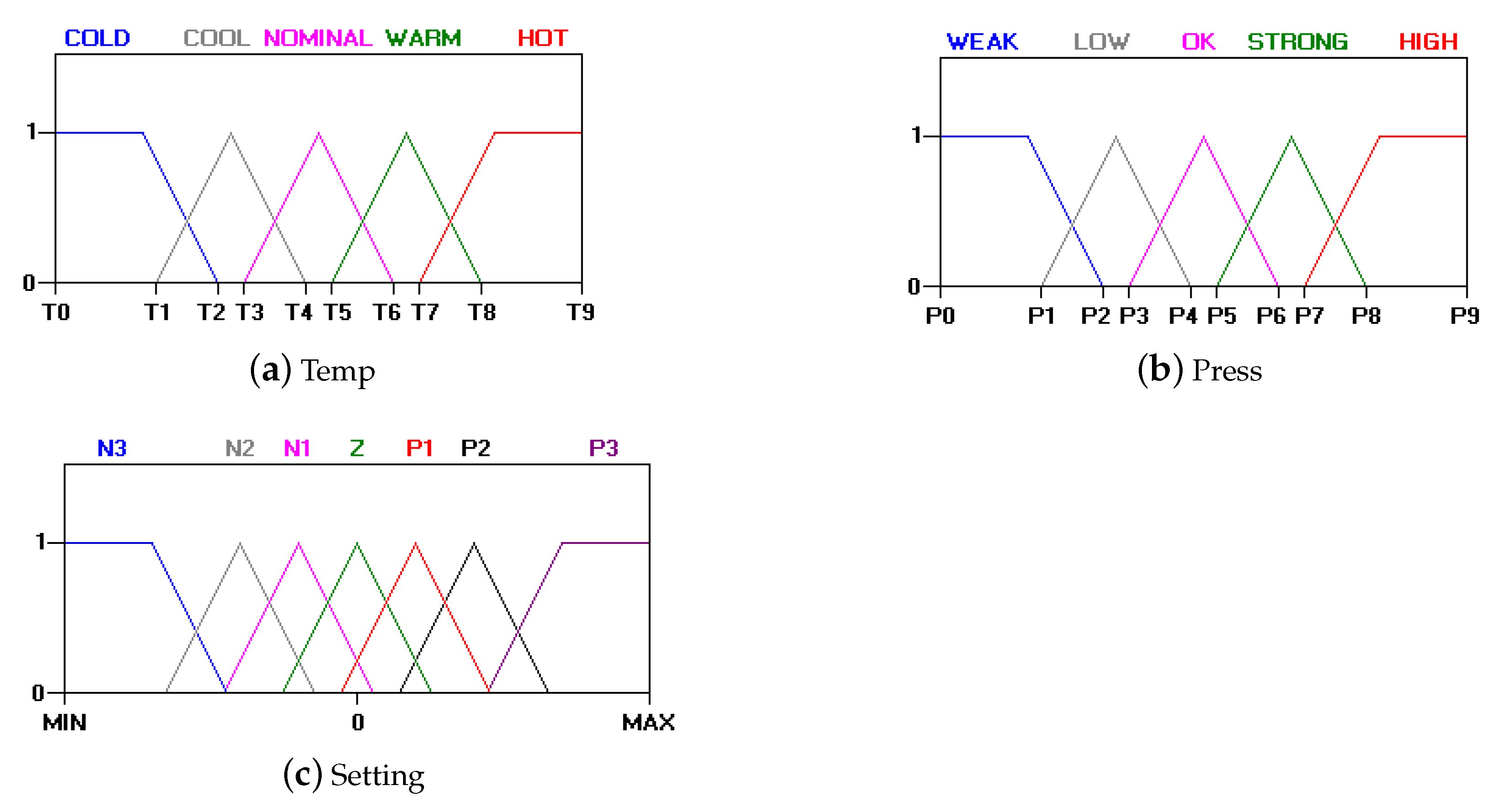
The system is composed of two fuzzification components $\mathsf{Temp},\mathsf{Press}$ and a defuzzification component $\mathsf{Setting}$ with corresponding membership functions illustrated in Figure 1. Note that $\Delta$ represents the copy operation.

In practice, the components $\mathsf{Temp}$ and $\mathsf{Press}$ execute in parallel. Each one will produce a membership value corresponding to the state and membership function after receiving a mode signal. After that, the minimum of the two output values will become the input of $\mathsf{Setting}$. The membership function of the $\mathsf{Setting}$ component is determined by the following rules (for simplicity, only whose conditions with temperature COOL are displayed).

$$\begin{array}{cc}\mathtt{rule}\mathtt{1}:\hfill & \mathtt{If}\mathtt{temperature}\mathtt{is}\mathtt{COOL}\mathtt{and}\mathtt{pressure}\mathtt{is}\mathtt{WEAK}\mathtt{then}\mathtt{throttle}\mathtt{is}\mathtt{P}\mathtt{3}.\hfill \\ \mathtt{rule}\mathtt{2}:\hfill & \mathtt{If}\mathtt{temperature}\mathtt{is}\mathtt{COOL}\mathtt{and}\mathtt{pressure}\mathtt{is}\mathtt{LOW}\mathtt{then}\mathtt{throttle}\mathtt{is}\mathtt{P}\mathtt{2}.\hfill \\ \mathtt{rule}\mathtt{3}:\hfill & \mathtt{If}\mathtt{temperature}\mathtt{is}\mathtt{COOL}\mathtt{and}\mathtt{pressure}\mathtt{is}\mathtt{OK}\mathtt{then}\mathtt{throttle}\mathtt{is}\mathtt{Z}.\hfill \\ \mathtt{rule}\mathtt{4}:\hfill & \mathtt{If}\mathtt{temperature}\mathtt{is}\mathtt{COOL}\mathtt{and}\mathtt{pressure}\mathtt{is}\mathtt{STRONG}\mathtt{then}\mathtt{throttle}\mathtt{is}\mathtt{N}\mathtt{2}.\hfill \\ \mathtt{rule}\mathtt{5}:\hfill & \mathtt{If}\mathtt{temperature}\mathtt{is}\mathtt{COOL}\mathtt{and}\mathtt{pressure}\mathtt{is}\mathtt{HIGH}\mathtt{then}\mathtt{throttle}\mathtt{is}\mathtt{N}\mathtt{3}.\hfill \\ \cdots \hfill \end{array}$$

The output functions are considered as non-fuzzy in this example.

(i)

The coalgebraic semantic of component $\mathsf{Temp}$

$$〚\mathsf{Temp}〛=(T,\theta \langle \overline{{\alpha }_t},\overline{e_t}\rangle ):T\to Z{(T\times [0,1])}^I)$$

is actually an $F_{I,[0,1]}$-coalgebra. In this model, states are the temperature over $T=[T_0,T_9]$, inputs are operation modes over set I = {COLD,COOL,NORMAL,WARM,HOT} that are decided by users. The fuzzy transition function is constant on the temperature and given by ${\alpha }_t:T\times I\to {[0,1]}^T$ with

$$\langle t,\mathtt{COLD}\rangle \mapsto {\varphi }_{COL},\langle t,\mathtt{COOL}\rangle \mapsto {\varphi }_{COO},\langle t,\mathtt{NORMAL}\rangle \mapsto {\varphi }_{NOR},\langle t,\mathtt{WARM}\rangle \mapsto {\varphi }_{WAR},\langle t,\mathtt{HOT}\rangle \mapsto {\varphi }_{HOT}$$

for all $t\in [T_0,T_9]\subseteq \mathbb{R}$. The output function $e_t:T\times I\to [0,1]$ is defined by $(t,i)\mapsto \mathsf{eval}({\alpha }_t(t,i),t)$ where $\mathsf{eval}$ is an evaluation function. As a concrete example, suppose the fuzzy subset for the NORMAL mode is the function

$${\varphi }_{NOR}(t)=max\{0,\frac{2}{T_3-T_6}(t-\frac{T_3+T_6}{2})+1\}.$$

Then the membership value (output) over state $\frac{T_3+T_6}{2}$ under the mode NORMAL is $e_t(\frac{T_3+T_6}{2},\mathtt{NORMAL})=\mathsf{eval}({\varphi }_{NOR},\frac{T_3+T_6}{2})=1$.

(ii)

$\mathsf{Press}$ is a component whose state space P is given by the pressure in the steam turbine and inputs are over the set $I^{\prime }=\{\mathtt{WEAK},\mathtt{LOW},\mathtt{OK},\mathtt{STRONG},\mathtt{HIGH}\}$, which represent the mode triggered by the users. The output of this component is the membership value corresponding to the current fuzzy state. The dynamics of this component is

$$〚\mathsf{Press}〛=(P,\theta \langle \overline{{\alpha }_p},\overline{e_p}\rangle ):P\to Z{(P\times [0,1])}^{I^{\prime }})$$

with the transition and output functions defined as ${\alpha }_p:P\times I^{\prime }\to Z(P)$:

$$\langle p,\mathtt{WEAK}\rangle \mapsto {\varphi }_{WEAK},\langle p,\mathtt{LOW}\rangle \mapsto {\varphi }_{LOW},\langle p,\mathtt{OK}\rangle \mapsto {\varphi }_{OK},\langle p,\mathtt{STRONG}\rangle \mapsto {\varphi }_{STRONG},\langle p,\mathtt{HIGH}\rangle \mapsto {\varphi }_{HIGH}$$

for $p\in P$ and

$$o_p:P\times I^{\prime }\to [0,1]:(p,i^{\prime })\mapsto \mathsf{ev}({\alpha }_p(p,i^{\prime }),p).$$

(iii)

The dynamics of $\mathsf{Rule}$ and $\mathsf{And}$ components are denoted by $⌜{\Psi }_1⌝$ and $⌜{\Psi }_2⌝$ where

$$⌜{\Psi }_1⌝=(\mathbf{1},\overline{{\eta }_{(\mathbf{1}\times O)}·\langle \mathsf{id},{\Psi }_1\rangle }:\mathbf{1}\to Z{(\mathbf{1}\times O)}^{I\times I^{\prime }}).$$

In this expression O is the output set determined by the output function, namely,

$${\Psi }_1:\mathbf{1}\times (I\times I^{\prime })\to O$$

$${\Psi }_1(\star ,(i,i^{\prime }))=\left\{\begin{array}{cc}\mathtt{P}\mathtt{3}\hfill & i=\mathtt{COOL}\wedge i^{\prime }=\mathtt{WEAK}\hfill \\ \mathtt{P}\mathtt{2}\hfill & i^{\prime }=\mathtt{COOL}\wedge \mathtt{LOW}\hfill \\ \mathtt{Z}\hfill & i^{\prime }=\mathtt{COOL}\wedge \mathtt{OK}\hfill \\ \mathtt{N}\mathtt{2}\hfill & i^{\prime }=\mathtt{COOL}\wedge \mathtt{STRONG}\hfill \\ \mathtt{N}\mathtt{3}\hfill & i^{\prime }=\mathtt{COOL}\wedge \mathtt{HIGH}\hfill \\ \cdots \hfill \end{array}\right.$$

$\mathbf{1}=\{\ast \}$ is the singleton set. The notation ⌜f⌝ is the representation of function $f:A\to B$, which is defined as a coalgebra $⌜f⌝=(\ast \in \mathbf{1},{\overline{c}}_{⌜f⌝})$, where $c_{⌜f⌝}=\mathbf{1}\times A\stackrel{\mathsf{id}\times f}{\to }\mathbf{1}\times B\stackrel{{\eta }_{(\mathbf{1}\times B)}}{\to }Z(\mathbf{1}\times B)$. The definition of ${\Psi }_2$ is similar, given a pair of inputs of $[0,1]$, it outputs the minimum value of the two.

(iv)

The last component $\mathsf{Setting}$ works as follows. Through the channel it interacts with $\mathsf{Temp}$ and $\mathsf{Press}$. It receives the mode information and a membership value as the current state. The mode information determines which membership function is accessible for the component. Then the component outputs an area whose boundary consists of the horizontal axis and the graph of the membership function. Formally, this model is represented by a coalgebra

$$〚\mathsf{Setting}〛=(D,\theta \langle \overline{{\alpha }_s},\overline{e_s}\rangle ):D\to Z{(D\times P({\mathbb{R}}^2))}^{O\times [0,1]})$$

where $D=[\mathtt{MIN},\mathtt{MAX}]$ is an interval of real numbers. The output function is defined as $e_s(d,(o,r))=\{(x,y)|0\le y\le min\{{\alpha }_s(x,(o,r)),r\},x\in [\mathtt{MIN},\mathtt{MAX}]\}$. Resorting to centroid defuzzification technique, the output stage processes combine areas and produce a control value, which will participate in the control of the system.

7. Conclusions and Future Work

The present work aims at addressing fuzzy automata from a coalgebraic perspective. Our starting point was studying the fuzzy-set monad further. We defined a left tensorial strength and a right tensorial strength, and proved it is a strong and commutative monad. With these properties, we modeled different types of fuzzy automata as coalgebraic models with the same transition structure. Based on these coalgebraic models, we defined the notions of fuzzy language bisimulation between fuzzy automata. Moreover, we developed some compositional combinators for fuzzy Mealy automata of two kinds: state transition and output function and compared it with the classical component calculi in [32]. Finally, through a case study, we discussed the application of our component calculi.

Besides these fundamental results, there are several topics left to explore. One is to define a notion of refinement [38] of fuzzy automata, to specify an inclusion relation of fuzzy behaviour. Fuzzy automata may involve complex behaviour such as non-deterministic transitions or branched transitions with probability [23,39]. Therefore another topic for future work is to develop more complex versions of fuzzy automata and analyze their behavior and discuss their properties, namely of the suitable notions of bisimulation as in [15,35,36].

References

- Tanaka, K. An Introduction to Fuzzy Logic for Practical Applications; Springer: Berlin/Heidelberg, Germany, 1997. [Google Scholar]
- Zadeh, L.A. Soft Computing and Fuzzy Logic. IEEE Softw. 1994, 11, 48–56. [Google Scholar] [CrossRef]
- Syropoulos, A.; Grammenos, T. Fuzzy Computation; A Modern Introduction to Fuzzy Mathematics; John Wiley & Sons: Hoboken, NJ, USA, 2020; pp. 191–214. [Google Scholar] [CrossRef]
- Wu, H.; Gu, X.; Zhen, L. Fuzzy Principal Component Analysis Model on Evaluating Innovation Service Capability. Sci. Program. 2020, 2020, 8834901. [Google Scholar] [CrossRef]
- Böhme, M.; Pham, V.; Roychoudhury, A. Coverage-Based Greybox Fuzzing as Markov Chain. IEEE Trans. Softw. Eng. 2019, 45, 489–506. [Google Scholar] [CrossRef]
- Simon, D.J. Introduction to Fuzzy Control. In Embedded Systems Programming; Electrical Engineering & Computer Science Faculty Publications: Cambridge, MA, USA, 2003; Volume 16, pp. 55–56. [Google Scholar]
- Doostfatemeh, M.; Kremer, S.C. New directions in fuzzy automata. Int. J. Approx. Reason. 2005, 38, 175–214. [Google Scholar] [CrossRef] [Green Version]
- Chaudhari, S.R.; Desai, A.S. On fuzzy Mealy and Moore machines. Bull. Pure Appl. Math 2010, 4, 375–384. [Google Scholar]
- Mordeson, J.N.; Nair, P.S. Fuzzy Mealy machines. Kybernetes 1966, 25, 18–33. [Google Scholar] [CrossRef]
- Li, Y.; Pedrycz, W. The equivalence between fuzzy Mealy and fuzzy Moore machines. Soft Comput. 2006, 10, 953–959. [Google Scholar] [CrossRef]
- Todinca, D.; Sora, I.; Butoianu, D.; Precup, R. A Novel Method to Compute the Membership Value of the States of Fuzzy Automata. In Proceedings of the 2018 IEEE 12th International Symposium on Applied Computational Intelligence and Informatics (SACI), Timisoara, Romania, 17–19 May 2018; pp. 107–112. [Google Scholar] [CrossRef]
- Pan, H.; Li, Y.; Cao, Y.; Li, P. Nondeterministic fuzzy automata with membership values in complete residuated lattices. Int. J. Approx. Reason. 2017, 82, 22–38. [Google Scholar] [CrossRef]
- Tiwari, S.P.; Pal, P. On a category of deterministic fuzzy automata. In 11th Conference of the European Society for Fuzzy Logic and Technology (EUSFLAT 2019); Atlantis Studies in Uncertainty Modelling; Atlantis Press: Paris, France, 2019; Volume 1. [Google Scholar] [CrossRef]
- Mockor, J. Monads and a common framework for fuzzy type automata. Int. J. Gen. Syst. 2019, 48, 406–442. [Google Scholar] [CrossRef]
- Singh, A.K.; Tiwari, S.P. Fuzzy Regular Languages Based on Residuated Lattice. New Math. Nat. Comput. 2020, 16, 363–376. [Google Scholar] [CrossRef]
- Yang, C.; Li, Y. Approximate bisimulations and state reduction of fuzzy automata under fuzzy similarity measures. Fuzzy Sets Syst. 2020, 391, 72–95. [Google Scholar] [CrossRef]
- Yang, C.; Li, Y. ϵ-Bisimulation Relations for Fuzzy Automata. IEEE Trans. Fuzzy Syst. 2018, 26, 2017–2029. [Google Scholar] [CrossRef]
- Yang, C.; Li, Y. Approximate bisimulation relations for fuzzy automata. Soft Comput. 2018, 22, 4535–4547. [Google Scholar] [CrossRef]
- Rutten, J.J.M.M. Automata and coinduction (an exercise in coalgebra). In International Conference on Concurrency Theory, Proceedings of the CONCUR 1998: CONCUR’98 Concurrency Theory, Nice, France, 8–11 September 1998; Springer: Berlin/Heidelberg, Germany, 1998; Volume 1466, pp. 194–218. [Google Scholar]
- Rutten, J.J.M.M. Universal coalgebra: A theory of systems. Theor. Comput. Sci. 2000, 249, 3–80. [Google Scholar] [CrossRef] [Green Version]
- Jacobs, B. Introduction to Coalgebra: Towards Mathematics of States and Observation; Cambridge Tracts in Theoretical Computer Science; Cambridge University Press: Cambridge, UK, 2016; Volume 59. [Google Scholar]
- Silva, A.; Bonchi, F.; Bonsangue, M.M.; Rutten, J.J.M.M. Generalizing determinization from automata to coalgebras. Log. Methods Comput. Sci. 2013, 9. [Google Scholar] [CrossRef] [Green Version]
- Sokolova, A. Coalgebraic Analysis of Probabilistic Systems. Ph.D. Thesis, Technische Universiteit Eindhoven, Eindhoven, The Netherlands, 2005. [Google Scholar]
- Neves, R.; Barbosa, L.S. Hybrid Automata as Coalgebras. In International Colloquium on Theoretical Aspects of Computing, Proceedings of the ICTAC 2016: Theoretical Aspects of Computing, Taipei, Taiwan, 24–31 October 2016; Lecture Notes in Computer Science; Springer: Berlin/Heidelberg, Germany, 2016; Volume 9965, pp. 385–402. [Google Scholar] [CrossRef] [Green Version]
- Neves, R.; Barbosa, L.S. Languages and models for hybrid automata: A coalgebraic perspective. Theor. Comput. Sci. 2018, 744, 113–142. [Google Scholar] [CrossRef]
- Liu, A.; Sun, M. A Coalgebraic Semantics Framework for Quantum Systems. In International Conference on Formal Engineering Methods, Proceedings of the ICFEM 2019: Formal Methods and Software Engineering, Shenzhen, China, 5–9 November 2019; Lecture Notes in Computer Science; Springer: Berlin/Heidelberg, Germany, 2019; Volume 11852, pp. 387–402. [Google Scholar] [CrossRef]
- Feng, Y.; Duan, R.; Ying, M. Bisimulation for Quantum Processes. ACM Trans. Program. Lang. Syst. 2012, 34, 1–43. [Google Scholar] [CrossRef] [Green Version]
- Larsen, K.G.; Skou, A. Bisimulation through probabilistic testing. Inf. Comput. 1991, 94, 1–28. [Google Scholar] [CrossRef] [Green Version]
- Haghverdi, E.; Tabuada, P.; Pappas, G.J. Bisimulation Relations for Dynamical and Control Systems. Electr. Notes Theor. Comput. Sci. 2002, 69, 120–136. [Google Scholar] [CrossRef] [Green Version]
- Jacobs, B. Invariants, Bisimulations and the Correctness of Coalgebraic Refinements. In International Conference on Algebraic Methodology and Software Technology, Proceedings of the AMAST 1997: Algebraic Methodology and Software Technology, Sydney, Australia, 13–17 December 1997; Lecture Notes in Computer Science; Springer: Berlin/Heidelberg, Germany, 1997; Volume 1349, pp. 276–291. [Google Scholar] [CrossRef]
- Venema, Y. Algebras and coalgebras. In Handbook of Modal Logic; Studies in Logic and Practical Reasoning; Elsevier B.V.: Amsterdam, The Netherlands, 2007; Volume 3, pp. 331–426. [Google Scholar] [CrossRef] [Green Version]
- Barbosa, L.S. Components as Coalgebras. Ph.D. Thesis, Universidade do Minho, Braga, Portugal, 2001. [Google Scholar]
- Guilherme, R.J.P. A Coalgebraic Approach to Fuzzy Automata. Ph.D. Thesis, Universidade Nova De Lisboa, Lisbon, Portugal, 2016. [Google Scholar]
- Wu, H.; Chen, Y. Coalgebras for Fuzzy Transition Systems. Electron. Notes Theor. Comput. Sci. 2014, 301, 91–101. [Google Scholar] [CrossRef] [Green Version]
- Wu, H.; Chen, Y.; Bu, T.; Deng, Y. Algorithmic and logical characterizations of bisimulations for non-deterministic fuzzy transition systems. Fuzzy Sets Syst. 2018, 333, 106–123. [Google Scholar] [CrossRef]
- Wu, H.; Chen, T.; Han, T.; Chen, Y. Bisimulations for fuzzy transition systems revisited. Int. J. Approx. Reason. 2018, 99, 1–11. [Google Scholar] [CrossRef] [Green Version]
- Nikravesh, M.; Kacprzyk, J.; Zadeh, L.A. Forging New Frontiers: Fuzzy Pioneers I; University of California: Berkeley, CA, USA, 2007. [Google Scholar]
- Meng, S.; Barbosa, L.S. Components as coalgebras: The refinement dimension. Theor. Comput. Sci. 2006, 351, 276–294. [Google Scholar] [CrossRef] [Green Version]
- Narasimha, M.; Cleaveland, R.; Iyer, S.P. The role of observations in probabilistic open systems. Electr. Notes Theor. Comput. Sci. 1999, 25, 133–144. [Google Scholar] [CrossRef] [Green Version]
Figure 1.
The graphs of membership functions.
Publisher’s Note: MDPI stays neutral with regard to jurisdictional claims in published maps and institutional affiliations. |
© 2021 by the authors. Licensee MDPI, Basel, Switzerland. This article is an open access article distributed under the terms and conditions of the Creative Commons Attribution (CC BY) license (http://creativecommons.org/licenses/by/4.0/).
Share and Cite
MDPI and ACS Style
Liu, A.; Wang, S.; Barbosa, L.S.; Sun, M. Fuzzy Automata as Coalgebras. Mathematics 2021, 9, 272. https://0-doi-org.brum.beds.ac.uk/10.3390/math9030272
AMA Style
Liu A, Wang S, Barbosa LS, Sun M. Fuzzy Automata as Coalgebras. Mathematics. 2021; 9(3):272. https://0-doi-org.brum.beds.ac.uk/10.3390/math9030272
Chicago/Turabian StyleLiu, Ai, Shun Wang, Luis Soares Barbosa, and Meng Sun. 2021. "Fuzzy Automata as Coalgebras" Mathematics 9, no. 3: 272. https://0-doi-org.brum.beds.ac.uk/10.3390/math9030272
Note that from the first issue of 2016, this journal uses article numbers instead of page numbers. See further details here.