Accurate Prediction of Concentration Changes in Ozone as an Air Pollutant by Multiple Linear Regression and Artificial Neural Networks

Abstract

This study considers the usage of multilinear regression and artificial neural network modelling to forecast ozone concentrations with regard to weather-related indicators (wind speed, wind direction, relative humidity and temperature). Initial data were obtained by measuring the meteorological parameters using the PC Radio Weather Station. Ozone concentrations near high-voltage lines were measured using RS1003 and at a 220 m distance using ML9811. Neural network models such as the multilayer perceptron and radial basis function neural networks were constructed. The prognostic capacities of the designed models were assessed by comparing the result data by way of the square of the coefficient of multiple correlations (R²) and mean square error (MSE) values. The number of hidden neurons was optimised by decreasing an error function that recorded the number of units in the hidden layers to the precision of the expanded networks. The neural software IBM SPSS 26v was used for artificial neural network (ANN) modelling. The study demonstrated that the linear regression modelling approach was lacking in its capacity to predict the investigated ozone concentrations by used parameters, whereas the use of an ANN offered more precise outcomes. The conducted tests’ results established the strength of the designed artificial neural network models with irrelevant differences between detected and forecasted data.

1. Introduction

High-voltage power transmission powerlines lead to the formation of strong electric and magnetic fields nearby. The effect of these fields that are close to the 300 kV powerlines covers a distance of up to approximately 200 m [1]. Moreover, the level of noise near the high-voltage power transmission lines is 1.5 times higher than that in the analogous territories without powerlines, reaching 50–55 dBA.

The studies carried out in the United Kingdom and Europe show that all high-voltage power transmission lines are surrounded by a corona of ions. A greater corona is observed with older powerlines that have rougher surfaces [2,3,4]. Corona ions carried downwind of the lines attach themselves to up to 15,000 pollution particles per cubic metre floating in the air [5,6,7].

The ground-level ozone exists as a natural atmospheric impurity. The increase in the levels of ozone is determined by natural and artificial sources of ozone formation. Ozone usually forms in the atmosphere during discharges—e.g., lightning or corona discharge near the transmission lines of high-voltage power (HVP). Therefore, HVp transmission lines may be considered a significant source of air pollution by way of ozone and nitrogen oxides. In the surroundings of high-voltage power transmission lines, the formation of hydroxyl radicals (OH) that promote oxidation of volatile organic compounds and cause changes in air composition is also observed [2].

The research carried out by Elansky et al. [4] has revealed that the ozone levels near the 220 kV powerlines are 2 ppb higher than the levels in the areas away from the powerlines, and 3 ppb higher near the 500 kV powerlines, respectively. These scientists have found that the ozone levels that form near the high-voltage power transmission lines comprise 0.1% of all levels of ozone forming in the troposphere during photochemical processes.

The effects of high-voltage power transmission lines may cause humans to suffer from changes in the function of their cardiovascular, respiratory and immune systems, as well as other health problems [8,9,10,11]. The human body is live antenna that can assimilate and re-emit [8] the energy of powerlines in the environment. Electromagnetic fields pose a higher risk to developing bodies—e.g., children [7,8,9,10]. Swedish scientists have found that the children living in close proximity to powerlines are exposed to a 2–5 times higher risk of leukaemia. In 2005, researchers at Oxford University proved a high risk (69%) of leukaemia in children who live within 200 m of HVP lines from birth and for children living within a distance from 200 to 599 m, this risk was identified at 23%, which is the risk also associated with those who live farther than 600 m away from powerlines from birth [11]. The cumulative impact of ozone and aerosol particles on human nose, throat and eyes is significantly stronger than that of each pollutant separately. Therefore, this research analyses the dynamics of both the ozone levels and aerosol particles in the surroundings of high-voltage powerlines.

Magnetic and electric fields forming close to powerlines have been widely researched. However, little is known about ozone formation in the surroundings of high-voltage powerlines. Therefore, it is important to determine the role of high-voltage powerlines in the formation of ground-level ozone and the influence of meteorological conditions on the intense formation of ozone in the researched area.

The aim of the research was to design prediction models that may be used to predict the precision of the peculiarities of the ozone concentration changes near high-voltage transmission powerlines by applying different methods such as multiple linear regression and an artificial neural network. It also aimed to evaluate the effect of environmental parameters on the changes of this pollutant close to the area of the source of the manmade ozone.

Not only experimental but also modelling research on distribution of pollutants near little-studied objects such as high-voltage power transmission lines has been carried out. By taking into consideration meteorological conditions, the new and important tool intended not only for analysis but also for predicting pollution dynamics and potentially for solving specific environmental pollution problems has been developed.

The study is presented in sections as follows: Section 2 considers prediction of pollution by employing an artificial neural network (ANN); the methodology for analysing the data of the study is presented in Section 3; Section 4 discusses the collection of the experimental data and the characteristics of the analysers used; in Section 5 are presented the conducted data analysis and the results; the discussions according to the results of the analysis and the limitations of the research are in presented in Section 6; Section 7 proposes conclusions and future research directions.

2. ANN in Predicting Air Pollution

At present, air pollution is considered to be a severe environmental hazard in the world as it can cause an increase in severe respiratory and cardiovascular illnesses, as well as changes in environmental conditions [12]. Recently, this problem has drawn the attention of scholars due to its high effect on human health. It has influenced municipal supervisors to implement air pollution monitoring measures [13,14,15,16]. Nevertheless, the temporary monitoring of air quality alone cannot meet all the requirements. Consequently, designing a precise and reliable model is vital in predicting air pollution as it could be used to detect air pollution in its early stages, thus avoiding its harmful effects on the environment and health by way of proper control measures [12].

The increase in air pollution is influenced by factors such as the types of pollutants and the meteorological conditions in the area [12,13,14,15,16]. In this case, the meteorological conditions and constraints are among the controlling factors for the transfer and spread of the air pollutants in the area [12]. Therefore, applying the constructed models to the collected data may produce valuable results. Current findings prove that meteorological conditions play a key role in the daily volatility of the air pollutant concentrations [12,13,14,15,16].

Lately, a substantial amount of research has been focused on predicting air pollution with the aim to form and develop models using meteorological data, including statistical models, the community multiscale air quality model and research and prediction models using chemistry, neuro-fuzzy inference systems, and other similar models [17,18,19,20]. Out of these types of analytical models, the artificial neural network has provided the most significant results and therefore is widely used in the predictive areas. Recently, a variety of the artificial neural network structures have been established to expand their predictive functions as to the air pollutant concentrations, and several studies have been conducted in this regard [17,18,19,20]. Several models using ANNs were constructed to predict the ozone concentration in an area. They included meteorological parameters as the input variables [21]. According to the findings of Gao et al. [21], the ANN model could offer a precise forecast of the ozone levels in an environment. Paschalidou et al. [22] presented results of their study which demonstrated the main predicting variables significantly affecting the precision of ozone level predictions in an environment to be the following: maximum temperature, atmospheric pressure, period of sunlight and the maximum wind speed [22].

Identifying and forecasting air pollution is vital for the purposes of advanced detection and control before the situation develops into an air pollution event. The present study aimed to optimise and evaluate the combined ANN methods for the modelling and prediction of the changes in the ozone concentration levels near high-voltage power transmission lines. It also aimed to measure the influence of the environmental conditions on the changes of this pollutant close to area of the manmade ozone source in order to produce an effective tool for predicting air pollution.

3. Methodology for Analysing the Data of the Study

The analysis in the study was performed by employing the two different analyses. The first was a multiple linear regression (MLR) [. Additionally, artificial neural network (ANN) modelling was used to predict the peculiarities of the changes in the ozone concentration levels near high-voltage power transmission lines, measured by RS1003 (RS); ozone concentration was measured by the ML9811 sensor at a distance of 220 m (ML); aerosol particles (ASs) were measured in 10⁶/m³; temperature (TE) was measured in °C; humidity (HU) was measured in percentage; wind speed (WS) was measured in m/s; wind direction (WD) was measured in degrees; atmospheric pressure (PR) was measured in mmHg.

An experimental study was conducted to gather the real situation regarding ozone concentrations. Three multiple linear regression models were constructed to analyse the experimental data sample: for the dependent variable RS—Model 1, for dependent variable ML—Model 2 and Model 3, because ML and as additional parameter was included in RS. To predict the peculiarities of the changes in the ozone concentration levels near a high-voltage power transmission line such as regressors (input parameters), in these models ASs, TE, HU, WS, WD and PR were used.

Additionally, neural network models such as the multilayer perceptron (MLP) and the radial basis function (RBF) were constructed. The analytical capacities of designed models were assessed by comparing the result data by way of the determination coefficient (R²) and the mean square error (MSE) measures. The constructions of the MLP and RBF neural networks were not complicated, involving only one hidden layer. The number of units in the hidden layers was optimised by reducing an error function that recorded the number of hidden nodes to the precision of extended networks. The IBM SPSS 26v software was used for the ANN modelling. Collected data were categorised into three portions: training, testing and holdout.

Seven independent continuous variables were used as inputs and one for output in the network, corresponding to environment components and ozone concentrations, respectively. The hidden neurons were optimised by building various MLP and RBF ANNs with 5–50 hidden nodes.

The network training was carried out with the objective function that can be explained as the sum of square errors, and it evaluated the difference between the measured value for the ozone concentration level and the value predicted by the model in each spatial point. In this case, a part of experimental data was chosen for training, using the least squares metric. The designed neural network was validated through calculations, comparing predictions with the collected set of experimental data.

3.1. Multiple Linear Regression

Multiple linear regression (MLR) methods based on least-square dealings are regularly used for assessing the variable effects involved in a model [23,24,25]. In this study, three MLR models were accepted for the collected experimental data. Ozone concentration was used as the response variables in these models. Model 1 was designed to predict the ozone concentration near high-voltage powerlines measured by RS 1003 (dependent variable RS, Model 1, Table 5); Model 2—ozone concentration was measured by ML9811 at a distance of 220 m (ML, Model 2, Table 5) with six aspects; Model 3 (ML, Table 5) was measured with seven aspects as prognosticator variables. In the constructed models, the responses for ozone concentrations were expressed as functions of the six environmental parameters in order to explain and assess the impacts on the changes of ozone levels as pollutant concentrations. The accuracies of the constructed MLR models were estimated by assessing the degree of the determination coefficient R², the residual standard error (RSE) for the regression and the Student’s t-test outcomes for the separate predictor variables.

3.2. Artificial Neural Networks

ANNs are a category of artificial intelligence that are constructed based on the brain’s neural operations [25]. A neural network is composed of elements that process simultaneously—i.e., neurons [26]. The ANNs are typically comprised of three layers—the first is the input layer, the second is the hidden layer, and the third is the output layer—which connect the inputs units to the outputs. The choosing of the input parameters is the main aspect of neural network modelling [27]. The number of neurons in the hidden layer depends on the features of the problem being investigated. The training dataset is useful to teach the ANN to find the global all-inclusive model between its input variables and outputs. The MLP and the RBF neural network structures were employed in this study to make accurate predictions on the influence of the meteorological conditions and the high-voltage powerlines on ground-level ozone formation. The nonlinear efficiencies of ANNs renders them good estimators that are capable of providing very accurate results.

3.2.1. The Architecture of the Multilayer Perceptron Neural Network

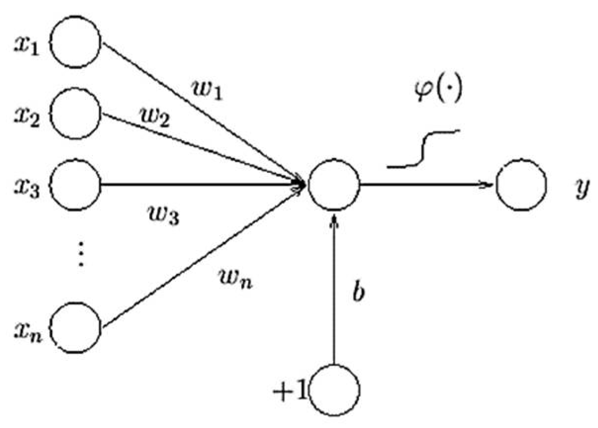
A multilayer perceptron network can be presented as a network of simple neurons named perceptrons. The first form of a single perceptron was presented in 1958 [28]. To explain the conception of MLP, one has to start from the explanation of one perceptron, and then to the possibility of computing a single output from multiple real-valued inputs by forming a linear combination according to its input weights and then possibly putting the output through some nonlinear activation function. Scientifically, this can be explained by the following equation:

$$y=\phi \left({\displaystyle \sum }_{i=1}^n{w}_i·x_i+b\right)=\phi \left(W^T·X+b\right)$$

(1)

where w represents the vector of weights, X is the vector of inputs, b is the bias and φ is the activation function. Figure 1 represents the signal-flow operation in the graphical view [29,30,31].

Regardless of the activation function chosen, the perceptron can only represent an oriented ridge-like function. Typically, the MLP network contains of a set of basis nodes establishing the input layer, then one or more hidden layers of computation nodes are included, and an output layer of nodes. The ANN’s single hidden layer with nonlinear activation functions and a linear output layer can be explained by the following equation:

$$X=f\left(s\right)=B·\phi \left(A·s+a\right)+b,$$

(2)

where s is a vector of inputs and X is a vector of outputs. A is the matrix of weights of the first layer and a is the bias vector of the first layer. B and b are the weight matrix and the bias vector of the second layer, respectively. The function φ represents an elementwise nonlinearity.

IBM SPSS 26v software as the activation function for the MLP networks design has a sigmoid function that is a logistic function and can be defined by the following equation:

$$S\left(x\right)=\frac{1}{1+e^{-x}}=\frac{e^x}{e^x+1}$$

(3)

The other MLP activation function can be a hyperbolic tangent:

$$f\left(x\right)=\tan \mathrm{h}\left(x\right)=\frac{e^x-e^{-x}}{e^x+e^x}$$

(4)

This is a shifted and scaled version of the logistic function presented in Equation (3).

Functions such as the sigmoid function most often show a return value for the y axis (dependent variable values) in the interval of 0 to 1 (Equation (3)), or they can range from −1 to 1 (Equation (4)). The relationship between these functions can be described by the following equation:

$$f\left(x\right)=\frac{\tanh \left(x\right)+1}{2}=\frac{1}{1+e^{-2x}}.$$

(5)

The functions above ((3) and (4)) were chosen because they are scientifically appropriate and are close to linear near the origin while saturating rather quickly when moving away from the source. As mentioned above, MLP networks are able to model both strong and mild nonlinear mappings well.

3.2.2. Architectures of the Radial Basis Function (RBF) Neural Network

The architectures of the radial basis function (RBF) neural network are feasibly the most frequently used ANNs [28,29,30,31,32,33,34]. The RBF neural network typically involves three layers: the input layer, the hidden layer and the output layer. The inputs of the hidden layer can be introduced as the linear mixtures of scalar weights and the input vector, where the scalar weights are usually allocated as unit values—that is, the whole input vector appears to each neuron in the hidden layer. The inbounding vectors are mapped by the radial basis functions in each hidden node. The output layer produces a vector by linear combination of the outputs of the hidden nodes to yield the final output [30,33,34]. The construction of an n inputs and m outputs RBF neural network can be explained by the following equation:

$$y=f_j\left(k\right)={{\displaystyle \sum }}_{i=1}^n{w}_j^i{\phi }_i\left(k\right),forj=1,\dots , m,$$

(6)

where k = {k₁, k₂,…,k_n} denotes the input vector for n inputs and y = {y₁, y₂,…,y_m} represents the output vector for 𝑚 outputs; $w_j^i$ represents the weight of the ith hidden nodes and the jth output node and n is the total number of hidden nodes; ${\phi }_i$(⋅) denotes the RBF of the ith hidden node. The linear combination of all hidden nodes presents the final output of the jth output node (k). Later, as the denominator is used for the summation, Equation (5) can be normalised by the following equation:

$$y=f_j\left(k\right)=\frac{{{\displaystyle \sum }}_{i=1}^n{w}_j^i{\phi }_i\left(k\right)}{{{\displaystyle \sum }}_{i=1}^p{\phi }_i\left(k\right)},for j=1,\dots , m.$$

(7)

The distance between a given input vector and a predefined centre vector is describing the multidimensional function RBF, and can be specified by the following equation:

$${\phi }_i\left(k\right)=exp\left(-\frac{||k-\mu {||}^2}{2{\sigma }_i^2}\right),for i=1,\dots , p.$$

(8)

The expanded RBF network included a softmax function in this study. The softmax function can be described by the following equation:

$$\sigma \left(z\right)j=\frac{\tanh \left(x\right)+1}{{{\displaystyle \sum }}_{k=1ezk}^{k}x}, for j=1,\cdots , k.$$

(9)

The softmax function used in this study was used to manage multiple classes alone, when one class in other activation functions normalises the yields for each class between 0 and 1, and divides by their sum, giving the probability of an input value being in a specific class.

It has been argued that an ANN with a single hidden layer and sufficient data can be used to model any function [30]. Consequently, the MLP or RBF neural network structures used contained only one hidden layer. Accordingly, constructing the ANN requires choosing a satisfactory number of hidden neurons and appropriate network organisations in concordance with the specifical and nature of inputs (e.g., discrete variables, continuous, categorical, or quantitative). The quantity of hidden neurons was optimised by decreasing an error function that mapped the number of nodes in the hidden layer to the precision of the extended networks.

The modelling of the designed ANNs was carried out by IBM SPSS 26v software. The data of the study were categorised into three parts: training, testing and holdout. For the network modelling, seven independent variables were used as inputs and one variable as output variable, corresponding to the description of environment conditions and ozone concentration. The various MLPs and RBFs were built with hidden nodes of 5–50 t to optimise the designed ANNs. The investigations for networks with hidden nodes greater than 50 were not continued due to the predictive capabilities decreasing with the number of intermediate units. The selection of the best model was carried out taking into account the determination coefficient and the mean square error (MSE) measures. The mean square error (MSE) and the determination coefficient (R²) are the standard criteria for the estimation of statistical performance and are used to assess the precision of the predictive capacity of the designed models. Accordingly, the goodness of fit in these investigations is established by mean squared error (MSE), which can be explained by the following equation:

$$MSE=\frac{1}{ns}{\displaystyle \sum }_{j=1}^n{\displaystyle \sum }_{i=1}^s{\left(Y_{j,i}-y_{j,i}\right)}^2,$$

(10)

where Y_j,i is the consummate value of jth data sample at ith data output and y_j,i is the actual value of jth data sample at ith data output; n is the quantity of samples and s is the number of neurons at the output layer. The dissimilar mixtures of activation functions and neuron quantities were assessed by identifying the fitted model, taking into account the MSE.

4. Methodology of Collecting the Experimental Data

The experiment was carried out in autumn in the eastern part of Lithuania in an area close to two 330 kV high-voltage powerlines. The research was conducted for a period of 120 h by recording the levels of ozone and the aerosol particles together with meteorological parameters every 5 min. The RS1003 and ML9811 analysers were used to measure ozone concentrations, the AZ-5 sensor was used to measure the aerosol particles and the meteorological weather station, PC Radio Weather Station, was used to record the environmental factors.

4.1. Analysers Used for Collecting the Experimental Data

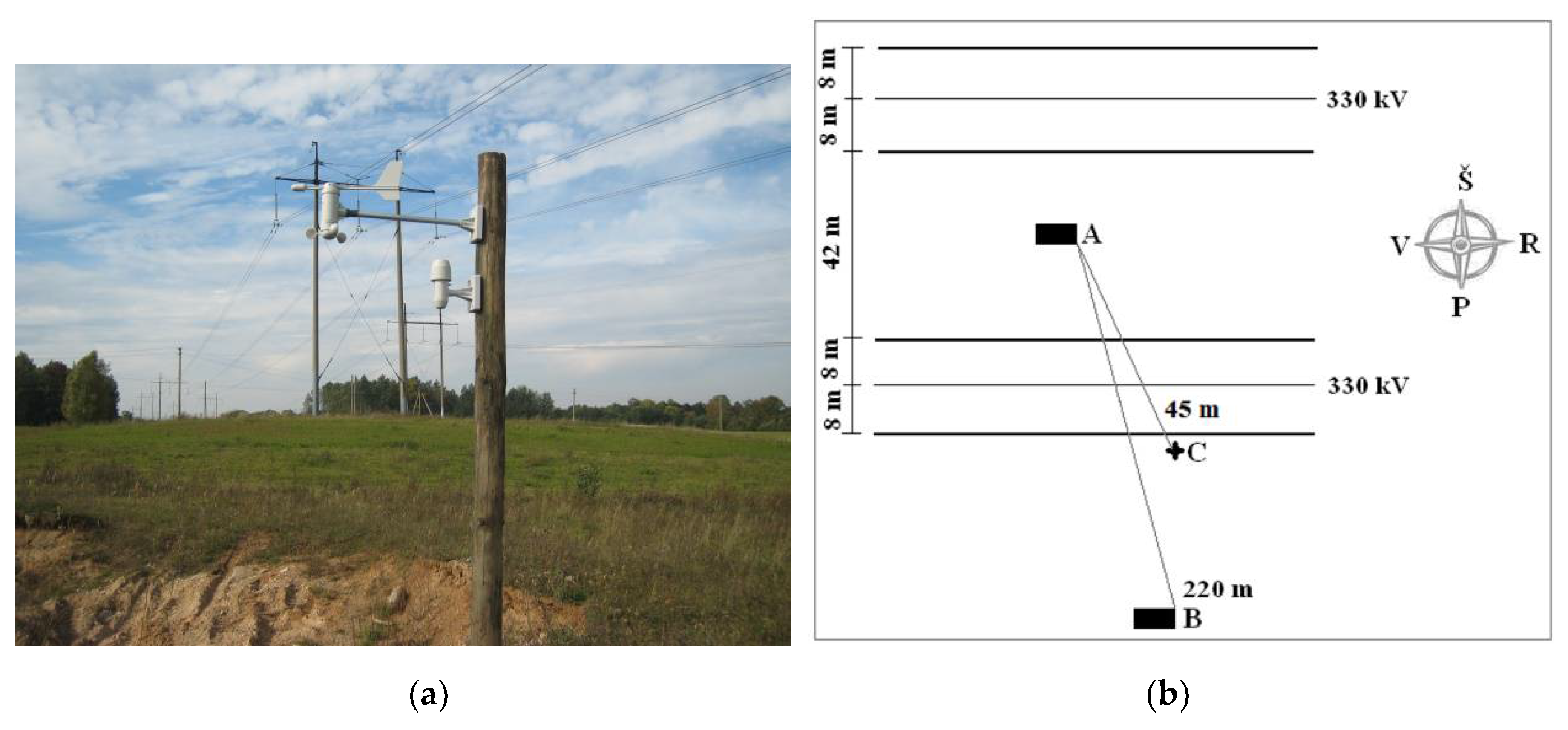
Ozone concentrations near the high-voltage powerlines were measured with the RS1003 ozone analyser, while the ML9811 analyser was used to measure the “background” levels of ozone at a 220 m distance from the powerlines. Technical specifications of the ozone analysers are presented in the

Table 1. Technical specifications of the ozone analysers.

Specifications	RS1003	ML9811
Mode	0–1000 ppb	0–2000 ppb
Measurement Range	0.5 ppb	0.5 ppb
Detection limit	1%	1%
Linearity	1.0 L/min	1.6 L/min
Sample flow rate	0–45 °C	0–45 °C
Standard operating temperature
Weight	10 kg	16 kg

. The detailed scheme of locations for measuring ozone concentrations are shown in Figure 2.

The 1003RS and ML9811 ozone analysers were calibrated before the experiment. After calibration, both analysers operated for several days by pulling the air samples through a tube from the same spot. The coefficient found between both analysers was 0.997.

The sensitivities of these ozone analysers are 1 ppb and they function within a wide range of temperatures—i.e., from 0 to 45 °C. During the experiment, the numerical concentrations of 0.4 μm aerosol particles were measured with the AZ-5 sensor with the measurement tolerance not exceeding 20% (the location of the sensor was the same as square A in Figure 2b). The technical parameters of the AZ-5 sensor are detailed in

Table A6. Technical specifications of aerosol particles counter.

Model AZ-5
Parameters Measured	Measurement Values
Particle size	0.4; 0,5; 0.6; 0.7; 0.8; 0.9; 1,0; 1.5; 2.0; 4.0; 7.0; 10.0 μm
Temperature range	+10 °C to +35 °C
Measuring range, atmospheric pressure	750 ± 30 mmHg
Sample flow rate	1.2 l/min

(see Appendix B). The concentrations of ozone and aerosol particles were measured by using a teflon tube for air intake at the height of 1.5 m from the ground. The levels of both the ozone and the aerosol particles were continuously measured by recording the average values of the pollutants on the computer database every 5 min. The analogue signal was converted into a digital one by using the ADC-16 data logger. The data were collected and analysed by using the PicoLog software.

During the research period, the meteorological parameters such as air temperature, relative humidity in the air, atmospheric pressure and the speed and direction of wind were measured continuously. These parameters were measured using the weather station (PC Radio Weather Station) by way of receiving the signal via radio waves from the sensors of the weather station attached to a pillar that was located 45 m southeast from the ozone analyser and the aerosol particle metre. This weather station operates within a wide range of temperatures (from −30 to +70 °C), relative humidity values in the air (from 20% to 100%), and wind speeds (from 0 to 65 m/s). In order to carry out the data analysis, the wind direction was categorised into 8 parts, each representing forty-five degrees. The data were automatically recorded on a computer every 5 min.

4.2. Sample Variables Description

The knowledge on ozone formation in the surroundings of high-voltage powerlines and the influence of environmental conditions on the changes of this pollutant close to a manmade ozone source has been limited. In this study, we investigated the peculiarities of the variations in ozone concentration levels near HVP transmission lines (variable RS) and the levels at a distance of 220 m (variable ML) by employing different ozone analysers. Additionally, we measured several meteorological parameters, including AS, TE, HU, WS, WD and PR which were used as independent variables in the conducted analysis. A detailed explanation of the variables involved in the study is presented below. The independent variables were measured by specifical devices which are validated for these type environment conditions evaluation. All collected data are parametric, and was collected to investigate and to weigh the influence of the environmental conditions by parameters on the changes of ozone as pollutant in explanation of the experiment. The parametric measurement variables were included as covariates in the models designed for this study: AS, TE, HU, WS, WD and PR. Their detailed description is given in

Table 2. The variables included in modelling.

Variable		Description	2 Measure
Type	1 Code
Dependent	RS	Ozone concentration near high-voltage powerlines measured by RS1003	ppb
	ML	Ozone concentration measured by ML9811 at a 220 m distance	ppb
Independent	AS	Aerosol particles	106/m3
	TE	Temperature	°C
	HU	Humidity	%
	WS	Wind speed	m/s
	WD	Wind direction	degree
	PR	Atmospheric pressure	mmHg

Notes: ¹ Code = study variable codes. ² Measure = measurement value for each study variable.

.

The measured variables descriptive analysis results are given in

Table 3. The results of descriptive analysis of experimental data gathered for this study.

Variable	N	Minimum	Maximum	Mean	Std. Deviation	Skewness
						Statistic	Std. Error
RS	782	7.20	50.90	28.056	10.834	−0.148	0.063
ML	782	1.60	50.00	27.531	11.9512	−0.564	0.046
AS	782	10.70	100.90	38.698	16.9320	0.247	0.067
TE	782	2.10	22.80	12.960	4.7713	−0.156	0.066
HU	782	41.00	95.00	73.430	15.433	−0.427	0.061
WS	782	0	7.42	1.236	1.602	0.182	0.065
WD	782	0	350.00	153.824	51.313	0.572	0.084
PR	782	747.00	1008.00	896.138	126.741	−0.302	0.036
1 Valid N (listwise)	782

¹ Notes: Valid data amount used for this study.

(see in Section 5.1). The focus of this study was to investigate the effect of the meteorological conditions on the ground-level ozone formation near high-voltage powerlines in the researched area. Accordingly, the dependent variables in this study were the following: the RS to predict the ozone concentration near high-voltage powerlines measured using RS1003 and the ML to predict the ozone concentration measured at a distance of 220 m using ML9811. Both dependent variables are parametric and indicate the level of ozone concentration.

5. Data Analysis and Results

The collected data amounted to 1388 measurements in total. However, due to occasions of calm wind speed conditions (0 m/s), there were days when measuring the wind direction was not possible. Accordingly, the sample of this study was comprised of 782 full and complete data measurements. These 782 valid experimental measurements allowed us to make an assessment of the impact on the changes of ozone concentrations with respect to the six environmental parameters.

5.1. Preliminary Evaluation of the Experimental Data

The preliminary analysis of the experimental data started with descriptive statistics that were calculated in order to clarify the collected data sample. The descriptive analysis of the eight variables is presented in Table 3. Additionally, the correlation of the variables is shown in

Table 4. The results of correlation analysis of experimental data gathered for this study.

	RS	ML	ASs	TE	HU	WS	WD	PR
RS	1.000	0.953 **	0.155 **	0.747 **	−0.819 **	0.653 **	0.014	−0.308 **
ML	0.953 **	1.000	0.245 **	0.665 **	−0.724 **	0.569 **	−0.058	−0.247 **
AS	0.155 **	0.245 **	1.000	−0.110 **	0.158 **	0.011	0.202 **	0.149 **
TE	0.747 **	0.665 **	−0.110 **	1.000	−0.950 **	0.721 **	0.242 **	−0.243 **
HU	−0.819 **	−0.724 **	0.158 **	−0.950 **	1.000	−0.704 **	−0.174 **	0.320 **
WS	0.653 **	0.569 **	0.011	0.721 **	−0.704 **	1.000	−0.134 **	−0.408 **
WD	0.014	−0.058	0.202 **	0.242 **	−0.174 **	−0.134 **	1.000	0.652 **
PR	−0.308 **	−0.247 **	0.149 **	−0.243 **	0.320 **	−0.408 **	0.652 **	1.000

Note: ** Pearson’s r correlation is significant at the 0.01 level (2-tailed).

.

This study focuses on ozone concentration levels as related to the influence of environmental parameters. The ozone concentration levels (RS) near high-voltage powerlines varied from 7.2 to 50.9 ppb; at a distance of 220 m, ozone concentration levels (ML) were in the range of 1.6 to 50.0 ppb. The average concentrations for the period of the experiment were 28.06 and 27.53 ppb near the powerlines and at a distance of 220 m, respectively (see Table 3).

The statistical analysis of the environmental parameters mostly considered the measurement values of the meteorological situation: temperature (TE), relative humidity (HU), wind speed (WS) and wind direction (WD). This was performed in order to assess the ozone dispersion peculiarities close to the HVP lines. The ranges of meteorological parameter measures near high-voltage powerlines are shown in Table 3. The temperature range during the experiment varied from 2 to 23 °C; the relative humidity measurements varied from 41% to 95%; the wind speed ranged from 0 to 7 m/s. Atmospheric pressure measurements can help find surface troughs, pressure systems and frontal boundaries, so they are typically used in surface weather analysis. The atmospheric pressure (PR) tendencies were measured throughout the experiment; this helped to clarify the short-term changes in the weather. The interval of pressure variation was from 747 to 1008 mmHg, while the average was 896 mmHg when accounting for the full experiment (see Table 3).

Relationships between all parameters were assessed using Pearson’s correlation coefficient (see Table 4). A significant positive correlation was identified between the ozone concentrations near high-voltage powerlines measured using RS1003 (RL) and the ozone concentrations measured at a distance of 220 m using ML9811 (ML).

Additionally, the temperature (TE) and the wind speed showed significant positive correlations with RL, while a significant but negative correlation was identified between the humidity (HU) and RL. A less significant correlation was observed between RS and the aerosol particles (AS, $r={0.155}^{ \ast \ast }$), as well as pressure (PR, $r=-{0.308}^{ \ast \ast }$). Furthermore, aerosol particles (AS, $r={0.245}^{ \ast \ast }$) showed a more significant correlation with ML, but this was not the case with regard to the atmospheric pressure (PR, $r=-{0.247}^{ \ast \ast }$). The negative correlation coefficients for the HU and PR variables led us to consider the fact that higher values of humidity and atmospheric pressure influence (i.e., reduce) the ozone concentration levels. Moreover, the correlation analysis demonstrated that the wind direction (WD) is an insignificant factor in predicting ozone concentration levels.

5.2. Multiple Linear Regression Results for the Models

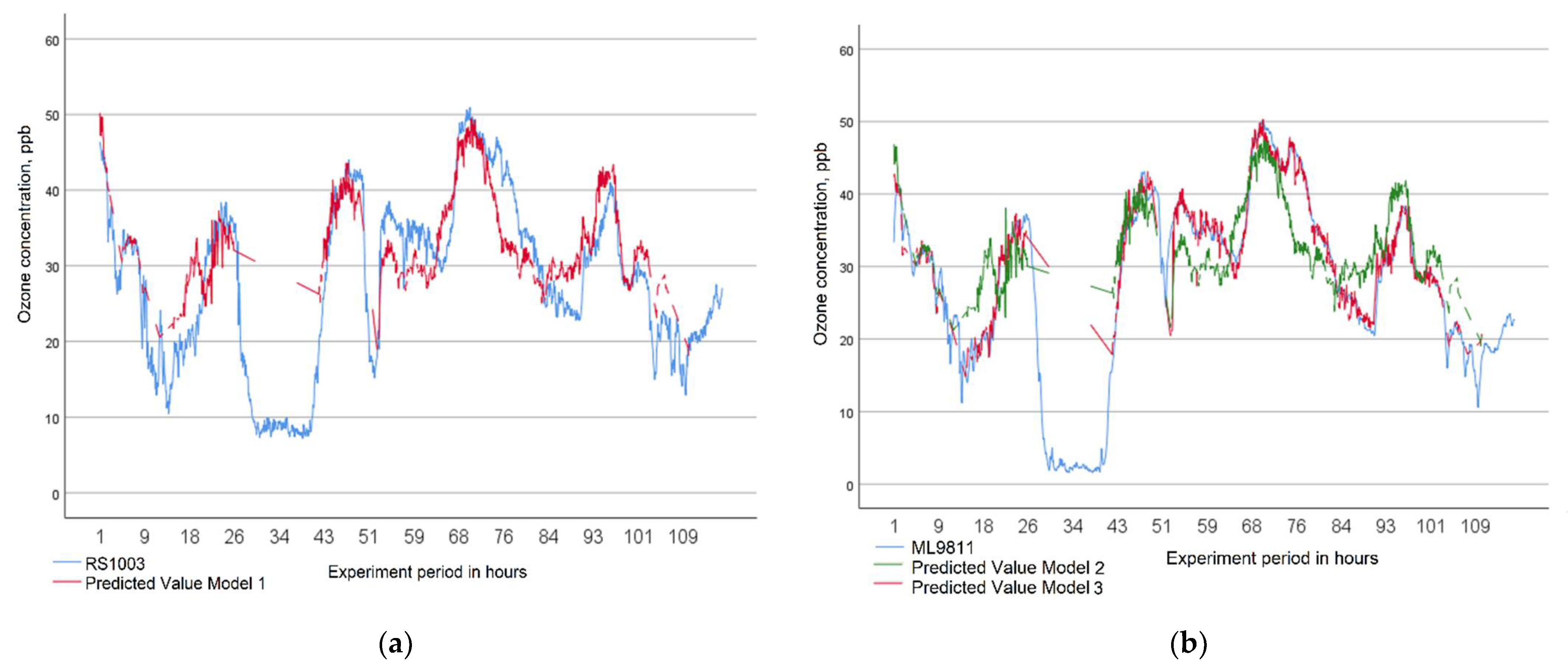
Multiple linear regression (MLR) analysis was performed to obtain the estimate of the predictive value. The following three models were designed: Model 1 was composed of the dependent variable RS and six independent variables; Model 2 had six independent variables; Model 3 has seven independent variables, all constructed to predict the ML (ozone concentration measured at a distance of 220 m). The multiple linear regression equations for the study results are presented in

Table 5. Multiple linear regression results.

1 Model	Explanation of the Model’s Equation	R2
Model 1	$RS=119.77+0.16·X_{AS}-1.71·X_{TE}-0.91·X_{HU}+0.47·X_{WS}-0.02·X_{WD}-0.005·X_{PR}$	0.635
Model 2	$ML=102.75+0.16·X_{AS}-1.30·X_{TE}-0.76·X_{HU}+0.54·X_{WS}-0.03·X_{WD}-0.003·X_{PR}$	0.493
Model 3	$ML=-33.35-0.02·X_{AS}+0.64·X_{TE}-0.28·X_{HU}+0.003·X_{WS}-0.012·X_{WD}-0.003·X_{PR}+1.14·X_{RS}$	0.944

¹ Notes: Model 1—dependent variable (RS1003 (RS)) and independent variables (aerosol particles (AS), temperature (TE), humidity (HU), wind speed (WS), wind direction (WD) and atmospheric pressure (PR)); Model 2—dependent variable (ML9811 (ML)) and independent variables (AS, TE, HU, WS, WD and PR); Model 3—dependent variable (ML) and independent variables (AS, TE, HU, WS, WD, PR and RS).

. The comparisons between the experimental and the predicted data for RS (Model 1) and for ML (Model 2 and Model 3) are shown in Figure 3. The detailed results of this study with respect to Model 1, Model 2 and Model 3 are shown in the

Table A1. Model 1 coefficients assessed by multiple linear regression for ozone concentration.

1 Model 1	Unstandardised Coefficients		Standardised Coefficients Beta	t	Sig.	Partial Eta Squared
	B	Std. Error
(Constant)	119.774	5.620		21.311	0.000	0.635
AS	0.157	0.015	0.354	10.444	0.000	0.369
TE	−1.710	0.170	−0.798	−10.085	0.000	0.123
HU	−0.910	0.047	−1.603	−19.519	0.000	0.116
WS	0.468	0.139	0.101	3.367	0.001	0.330
WD	−0.016	0.004	−0.111	−3.836	0.000	0.014
PR	−0.005	0.002	−0.085	−2.490	0.013	0.019

¹ Notes: Model 1 dependent variable (RS) and independent variables (AS, TE, HU, WS, WD and PR). Determination coefficient R Squared = 0.635 (adjusted R Squared = 0.632).

,

Table A2. Model 2 coefficients assessed by multiple linear regression for ozone concentration at a distance of 220 m.

1 Model 2	Unstandardised Coefficients		Standardised Coefficients Beta	t	Sig.	Partial Eta Squared
	B	Std. Error
(Constant)	102.752	6.772		15.174	0.000	0.229
AS	0.156	0.018	0.344	8.613	0.000	0.087
TE	−1.296	0.204	−0.591	−6.340	0.000	0.049
HU	−0.755	0.056	−1.301	−13.449	0.000	0.189
WS	0.535	0.168	0.112	3.193	0.001	0.013
WD	−0.030	0.005	−0.202	−5.945	0.000	0.044
PR	−0.003	0.002	−0.044	−1.087	0.277	0.002

¹ Notes: Model 2 dependent variable (ML) and independent variables (AS, TE, HU, WS, WD and PR). Determination coefficient R Squared = 0.493 (adjusted R Squared = 0.489).

and

Table A3. Model 3 coefficients assessed by multiple linear regression for ozone concentration at a distance of 220 m and for ozone concentration near high-voltage lines (RS).

1 Model 3	Unstandardised Coefficients		Standardised Coefficients Beta	t	Sig.	Partial Eta Squared
	B	Std. Error
(Constant)	−33.353	2.837		−11.759	0.000	0.152
AS	−0.022	0.006	−0.049	−3.483	0.001	0.015
TE	0.648	0.072	0.296	8.964	0.000	0.094
HU	0.279	0.023	0.480	12.210	0.000	0.161
WS	0.003	0.056	0.001	0.053	0.958	0.000
WD	−0.012	0.002	−0.079	−6.933	0.000	0.058
PR	0.003	0.001	0.051	3.777	0.000	0.018
RS	1.136	0.014	1.111	78.939	0.000	0.890

¹ Notes: Model 3 dependent variable (ML) and independent variables (AS, TE, HU, WS, WD, PR and RS). Determination coefficient R Squared = 0.944 (adjusted R Squared = 0.944).

of Appendix A. Valuable information about the spread of the ozone concentration levels can be enclosed by the measured models’ parameters—i.e., the standardised beta coefficients that present the contributions of each variable to the model and then t and p values that can highlight the impacts of the independent variables on the dependent variable (see Table A1 and Table A2, Appendix A).

Detailed information on the coefficients of the Model 1 parameters and their measurement accuracies is shown in Table A1. The constant achieved a large t value (t = 21.311, p < 0.000), which supports its significance. Moreover, a significant inverse correlation between RS and HU with a negative t value (t = −19.519) and a corresponding low p value (p < 0.000) was noted. Similarly, a significant inverse relationship was apparent between RS and TE (t = −10.085, p < 0.000). The t and p values confirmed the impact of the independent variables on the dependent variable. Following the measurements, all independent variables were statistically significant (p < 0.05) (see Table A1, Appendix A).

The higher significance in Model 2 appears to be the same as in the Model 1 and supports the significance of the constant (t = 15.174, p < 0.000). Additionally, a significant negative relationship between ML and HU (t = −13.449, p < 0.000) was identified. All independent variables included in this study showed significance except for PR, where p = 0.277 > 0.05. The significance of regression coefficients for Model 2 is listed in detail in Table A2 (see Appendix A).

The high t rate (t = 78.939, p < 0.000) of RS in Model 3 correspondingly supports the high significance of ML—i.e., ozone concentrations measured by ML9811 at a distance of 220 m. Moreover, a significant positive relationship between ML and HU (t = 12.210, p < 0.000) was identified. All independent variables included in this study showed significance except for WS, where p = 0.995 > 0.05. Detailed information on the coefficient values of Model 3 and their assessment is presented in Table A3 (see Appendix A); a graphical representation of the ozone concentration prediction by Model 2 is shown in Figure 3b.

Following the rule, Fisher’s F value can indicate the importance of the factors included in the model. Fisher’s F value can explain how the factors included in the model clarify the variation in the data about its mean and prove the validity of the identified effects of these factors. According to the ANOVA tests performed on the regression model, the designed models are significant, allowing the following interpretation from Fisher’s F test and significant probability values: F_Model1 = 224.406, p = 0.000 < 0.05; F_Model2 = 125.741, p = 0.000 < 0.05; F_Model3 = 1864.416, p = 0.000 < 0.05.

Additionally, the goodness of fit of the model was tested using the determination coefficient (R²), which provided a portion of how the experimental variables can explain the variability in the observed response values. In this study, the determination coefficient values of the designed models indicate the following: Model 1 (R² = 0.635) could explain 63.5% of the variability in the responses of ozone concentration near high-voltage powerlines measured by RS1003; Model 2 (R² = 0.493) can explain only 49.3% of the variability; Model 3 (R² = 0.944) can explain 94.4% of the ozone concentration levels measured by ML9811 at a distance of 220 m (see Table 5).

In addition, the adjusted coefficient of determination (adjusted R²) can also be discussed. It is a statistical value that classifies the proportion of the variation enlightened by the assessed regression line. The values of the adjusted determination coefficients for Model 1 (Adjusted R² = 0.632) and Model 3 (Adjusted R² = 0.944) are high enough to indicate a high significance of these models, except for Model 2, as R² =0.493 and adjusted R² = 0.482. The closer the adjusted R² is to 1, the better the estimated regression model (regression equation) fits or clarifies the relationship among the dependent and independent variables. Following the rule, if R² < 0.40, then the model should not be used for prediction [21].

5.3. Results of the Application of an Artificial Neural Network to Determine the Causes of Ozone Spread

The next step of this study was to develop models based on the neural network performance when predicting ozone concentration levels as measured near high-voltage powerlines (RS) and at a distance of 220 m (ML). Several ANN networks were constructed and tested, including MLP and RBF. This comprehensive analysis was completed in order to establish a satisfactory structure with an appropriate number of hidden layers and neurons, since a higher number may cause overfitting, while a smaller number may not process the data adequately. These extensive calculations were important in designing the structure of the ozone concentration prediction models in order to make them truly beneficial. These developed ANNs were trained using the learning dataset. This procedure allowed us to control the optimum quantity of neurons, hidden layers and transfer functions. The MLP and RBF models were validated according to the test dataset. Later, the best obtained network model, with the maximum coefficient of determination (R²) and minimum training and testing MSE, was preferred to predict the causes of the ozone spread.

5.3.1. Application of an ANN for Ozone Concentration Levels Near High-Voltage Powerlines

The artificial neural network was applied to determine the causes of ozone spread, as measured near high-voltage powerlines (dependent variable, RS) and at a distance of 220 m (dependent variable, ML).

The best structure with the lowest MSE was identified after repetitive model rounds using different specifications of activation functions and different proportions of training, testing and holdout layers. The carefully chosen ANN model with its specific structure offers a good representation of the prediction of the ozone spread causality.

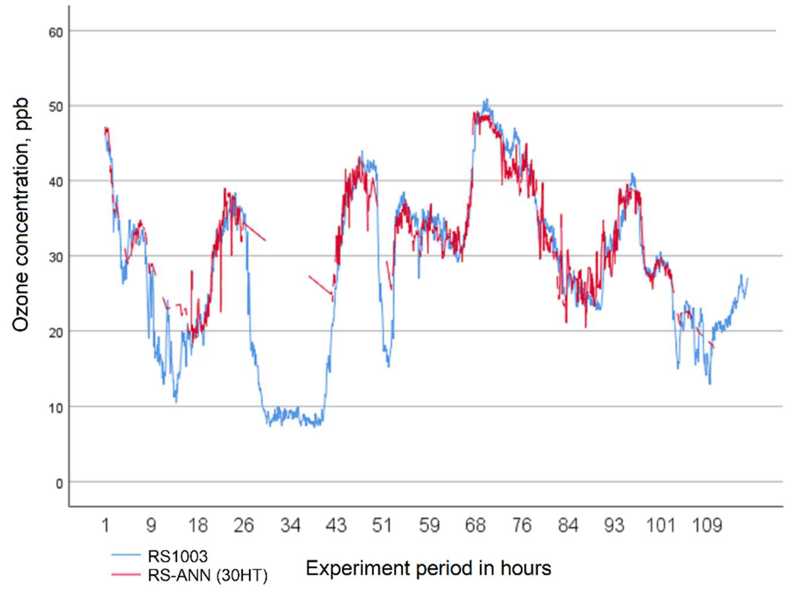
The best MLP model specification for ozone concentration levels near high-voltage powerlines (RS variable) can be described using the following parameters: first, the model’s input layer included six input variables; second, the ANN was constructed with one hidden layer and 30 neurons; third, one output layer with one output variable (RS variable). The accuracy of the model was determined to be very good because of its capacity to explain the variation of about 89% of ozone spread causality; according to the small training and testing layer errors by MSE, these were 2.665 × 10⁻³ and 2.302 × 10⁻³ for training and testing, respectively. The experimental data and the predicted data using the ANN of MLP ozone concentration spread are shown in Figure 4.

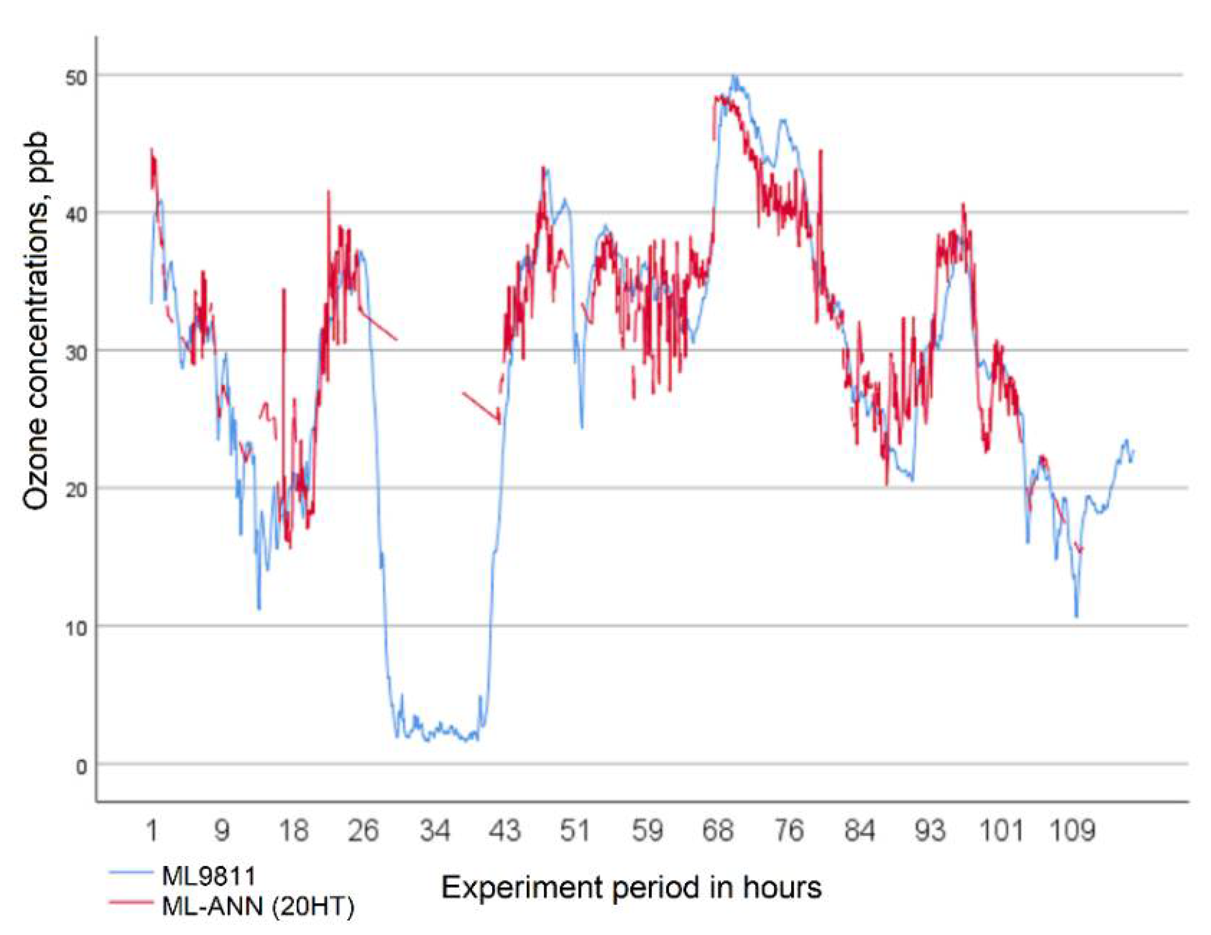
5.3.2. Application of an ANN for Ozone Concentration Levels at a Distance of 220 m

The ANN model for ozone concentrations at a distance of 220 m (dependent variable, ML) was described by six neurons (independent variables) in the input layer, where they individually corresponded to an environmental parameter; for the output layer, one neuron was used to represent the ozone concentration. The analysis of the modelling of experimental data was similar to the analysis of ozone concentrations near high-voltage power transmission lines measured by RS1003. The main focus of this continuing procedure was to determine the optimal number of hidden layer neurons.

This study background was built on the neural network training function for MLP (sigmoid and hyperbolic tangent functions) and RBF (softmax function) designs were accepted. Additionally, the number of hidden layer neurons required to obtain the most acceptable request performance was identified. In this case, the outcomes based on the mean square error measure were compared to identify the optimal model, which led us to the model we needed. After this modelling analysis, the most suitable model for predicting ozone concentration at a distance of 220 m was identified. The comparison between collected experimental data and predicted values of ozone concentrations at a distance of 220 m are shown in Figure 5.

The highest validation showed the ANN model with the specifications of: MLP network trained with six components (values were transformed by the normalised rescaling method); the 4–7–1 dataset partition of ANN layers was used with 6 neurons as inputs, 20 neurons in the hidden layer and 1 output. The outcomes of the model trained with an activation function hyperbolic tangent indicated small errors of MSE—training = 6.328 × 10⁻³ and testing = 3.785 × 10⁻³. The predicted ozone concentrations can be considered successful. Moreover, in accordance with the determination coefficient (R² = 0.80), the designed model showed good capability to explain the variation of about 80% of ozone spread causality.

5.3.3. Results of the Robustness of Established ANN Models

To test the statistical difference between two measurements, a t-test of paired models was conducted between observed and predicted data. Paired samples descriptive statistics for observed and predicted ozone concentrations are presented in

Table A4. Paired samples statistics for observed and predicted ozone concentrations.

		Mean	N	Std. Deviation	Std. Error Mean
1Pair 1	RS -RS1003	34.0560	782	7.67252	0.27437
	RS-ANN (30HT)	33.9935	782	7.03976	0.25174
2Pair 2	ML ML9811	33.6229	782	7.84919	0.28069
	ML-ANN (20HT)	33.5073	782	7.12812	0.25490

^1,2 Notes: ¹ Pair 1 ozone concentration near high-voltage lines measured by RS1003 and predicted by MLP–ANN (4–7–1 of dataset partition, activation function—hyperbolic tangent, 6 input neurons, 30 neurons in hidden layer and 1 output); ² Pair 2 ozone concentration at 220 m distance from high-voltage lines measured by ML9811 and predicted by MLP–ANN (4–7–1 of dataset partition, activation function—hyperbolic tangent, 6 input neurons, 20 neurons in hidden layer and 1 output).

, Appendix A. The conducted correlation analysis results showed that observed and predicted ozone concentrations near high-voltage lines (r = 0.95, p < 0.01) and at a 220 m distance (r = 0.90, p < 0.01) were highly and positively correlated (see

Table A5. Paired samples correlations.

		N	Correlations	Sig.
1Pair 1	RS-RS1003	782	0.946	0.000
	RS-ANN (30HT)
2Pair 2	ML ML9811	782	0.896	0.000
	ML-ANN (20HT)

^1,2 Notes: ¹ Pair 1 ozone concentration near high-voltage lines measured by RS1003 and predicted by MLP–ANN (4–7–1 of dataset partition, activation function—hyperbolic tangent, 6 input neurons, 30 neurons in hidden layer and 1 output); ² Pair 2 ozone concentration at 220 m distance from high-voltage lines measured by ML9811 and predicted by MLP–ANN (4–7–1 of dataset partition, activation function—hyperbolic tangent, 6 input neurons, 20 neurons in hidden layer and 1 output).

, Appendix A). Moreover, the t-test identified an insignificant average difference between ozone concentrations observed by the RS1003 sensor and those predicted by MLP–ANN (30HT) (t₇₈₁ = −0.697, p = 0.486). The detailed information is presented in

Table 8. Details of design paired samples t-test to assess differences.

Pair	Paired Differences					3 Student’s t-Test
	Mean	Std. Deviation	Std. Error Mean	95% CI of the Difference
				Lower	Upper	t	df	p
1 Pair 1	0.063	2.507	0.090	−0.114	0.239	0.697	781	0.486
2 Pair 2	0.116	3.483	0.125	−0.129	0.360	0.928	781	0.354

^1,2 Notes: ¹ Pair 1 ozone concentration near high-voltage lines measured by RS1003 and predicted by MLP–ANN (4–7–1 of dataset partition, activation function—hyperbolic tangent, 6 input neurons, 30 neurons in hidden layer and 1 output); ² Pair 2 ozone concentration in account of 220 m distance from the high-voltage lines measured by ML9811 and predicted by MLP–ANN (4–7–1 of dataset partition, activation function—hyperbolic tangent, 6 input neurons, 20 neurons in hidden layer and 1 output). ³ Student’s t-test, df = degrees of freedom and p = Sig. (2-tailed).

.

Subsequently, the observed ozone concentrations at a distance of 220 m by the ML9811 sensor and predicted ozone concentrations by MLP–ANN (20HT) (t₇₈₁ = −0.928, p = 0.354) were evaluated. According to the average of observed and predicted ozone concentrations, it was identified that the observed ozone concentrations were equivalent to a 95% confidence interval, CI $\in$ [−0.114, 0.239]. Furthermore, observed ozone concentrations at a distance of 220 m were similar to those predicted by 95% confidence intervals, CI $\in$ [−0.129, 0.360]. The results of the conducted tests established the strength of the designed ANN models with no significant difference between experimentally observed and predicted data.

6. Discussion

The experiment was carried out near a village (55°34′ N, 25°38′ E) in the eastern part of Lithuania in September 2019. The field investigations were carried out near two high-voltage power transmission lines of 330 kV and at a distance of 220 m from the powerlines (see Figure 2b). A total of 1388 measurements were collected, but the survey analysis used 782 measurements of full and complete data only. The dataset was reduced before modelling, taking into account that wind speed was close to 0 m/s for almost 40% of the experiment time, which made it impossible to assess wind direction.

Descriptive analysis and forecasting models designed to assess/measure ozone concentration were performed and utilized. Firstly, SPSS 26v was used to assess the correlations between the meteorological parameters and air pollution using Pearson’s correlation coefficients. Additionally, the multiple regression models, MLP and RBF neural network structures were employed in this study to make accurate predictions about the influence of meteorological conditions and high-voltage powerlines on ground-level ozone formation. This type of analysis was in line with other similar surveys [12,13,14,15,16].

A multiple regression analysis was carried out to determine the environmental factors manipulating ozone concentration and to assess them in the order of effect importance. The Partial Eta Squared (PES) test identified that the most important meteorological factors influencing the variations in ozone levels for Model 1, Model 2 and Model 3 are the following: temperature (TE), wind speed (WS), atmospheric pressure (PR) and relative humidity (HU). These findings are in line with the investigation results presented by Dueñas et al. [20] and other scholars [22]. In addition, the results of this study identified that the order of the effect of meteorological factors on predicting ozone concentrations differs significantly. The results appear to be influenced by measuring distance; the importance of factors near high-voltage powerlines (Model 1, Table A1 in Appendix A) is as follows: AS > WS > TE > HU > PR > WD; at a distance of 220 m, the influential factors are ranked in a slightly different order, as follows: HU > AS > TE > WD > WS > PR (Model 2, Table A2 in Appendix A). Model 3 was supplemented with the independent variable describing the ozone concentration amounts near high-voltage lines and was identified by RS1003 (variable RS, Model 3, Table A3 in Appendix A). The calculation results showed that the parameters of Model 3 were mutually affected in a different way compared to Model 2. According to the PES test, the order of factors by importance is as follows: RS > HU > TE > WD > PR > AS. These parameters are significant enough to forecast ozone concentrations. Moreover, in Model 3, the variable WS was identified as insignificant (t = 0.053, p = 0.958, see Table A3 in Appendix A) and had to be eliminated in future analysis. The principal effects of the variables on ozone concentration are presented in Table A1, Table A2 and Table A3 (Appendix A).

A number of ANN models were surveyed to predict and model air pollution by way of ozone concentration levels. In order to construct the optimal models, the experimental data of the environmental conditions with significant correlations were used. In fact, the higher significance and the most influential value for ozone concentration forecasting in the results of the conducted study on ANNs models showed only a few control parameters. The most significant environmental parameters identified in the designed ANN models were those that were highly related to dependent variables by calculated correlation coefficients [35].

Moreover, the statistical analyses conducted on the data showed that the determination coefficient R², which is an indicator of the goodness of fit of the designed model, was close to 96%. Accordingly, it can be determined that less than 14% of the overall variations were not explained by the model, which in turn demonstrates a highly accurate estimation. R² defines the amount of the variance by evaluating the data explained by the model. R² ranges from 0 to 1, with higher values identifying lower error variance, where measures over to 0.5 are considered appropriate [20].

Our findings highlight the potent capacity of ANNs to model and predict parameters in complex natural environments, such as forecasting air pollution [35], which is consistent with earlier research. Accordingly, this tool could replace the deterministic models of prediction that have demonstrated their incompetence in complex environments. In conclusion, ANNs could be used as primary warning systems before the pollution occurs in order to avoid or mitigate the negative effects of air contamination.

7. Conclusions

In this study, artificial intelligence approaches were used to model and predict the concentrations of ozone as an air pollutant by using experimental data. The complex experimental and theoretical research on the formation and distribution of pollutants in the environment of anthropogenic sources of pollution has revealed the peculiarities of distribution and correlation of important researched pollutants with meteorological parameters and highlighted the role of high-voltage power transmission lines in ozone formation.

According to the survey results, the ANN–MLP method was more accurate compared to the ANN–RBF method and the MLR method in modelling and predicting the ozone concentration levels with respect to the meteorological parameters. The MLP model with an activation hyperbolic tangent function with six inputs, twenty neurons in one hidden layer and a determination coefficient higher than 90% was identified as the most suitable one for ozone concentration prediction measured near high-voltage powerlines. Furthermore, a different model was optimised for ozone concentration prediction measured at a distance of 220 m, with an activation sigmoid function with six inputs, twenty-five neurons in one hidden layer and a determination coefficient higher than 90%.

Therefore, it could be concluded that the selected parameters were appropriate for the development and use of the network structures, as well as for the selection of the input variables based on the correlations between the variables, with the air pollutants reducing the number of the input variables and producing acceptable results.

This study proposes a method to simultaneously analyse multiple factors. A statistical experimental design was used to enhance ozone production by high-voltage powerlines and its spread at a distance of 220 m. The findings suggest that the different components show a significant influence on the increase in ozone concentration levels. In Model 3, temperature and humidity played the most significant role, whereas, in Models 1 and 2, the aerosol particles and wind speed were the factors that increased the ozone concentration levels. Furthermore, high temperature and humidity decreased the ozone concentration levels in Model 2.

Remarkably, the calculated results in this survey demonstrated that ANN predictions are possibly more effective than MLR predictions. Additionally, the designed artificial neural network provided a perfect level of correct predictions for responses than the multiple linear regression methods. Therefore, ANN analysis appears to be a more effective method of predicting ozone concentrations. This result specifies that the forecast of ozone concentration levels may encompass a complex nonlinear relationship.

Moreover, the investigation results proved that MLP seems to be the most adequate ANN model for forecasting ozone concentrations. However, the activation function and the number of neurons in the hidden layer is specific to each type of prediction (ozone concentrations near high-voltage lines and at a distance of 220 m).

Initially, the aims of the current survey were to determine an adequate topology of ANNs and multiple linear regression models for forecast of ozone concentrations near high-voltage lines and at a distance of 220 m. Secondly, this study aimed to select the best method for predicting ozone as an air pollutant and in turn select an improved topology.

The conducted calculations led to the identification of the capability of ANNs to recognise complex structures in datasets which otherwise may not be explained as well by a simple mathematical model. Actually, this research confirmed that computational tools such as ANNs can be effectively used to clarify these types of problems.

A further problem is that the number of optimised errors the RBFN models acquired with the activation function softmax algorithm is too big (this was identified only in assessment with the models of MLP neural networks which used the hyperbolic tangent and sigmoid as activation functions). According to this, future work should address this limitation and extend the analysis.

References

- Hamza, A.-S.H. Evaluation and measurement of magnetic field exposure over human body near EVL transmission lines. Electr. Power Syst. Res. 2005, 74, 105–118. [Google Scholar] [CrossRef]
- Ogan, V.N.; Bendor, S.A.; James, A.E. Analysis of Corona Effect on Transmission Line. Am. J. Eng. Res. (AJER) 2017, 6, 75–87. [Google Scholar]
- Еланский, Н.Ф.; Невраев, А.Н. Высоковольтные линии электропередач как возможный источник озона в атмосфере. Доклады Академии Наyк (ДАН) 1999, 365, 533–536. [Google Scholar]
- Elansky, N.F.; Panin, L.V.; Belikov, I.B. Influence of High-Voltage Lines on the Surface Ozone Concentration. Atmos. Ocean. Phys. 2001, 37, S10–S23. [Google Scholar]
- Brown, P. New Evidence Power Lines Cause Cancer. 2007. Available online: http://www.rense.com/general3/pwoerlines.htm (accessed on 1 September 2020).
- Yahaya, E.A.; Jacob, T.; Nwohu, M.; Abubakar, A. Power loss due to Corona on High Voltage Transmission Lines. IOSR J. Electr. Electron. Eng. 2013, 8, 14–19. [Google Scholar] [CrossRef]
- Li, C.Y.; Sung, F.P.-C.; Chen, F.-L.; Lee, P.-C.; Silva, M.; Mezei, G. Extremely-low-frequency magnetic field exposure of children at schools near high voltage transmissions lines. Sci. Total Environ. 2007, 376, 151–159. [Google Scholar] [CrossRef] [PubMed]
- Jung, J.-S.; Lee, J.W.; Arachchige Don, R.K.M.; Park, D.S.; Hong, S.C. Characteristics and potential human health hazards of charged aerosols generated by high-voltage power lines. Int. J. Occup. Saf. Ergon. 2019, 25, 91–98. [Google Scholar] [CrossRef] [PubMed]
- Ivancsits, S.; Diem, E.; Jahn, O.; Rudiger, H.W. Intermittent extremely low frequency electromagnetic fields cause DNA damage in a dose-dependent way. Int. Arch. Occup. Environ. Health 2003, 76, 431–436. [Google Scholar] [CrossRef]
- Draper, G.; Vincent, T.; Kroll, M.E.; Swanson, J. Childhood cancer in relation to distance from high voltage power lines in England and Wales: A case-control study. Br. Med. J. 2005, 330, 1–5. [Google Scholar] [CrossRef] [PubMed] [Green Version]
- Djalel, D.; Mourad, M. Study of the influence high-voltage power lines on environment and human health (case study: The electromagnetic pollution in Tebessa city, Algeria). J. Electr. Electron. Eng. 2014, 2, 1–8. [Google Scholar] [CrossRef]
- Bai, Y.; Li, Y.; Wang, X.; Xie, J.; Li, C. Air pollutants concentrations forecasting using back propagation neural network based on wavelet decomposition with meteorological conditions. Atmos. Pollut. Res. 2016, 7, 557–566. [Google Scholar] [CrossRef]
- Cheng, W.; Shen, Y.; Zhu, Y.; Huang, L. A Neural Attention Model for Urban Air Quality Inference: Learning the Weights of Monitoring Stations. Available online: https://www.aaai.org/ocs/index.php/AAAI/AAAI18/paper/download/16607/15925 (accessed on 1 September 2020).
- Gantt, B.; Meskhidze, N.; Zhang, Y.; Xu, J. The effect of marine isoprene emissions on secondary organic aerosol and ozone formation in the coastal United States. Atmos. Environ. 2010, 44, 115–121. [Google Scholar] [CrossRef]
- Wang, J.; Wang, Y.; Liu, H.; Yang, Y.; Zhang, X.; Li, Y.; Zhang, Y.; Deng, G. Diagnostic identification of the impact of meteorological conditions on PM2.5 concentrations in Beijing. Atmos. Environ. 2013, 81, 158–165. [Google Scholar] [CrossRef]
- Wu, Q.; Xu, W.; Shi, A.; Li, Y.; Zhao, X.; Wang, Z.; Li, J.; Wang, L. Air quality forecast of PM10 in Beijing with Community Multi-scale Air Quality Modeling (CMAQ) system: Emission and improvement. Geosci. Model. Dev. 2014, 7, 2243–2259. [Google Scholar] [CrossRef] [Green Version]
- Feng, Y.; Zhang, W.; Sun, D.; Zhang, L. Ozone concentration forecast method based on genetic algorithm optimized back propagation neural networks and support vector machine data classification. Atmos. Environ. 2011, 45, 1979–1985. [Google Scholar] [CrossRef]
- Ozel, G.; Cakmakyapan, S. A new approach to the prediction of PM10 concentrations in Central Anatolia Region, Turkey. Atmos. Pollut. Res. 2015, 6, 735–741. [Google Scholar] [CrossRef]
- Saide, P.E.; Carmichael, G.R.; Spak, S.N.; Gallardo, L.; Osses, A.E.; Mena-Carrasco, M.A.; Pagowski, M. Forecasting urban PM10 and PM2.5 pollution episodes in very stable nocturnal conditions and complex terrain using WRF–Chem CO tracer model. Atmos. Environ. 2011, 45, 2769–2780. [Google Scholar] [CrossRef]
- Dueñas, C.; Fernandez, M.C.; Caňete, S.; Carretero, J.; Liger, E. Assesment of ozone variations and meteorological effects in an urban area in the Mediterranean coast. Sci. Total Environ. 2002, 299, 97–113. [Google Scholar] [CrossRef]
- Gao, M.; Yin, L.; Ning, J. Artificial neural network model for ozone concentration estimation and Monte Carlo analysis. Atmos. Environ. 2018, 184, 129–139. [Google Scholar] [CrossRef]
- Paschalidou, A.K.; Karakitsios, S.; Kleanthous, S.; Kassomenos, P.A. Forecasting hourly PM10 concentration in Cyprus through artificial neural networks and multiple regression models: Implications to local environmental management. Environ. Sci. Pollut. Res. 2011, 18, 316–327. [Google Scholar] [CrossRef]
- Bekesiene, S.; Hoskova-Mayerova, S. Automatic Model Building for Binary Logistic Regression by Using SPSS 20 Software. In Proceedings of the 18th Conference on Applied Mathematics (APLIMAT 2019), Bratislava, Czech Republic, 5–7 February 2019; pp. 31–40. [Google Scholar]
- Hoskova-Mayerova, S.; Talhofer, V.; Otrisal, P.; Rybansky, M. Influence of weights of geographical factors on the results of multicriteria analysis in solving spatial analyses. ISPRS Int. J. Geo-Inf. 2020, 9, 489. [Google Scholar] [CrossRef]
- Miller, J.N.; Miller, J.C. Statistics and Chemometrics for Analytical Chemistry; Prentice Hall: London, UK, 2000. [Google Scholar]
- Pachepsky, Y.A.; Timlin, D.; Varallyay, G. Artificial neural networks to estimate soil water retention from easily measurable data. Soil Sci. Soc. Am. J. 1996, 60, 727–733. [Google Scholar] [CrossRef]
- Malinova, T.; Guo, Z.X. Artificial neural network modelling of hydrogen storage properties of Mg-based alloys. Mater. Sci. Eng. A 2004, 365, 219–227. [Google Scholar] [CrossRef]
- Song, R.G.; Zhang, Q.Z.; Tseng, M.K.; Zhang, B.J. The application of artificial neural networks to the investigation of aging dynamics in 7175 aluminium alloys. Mater. Sci. Eng. C. 1995, 3, 39–41. [Google Scholar] [CrossRef]
- Wu, S.; Feng, Q.; Du, Y.; Li, X. Artificial neural network models for daily PM10 air pollution index prediction in the urban area of Wuhan, China. Environ. Eng. Sci. 2011, 28, 357–363. [Google Scholar] [CrossRef]
- Hochreiter, S.; Schmidhuber, J. Feature extraction through LOCOCODE. Neural Comput. 1999, 11, 679–714. [Google Scholar] [CrossRef] [PubMed]
- Neruda, R.; Kudova, P. Learning methods for radial basis function networks. Future Gener. Comput. Syst. 2005, 21, 1131–1142. [Google Scholar] [CrossRef]
- Van Liew, M.W.; Arnold, J.G.; Garbrecht, J.D. Hydrologic simulation on agricultural watersheds: Choosing between two models. Trans. ASAE 2003, 46, 1539–1551. [Google Scholar] [CrossRef]
- Sykora, P.; Kamencay, P.; Hudec, R.; Benco, M.; Sinko, M. Comparison of Neural Networks with Feature Extraction Methods for Depth Map Classification. Adv. Mil. Technol. 2020, 15, 1. [Google Scholar] [CrossRef]
- Yang, Y.-K.; Sun, T.-Y.; Huo, C.-L.; Yu, Y.-H.; Liu, C.-C.; Tsai, C.-H. A novel self-constructing Radial Basis Function Neural Fuzzy System. Appl. Soft Comput. J. 2013, 13, 2390–2404. [Google Scholar] [CrossRef]
- Domańska, D.; Wojtylak, M. Application of fuzzy time series models for forecasting pollution concentrations. Expert Syst. Appl. 2012, 39, 7673–7679. [Google Scholar] [CrossRef]