Analysis of a k-Stage Bulk Service Queuing System with Accessible Batches for Service

Abstract

In most of the service systems considered so far in queuing theory, no fresh customer is admitted to a batch undergoing service when the number in the batch is less than a threshold. However, a few researchers considered the case of customers accessing ongoing service batch, irrespective of how long service was provided to that batch. A queuing system with a different kind of accessibility that relates to a real situation is studied in the paper. Consider a single server queuing system in which the service process comprises of k stages. Customers can enter the system for service from a node at the beginning of any of these stages (provided the pre-determined maximum service batch size is not reached) but cannot leave the system after completion of service in any of the intermediate stages. The customer arrivals to the first node occur according to a Markovian Arrival Process $\left(MAP\right)$. An infinite waiting room is provided at this node. At all other nodes, with finite waiting rooms (waiting capacity $c_j,2\le j\le k$), customer arrivals occur according to distinct Poisson processes with rates ${\lambda }_j,2\le j\le k$. The service is provided according to a general bulk service rule, i.e., the service process is initiated only if at least a customers are present in the queue at node 1 and the maximum service batch size is b. Customers can join for service from any of the subsequent nodes, provided the number undergoing service is less than b. The service time distribution in each phase is exponential with service rate ${\mu }_j^m$, which depends on the service stage $j,1\le j\le k$, and the size of the batch $m,a\le m\le b$. The behavior of the system in steady-state is analyzed and some important system characteristics are derived. A numerical example is presented to illustrate the applicability of the results obtained.

1. Introduction

A detailed literature survey of bulk service queueing systems can be found in [1,2]. In most of the works, customer service is provided in batches of varying sizes with minimum batch size a and maximum batch size b-also called general bulk service (GBS) rule (introduced by Neuts [3]). In that paper, the author assumes that a minimum of a customers are required to start a service. This is referred to as the quorum. The maximum permissible batch size is set as $b(a<b)$. Therefore, at a service completion epoch, if more than b customers are in the queue, the server takes the first b among those waiting for service and the remaining customers have to wait until their turn comes. If the number of customers waiting when the service of the current batch is completed is between a and b, both included, then all of them are taken together for service. On the other hand, if only less than a customers are waiting in the queue at the epoch of service completion, then the server stays idle or goes on a vacation. The motivation for this assumption is economic—that offering service with at least a customers in each service batch reduces cost. Airport shuttles follow this rule. There are several other examples in real life that fit into this definition. In literature, certain batch service queuing systems are considered wherein customers can join or access an ongoing service batch any time before service of the batch is completed, provided the specified maximum service batch size is not reached. The assumption made in that admission strategy is that customers who join during an ongoing service batch will not increase the total service time of the batch. Queuing systems with accessible batch service have been studied quite extensively and many variants of the same can be found in the literature. A brief survey of literature on queuing systems with accessible batches can be found in the next paragraph.

Continuous-time queuing systems with accessible service batches have been studied in the literature (see [4,5,6,7,8,9,10,11,12]), while discrete-time queues with accessible and non-accessible batches are considered in [13,14,15,16,17,18,19,20]. The steady-state and transient distribution of system states for a single server queuing system with Poisson arrivals and exponential service to a single customer or to a batch (depending on the number of customers in the queuing system) are studied in [6,8], respectively. If the number of customers in the system is less than c, service will be provided singly. Otherwise, service is provided in batches. Late arrivals can access the system until the number in a batch is less than d, but greater than or equal to c. As an extension to the above models, bulk service queuing systems with service according to a Modified General Bulk Service Rule (Server starts service only when queue size is at least c. The server continues to serve at a service completion epoch even when the number in queue is less than c but greater than or equal to $a\le c$) in addition to assumptions in previous models ([6,8]) are analyzed in [10] (Continuous case) and [20] (Discrete case). Krishnamoorthy and Ushakumari analyze a finite as well as infinite capacity single server queuing system with Poisson arrivals and exponential service (with service rate depending on the number of customers in the system) in [7]. In this paper, it is assumed that, though customers depart individually from the system, service is provided either singly or accessible batches. In [11,12], a finite (infinite buffer) bulk queuing system with renewal input and exponential service provided either singly or in batches, depending on the number of customers present in the system, is studied (the difference being that, in [12], accessibility to an ongoing service is restricted to a threshold value d). In [5], Ayappan and Renganathan consider a single server preemptive priority queue in which high priority customers are given service in batches according to GBS Rule and with accessibility to batches, while low priority customers are provided service singly. Bulk service queues with accessible and/or non- accessible batches (finite and/or infinite buffer queues) having geometrically distributed inter-arrival as well as service times are analyzed in [13,14,15]. A discrete-time bulk service queue with geometrically distributed inter-arrival times, accessibility to service batches, and service times following negative binomial distribution is studied in [16]. Bulk service vacation queueing systems with accessible batches have been studied in [19,21,22,23,24]. Additionally, in [23], the service batch sizes are assumed to be Markov dependent. A two-server queueing system in which server 1 alone provides accessible batch service is analyzed in [25]. Though permitting customers to join an ongoing service batch helps in reducing congestion and waiting time in queues, it is not often very realistic. A customer who wishes to get service from the very beginning may be forced to join an ongoing service batch. On the contrary, some customers might not require an entire service but just a part of it, and, for them, joining the service from the very beginning will increase their waiting time or results in a higher cost for service (to be paid by such customers).

The queuing system considered in the present paper overcomes these shortcomings as service is assumed to be provided in stages, and customers can access an ongoing service batch from the beginning of these stages, depending on their requirement. This queuing model is immediately seen to be applied in elevators and transport systems. More specifically, consider an organization (could be an office/educational institution/an exhibition, etc.), where people go to get some work done. A public transport system operates to ferry people to this destination from different locations in the city. Individuals seeking service of the organization queue up at different locations (Henceforth, these specific locations will be referred to as nodes). Node 1 is the starting point where an infinite capacity waiting space is provided. At all other nodes, only finite capacity waiting rooms are provided. The transport system collects passengers from different nodes numbered $1,2,\dots k$ in that order. Finally, it reaches the destination. The transport vessel has only finite capacity b, and it starts service from node 1 the moment a minimum of a passengers are available. However, more people can board the transport, subject to the capacity restriction. In case it starts with b passengers from node 1, then no more passengers can board it from that node or from any intermediate nodes. If the transport starts from node 1 with less than b passengers then, from intermediate nodes, the resulting number of passengers who could board the transport is such that the number of passengers in the system does not exceed b. One can as well study the case of passengers returning from the organization; in this case, the effect will be reversed because passengers alight at different intermediate nodes: $k,k-1,\dots$ and finally at 1, if there is any. This will be taken up in a future study.

The model being discussed in this paper could also be applied to inventory transport. Raw materials are collected from different locations to be transported to a manufacturing plant. The raw material available at node 1 is the maximum needed item. The remaining items to be collected at nodes 2 through k are used as catalysts and so their consumption is minimum. Thus, at node 1, maximum quantity is collected, subject to capacity restriction; only if this capacity restriction is not reached will commodities at remaining nodes be collected. Furthermore, we can impose storage capacity restrictions at the plant. Based on this, the optimal transportation schedule is to be drawn. The availability of materials at the various nodes is also to be taken into consideration. This will be a direction for future investigation.

Another example is the lateral entry system followed in academic institutions. In Engineering Bachelor’s degree program (4 years = 8 semesters), freshers are admitted to semester 1. Those who already have a Diploma (a 3-year program) can opt to join when the other batch reaches the 3rd semester. There are several other examples from real life for the model discussed in this paper. The highlights of the present paper are:

• It introduces the concept of customer accessing an ongoing service at the start of any service stage from where it requires service rather than accessing service of an ongoing batch, upon the customer’s arrival.
• There are numerous papers in bulk service queuing literature in which service time depends on the size of a service batch. In this paper, we go further to assume that service rate depends on both the stage of service and number of customers undergoing service in the current stage.

However, we should admit that the model discussed can be further extended to cover much more general arrival and service pattern—for example, marked Markovian arrival processes $\left(MMAP\right)$ or even batch Markovian arrival processes $\left(BMAP\right)$ (batch arrivals) and phase-type service. However, the phase-type service is not appropriate because, in transport systems, there are rarely backward stage transitions. In the following sentences, the restriction of the model analyzed is summarized. The arrival process to the first node is a fairly general process, namely Markovian arrival process $\left(MAP\right)$; for arrivals to the remaining nodes, we could have also made this assumption; however, it results in a tremendous increase in the dimension of the process under consideration. Even with a Marked Markovian arrival process $\left(MMAP\right)$ assumption for arrivals to all nodes, there is a dimensionality problem.

2. The Model

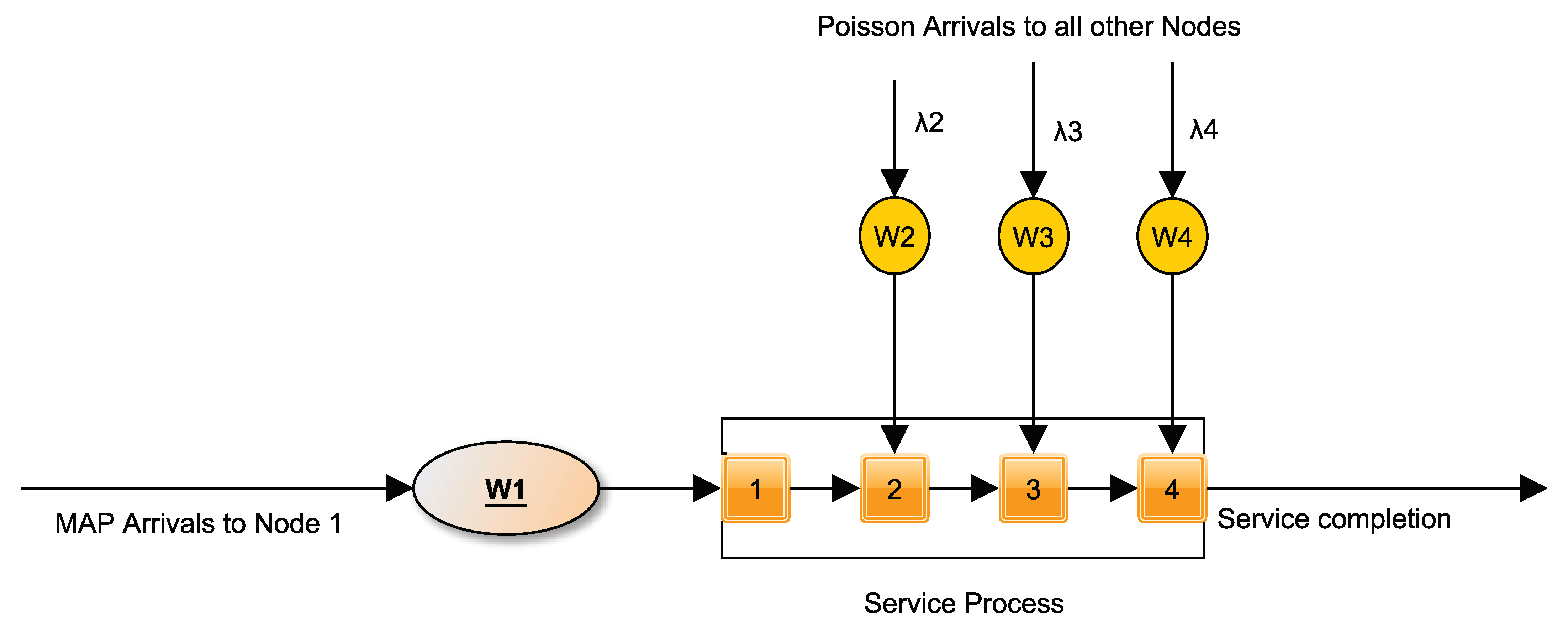
We consider a single server queuing system where the server provides service in k stages. Service is in batches. At node 1, there should be no less than a customers to start the service; but at most b can get into service. At node 2, new customers, waiting at node 2, can join this batch when it completes the first stage of service, provided the size of the batch is less than b. The number of customers joining the service batch at this node is equal to $min\{d_2,b-b_1\}$, where $b_1$ is the number of customers in the batch in stage 1 and $d_2$ is the number waiting at node 2. In general, at node j, $min\{d_j,b-b_{j-1}\}$ customers join for service in the batch when it completes service in stage $j-1$. Customers requiring service right from stage 1 (who arrive while service is progressing in stage 1 or beyond), queue up before node 1 in an infinite capacity waiting room. Only those customers requiring service from stages starting from $2/3/\dots k$ alone are to wait in the respective nodes; each of these nodes is provided finite waiting rooms (i.e., waiting room capacity $c_j$ is assumed to be finite for nodes through 2 to k). The reason for not considering the case of infinite capacity intermediate nodes is that it is impossible to analyze it with the technique adopted at present. This will be considered in a follow-up paper. Though customers can access service from intermediate nodes, they cannot leave the system after completing service from an intermediate node. Customer arrivals to node 1 follow $MAP$ with representation $(D_0,D_1)$. The entries of matrices $D_0$ and $D_1$ denote, respectively, the transition rates of the underlying $CTMC$ on r phases with and without arrivals. The expected number of arrivals per unit of time in stationary mode or the fundamental rate of $MAP$ is defined as ${\lambda }_1=\mathit{\theta }{D}_1\mathbf{e}$, $\mathit{\theta }$ is the stationary probability vector of the underlying $CTMC$ of $MAP$ (i.e., $\mathit{\theta }$ satisfies $\mathit{\theta }D=0,\mathit{\theta }\mathit{e}=1,D=D_0+D_1$). The input flow to nodes $2,3\dots k$ follow Poisson process with respective arrival rates ${\lambda }_j$. The service time at stage j is exponentially distributed with parameter ${\mu }_j^m$ which depends on the stage j; $1\le j\le k$ and the size of the service batch at that stage m; $a\le m\le b$. The pictorial representation of a queueing system in which service is provided in four phases is as shown in Figure 1.

The above queueing model can be studied as a $CTMC$ as described below. First, we introduce some notations:

• $N_j\left(t\right)$-number of customers in the queue at node j at time t
• $S\left(t\right)$-size of the batch undergoing service, if any, at time t
• $J\left(t\right)$-the stage of the service process if any, at time t
• $I\left(t\right)$-the underlying phase of $MAP$ at node 1

Then, $\{(N_1\left(t\right),N_2\left(t\right),\dots N_k\left(t\right),S\left(t\right),J\left(t\right),I\left(t\right)):t\ge 0\}$ is a $CTMC$ on state space $\Omega ={\Omega }_1\cup {\Omega }_2$ where, ${\Omega }_1=\{(n_1,n_2,\dots ,n_k,i):0\le n_1\le a-1;0\le n_2\le c_2;\dots 0\le n_k\le c_k;1\le i\le r\}$ and ${\Omega }_2=\{(n_1,n_2,\dots ,n_k,m,j,i):n_1\ge 0;0\le n_2\le c_2;\dots 0\le n_k\le c_k;a\le m\le b;1\le j\le k;1\le i\le r\}.$ ${\Omega }_1$ denotes the set of states whence the server is idle and ${\Omega }_2$ denotes the set of states whence the server is serving a batch of size m in stage j. The states are arranged in lexicographic order.

The infinitesimal generator matrix is

$${\mathcal{Q}}_1=\left[\begin{array}{cccccccccccccccc}{B}_{00}& B_{01}& & & & & & & & & & & & & & \\ & B_{11}& B_{12}& & & & & & & & & & & & & \\ ⋮& & \ddots & \ddots & & & & & & & & & & & & \\ B_{a-1a}& & & B_{a-1a-1}& B_{a-1a}& & & & & & & & & & & \\ B_{a0}& & & & B_1& B_0& & & & & & & & & & \\ B_{a+10}& & & & & B_1& B_0& & & & & & & & & \\ ⋮& & & & & & \ddots & \ddots & & & & & & & & \\ B_{b0}& & & & & & & B_1& B_0& & & & & & & \\ & B_{b+11}& & & & & & & B_1& B_0& & & & & & \\ & & \ddots & & & & & & & \ddots & \ddots & & & & & \\ & & & B_{b+aa-1}& & & & & & & B_1& B_0& & & & \\ & & & & B_2& & & & & & & B_1& B_0& & & \\ & & & & & B_2& & & & & & & B_1& B_0& & \\ & & & & & & \ddots & & & & & & & \ddots & \ddots & \end{array}\right]$$

Here, $B_{l{l}^{\prime }}$ denotes the transition rate matrix from $n_1=l$ to $n_1=l^{\prime }$. $B_0=I\otimes D_1$ denotes the transition rate matrix from $n_1$ to $n_1+1;n_1\ge a$, $B_1$ denotes the transition rate matrix within level $n_1;n_1\ge a$ and $B_2=I\otimes \left[\begin{array}{cccc}0& 0& \dots & E_{k1}\otimes {\mu }_k^a{I}_r\\ 0& 0& \dots & E_{k1}\otimes {\mu }_k^{a+1}{I}_r\\ ⋮& & ⋮\\ 0& 0& \dots & E_{k1}\otimes {\mu }_k^b{I}_r\end{array}\right],E_{k1}={\mathbf{e}}_k\left(k\right).{\mathbf{e}}_1^{\prime }\left(k\right)$ transition rate matrix from $n_1$ to $n_1-b,n_1\ge a+b$. The order of $B_0,B_1,B_2$ being $(c_2+1)\dots (c_3+1)\dots (c_k+1)\dots (b-a+1).k.r.$

As an illustration, the infinitesimal generator matrix when $a=2$ and $b=4$ is

$${\mathcal{Q}}_1=\left[\begin{array}{cccccccccc}{B}_{00}& B_{01}& & & & & & & & \\ B_{10}& B_{11}& B_{12}& & & & & & & \\ B_{20}& 0& B_1& B_0& & & & & & \\ B_{30}& 0& 0& B_1& B_0& & & & & \\ B_{40}& 0& 0& 0& B_1& B_0& & & & \\ 0& B_{51}& 0& 0& 0& B_1& B_0& & & \\ 0& 0& B_2& 0& 0& 0& B_1& B_0& & \\ 0& 0& 0& B_2& 0& 0& 0& B_1& B_0& \\ & & & & \ddots & & & & \ddots & \ddots & & & \end{array}\right]$$

If the service begins with none or a single customer, the matrix $Q_1$ will be of $GI/M/1$ type. Otherwise, this can be brought to the $GI/M/1$ type queue by redefining the level using a. Redefine level $0,l\left(0\right),$ to include states with $n_1=0,1,\dots a-1$, level $1,l\left(1\right),$ to include states with $n_1=a,a+1,\dots 2a-1$ and, in general level $n,l\left(n\right),$ to include states with $n_1=na,na+1\dots (n+1)a-1.$ Then, infinitesimal matrix changes to

$${\mathcal{Q}}_2=\left[\begin{array}{cccccccccc}{C}_{00}& C_{01}& & & & & & & & \\ C_{10}& C_1& C_0& & & & & & & \\ C_{20}& C_2& C_1& C_0& & & & & & \\ C_{30}& C_3& C_2& C_1& C_0& & & & & \\ C_{40}& C_4& C_3& C_2& C_1& C_0& & & & \\ & & & \ddots & & \ddots & \ddots & & & \end{array}\right]$$

$C_0={\mathbf{e}}_a\left(a\right)\times {\mathbf{e}}_1^{\prime }\left(a\right)\otimes B_0$.

Let $s=\frac{a+b}{a}$, if it is an integer and $s=\left[\frac{a+b}{a}\right]+1$, otherwise.

$C_i=\mathbf{0};i>s$ and $C_{i0}=\mathbf{0};i\ge s$.

(The reason being that $sa-b$ belongs to level 1 and hence there is no transition from level s to level 0.)

For the example considered above,

$$C_{00}=\left[\begin{array}{cc}{B}_{00}& B_{01}\\ B_{10}& B_{11}\end{array}\right],C_{01}=\left[\begin{array}{cc}0& 0\\ B_{12}& 0\end{array}\right],$$

$$C_{10}=\left[\begin{array}{cc}{B}_{20}& 0\\ B_{30}& 0\end{array}\right],C_{20}=\left[\begin{array}{cc}{B}_{40}& 0\\ 0& B_{51}\end{array}\right],$$

$$C_1=\left[\begin{array}{cc}{B}_1& B_0\\ 0& B_1\end{array}\right],C_0=\left[\begin{array}{cc}0& 0\\ B_0& 0\end{array}\right],C_3=\left[\begin{array}{cc}{B}_2& 0\\ 0& B_2\end{array}\right]$$

We could also redefine level using b, the maximum size of a service batch. Then, the infinitesimal generator matrix will be a $LIQBD$. However, we prefer the former as it lessens the computational effort. The transitions from states in level 0 (i.e., $0\le n_1\le a-1$) to itself and rates are given in the following

Table 1. Transitions and corresponding rates of transition within level 0.

Sl. No	From	To	Rate
1	$(n_1,n_2\dots n_k,i)$	$(n_1,n_2\dots n_k,i)$	$d_{ii}^0-\left({\sum }_{j\ne 1,n_j<c_j}{\lambda }_j\right)$
2	$(n_1,n_2\dots n_k,i)$	$(n_1,n_2\dots n_k,i^{\prime })$	$d_{i{i}^{\prime }}^0$
3	$(n_1,n_2\dots n_k,i)$	$(n_1+1,n_2\dots n_k,i^{\prime })$	$d_{i{i}^{\prime }}$
4	$(n_1,n_2\dots n_k,i)$	$(n_1-1,n_2\dots n_k,a,1,i^{\prime })$	$d_{i{i}^{\prime }}$
5	$(n_1,n_2\dots n_j\dots n_k,i)$	$(n_1,n_2\dots n_j+1\dots n_k,i)$	${\lambda }_j$
6	$(n_1,n_2\dots n_k,m,k,i)$	$(n_1,n_2\dots n_k,i)$	${\mu }_k^m$
7	$(n_1,n_2\dots n_j\dots n_k,m,j,i)$	$(n_1,n_2\dots n_j\dots n_k,m,j,i)$	$d_{ii}^0-({\sum }_{j\ne 1,n_j<c_j}{\lambda }_j+{\mu }_j^m)$
8	$(n_1,n_2\dots n_j\dots n_k,m,j,i)$	$(n_1,n_2..n_j\dots n_k,m,j,i^{\prime })$	$d_{i{i}^{\prime }}^0$
9	$(n_1,n_2\dots n_j\dots n_k,m,j,i)$	$(n_1+1,n_2\dots n_j\dots n_k,m,j,i^{\prime })$	$d_{i{i}^{\prime }}$
10	$(n_1,n_2\dots n_j\dots n_k,m,j,i)$	$(n_1,n_2\dots n_j\dots n_k,m,j+1,i)$	${\mu }_j^m$
11	$(n_1,n_2\dots n_j\dots n_k,m,j,i)$	$(n_1,n_2\dots n_{j+1}-m^{\prime }\dots n_k,m+m^{\prime },j+1,i)$	${\mu }_j^m$

,

Table 2. Transitions and corresponding rates of transition from level 0 to 1.

From	To	Rate
$(n_1,n_2\dots n_j\dots n_k,m,j,i)$	$(n_1+1,n_2\dots n_j\dots n_k,m,j,i^{\prime })$	$d_{i{i}^{\prime }}$

,

Table 3. Transitions and corresponding rates of transition from level n (i.e., $n_1\ge a$) to lower levels.

From	To	Rate
$(n_1,n_2\dots n_k,m,k,i)$	$(n_1-m^{\prime },n_2\dots n_k,m^{\prime },1,i)$	${\mu }_k^m$

,

Table 4. Transitions and corresponding rates of transition from level n (i.e., $n_1\ge b$) to lower levels

From	To	Rate
$(n_1,n_2\dots n_k,m,k,i)$	$(n_1-b,n_2\dots n_k,b,1,i)$	${\mu }_k^m$

,

Table 5. Transitions and corresponding rates of transition from level $n\ge 1$ (i.e., $n_1\ge a$) to level $n+1$.

From	To	Rate
$(n_1,n_2..n_j..n_k,m,j,i)$	$(n_1+1,n_2..n_j..n_k,m,j,i^{\prime })$	$d_{i{i}^{\prime }}$

and

Table 6. Transitions and corresponding rates of transition within level n (i.e., $n_1\ge a$).

Sl. No	From	To	Rate
1	$(n_1,n_2..n_j..n_k,m,j,i)$	$(n_1,n_2..n_j..n_k,m,j,i)$	$d_{ii}^0-({\sum }_{j\ne 1,n_j<c_j}{\lambda }_j+{\mu }_j^m)$
2	$(n_1,n_2..n_j..n_k,m,j,i)$	$(n_1,n_2..n_j..n_k,m,j,i^{\prime })$	$d_{i{i}^{\prime }}^0$
3	$(n_1,n_2..n_j..n_k,m,j,i)$	$(n_1+1,n_2..n_j..n_k,m,j,i^{\prime })$	$d_{i{i}^{\prime }}$
4	$(n_1,n_2..n_j..n_k,m,j,i)$	$(n_1,n_2..n_j..n_k,m,j+1,i)$	${\mu }_j^m$
5	$(n_1,n_2..n_j..n_k,m,j,i)$	$(n_1,n_2..n_{j+1}-m^{\prime }..n_k,m+m^{\prime },j+1,i)$	${\mu }_j^m$

:

Transitions under serial numbers 1, 7 represent self transition; 3, 4, 9 correspond to the arrival of a customer to the first node with the difference that in 4, the arrival initiates service of a batch of size a. Transition under serial number 2, 8 indicate phase change in $MAP$. Transitions under 6 indicate the server going idle with service completion. Transition under serial number 11 represents the transition from state j to $j+1$, with $m^{\prime }$ customers waiting at node $j+1$ taken for service. 10 represents the transition from state j to $j+1$, without taking new customers either due to attainment of maximum service batch size or not having customers waiting in subsequent node.

3. Steady-State Analysis

In this section, the steady-state analysis of the above queueing model is done after establishing the stability condition.

3.1. Stability Condition

Lemma 1.

The system is stable iff $\tilde{\mathit{\varphi }}{B}_0\mathit{e}<b.\tilde{\mathit{\varphi }}{B}_2\mathit{e}$, $\tilde{\mathit{\varphi }}{B}_0\mathit{e}={\lambda }_1$, the arrival rate of customers to the first phase.

Proof. 

Let $\mathit{\varphi }=({\mathit{\varphi }}_{\mathbf{1}},{\mathit{\varphi }}_{\mathbf{2}},\dots ,{\mathit{\varphi }}_{\mathit{a}})$ denote the steady-state probability vector of the generator matrix, $C={\sum }_{i=0}^s{C}_i$. Then, $\mathit{\varphi }$ satisfies

$$\mathit{\varphi }C=\mathbf{0} \mathrm{and} \mathit{\varphi }\mathbf{e}=1.$$

C is a block circulant matrix and hence $\mathit{\varphi }=\frac{1}{a}({\mathbf{e}}^{\prime }\left(a\right)\otimes \tilde{\mathit{\varphi }}),$ where $\tilde{\mathit{\varphi }}$ is a row vector that satisfies $\tilde{\mathit{\varphi }}\left({\sum }_{i=0}^2{B}_i\right)=\mathbf{0}.$

The queueing system is stable (see Neuts [26]) if and only if $\mathit{\varphi }{C}_0\mathbf{e}<{\sum }_{i=2}^{i=\infty }(i-1)\mathit{\varphi }{C}_i\mathbf{e}$ or, $\tilde{\mathit{\varphi }}{B}_0\mathbf{e}<b.\tilde{\mathit{\varphi }}{B}_2\mathbf{e}$, $\tilde{\mathit{\varphi }}{B}_0\mathbf{e}={\lambda }_1$, where ${\lambda }_1$ is the arrival rate of customers to the first phase. □

3.2. Steady-State Probability Vector

Assuming that the stability condition is satisfied, we outline the procedure for computation of the steady-state probability vector $\mathbf{x}$ of the infinitesimal generator matrix $Q_2$. $\mathbf{x}$ satisfies

$$\mathbf{x}{Q}_2=\mathbf{0} \mathrm{and} \mathbf{x}\mathbf{e}=1.$$

Partitioning $\mathbf{x}$ to $({\mathbf{x}}_0,{\mathbf{x}}_1,{\mathbf{x}}_2,{\mathbf{x}}_3\dots ),$ we see that $\mathbf{x}$ is such that

$${\mathbf{x}}_{\mathbf{i}}={\mathbf{x}}_{\mathbf{1}}{R}^{i-1},i\ge 2,$$

where R is the minimal non-negative solution to the equation

$$\sum _{i=0}^s{R}^i{C}_i=\mathbf{0}.$$

The boundary equations are given as

$$\sum _{i=0}^{s-1}{\mathbf{x}}_i{C}_{i0}=\mathbf{0},$$

$${\mathbf{x}}_0{C}_{01}+\sum _{i=1}^s{\mathbf{x}}_i{C}_i=\mathbf{0}.$$

The normalizing condition, $\mathbf{x}\mathbf{e}=1,$ gives

$${\mathbf{x}}_0\mathbf{e}+{\mathbf{x}}_1{[I-R]}^{-1}\mathbf{e}=\mathbf{1}.$$

For the queuing system under consideration, we have seen that

$$C_0={\mathbf{e}}_a\left(a\right)\otimes {\mathbf{e}}_1^{\prime }\left(a\right)\otimes B_0=\left[\begin{array}{cccc}\mathbf{0}& \mathbf{0}& \dots & \mathbf{0}\\ \mathbf{0}& \mathbf{0}& \dots & \mathbf{0}\\ ⋮& ⋮& \dots & ⋮\\ B_0& \mathbf{0}& \dots & \mathbf{0}\end{array}\right].$$

The first $a-1$ blocks of $C_0$ are zeros, which implies that the R matrix has the form

$$R=\left[\begin{array}{cccc}\mathbf{0}& \mathbf{0}& \dots & \mathbf{0}\\ \mathbf{0}& \mathbf{0}& \dots & \mathbf{0}\\ ⋮& ⋮& \dots & ⋮\\ R_1& R_2& \dots & R_a\end{array}\right].$$

4. System Characteristics

4.1. Analysis of Service Times

Lemma 2.

The service time of a customer who joins for service from node j, when there are m customers in service, $\{n_l;j+1\le l\le k\}$ customers in node l is phase-type distributed, $PH({\beta }_j,S{T}_j)$, with the initial probability vector ${\beta }_j$ having entry 1, corresponding to the state $(n_{j+1}\dots n_k,m,i)$ in which the process is in, with all other entries 0.

Proof. 

The service time of a customer depends on the phase from which he joins for service and size of the batch he joins. Suppose the $TC$ joins for service from stage $j,1<j<k$. His service time is time to absorption of $CTMC$,

$\{(N_{j+1}\left(t\right),N_{j+2}\left(t\right),\dots N_k\left(t\right),S\left(t\right),J\left(t\right)):t\ge 0\}$ to $\{\ast \}$, state indicating the completion of service. The state space is given as $\{(n_{j+1},n_{j+2},\dots ,n_k,m,j^{\prime }):0\le n_{j+1}\le c_{j+1};\dots 0\le n_k\le c_k;a+1\le m\le b;j\le j^{\prime }\le k\}\cup \{\ast \}.$ The infinitesimal generator of this Markov chain is

$$S{T}_j=\left[\begin{array}{cc}{S}_j& S_j^0\\ 0& 0\end{array}\right].$$

Table 7. Transition rates.

From	To	Rate
$(n_{j+1},n_{j+2}\dots n_k,m,j^{\prime })$	$(n_{j+1},n_{j+2}\dots n_k,m,j^{\prime })$	$-{\mu }_{j^{\prime }}^m$
$(n_{j+1},n_{j+2}\dots n_k,m,j^{\prime })$	$(n_{j+1},n_{j+2}\dots n_k,m,j^{\prime }+1)$	${\mu }_{j^{\prime }}^m$
$(n_{j+1},n_{j+2}\dots n_k,m,k)$	$\{\ast \}$	${\mu }_k^m$
$(n_{j+1},n_{j+2}\dots n_k,m,j^{\prime })$	$(n_{j+1}-m^{\prime },n_{j+2}\dots n_k,m+m^{\prime },j^{\prime }+1)$	${\mu }_{j^{\prime }}^m$
$(n_{j+1},n_{j+2}.n_{l^{\prime }}..n_k,m,j^{\prime })$	$(n_{j+1},n_{j+2}.n_{l^{\prime }}+1..n_k,m+m^{\prime },j^{\prime }+1)$	${\lambda }_l^{\prime }$

indicating the transitions and respective rates is given below:

If $k^{\prime }=k-(j-1)$, then

$$S_j^0=\left[\begin{array}{c}{e}_k\left(k^{\prime }\right)\otimes {\mu }_k^{a+1}\\ ⋮\\ e_k\left(k^{\prime }\right)\otimes {\mu }_k^b\end{array}\right].$$

□

Remark 1.

If the customer joins for service from stage 1, the service time is phase-type with the difference that, in state space, the service batch size varies between a and b. If the customer joins for service from stage k, the service time is exponential, with rate ${\mu }_k^m$, provided m customers are in service.

4.2. Idle Time Analysis

The server is idle until a customers join the queue at phase 1. The probability that a customer arrival happens in $(t,t+dt]$ is given by $e^{D_{0}t}{D}_{1}dt$. $LST$ of idle time, provided there are $h;h<a$ customers in the queue (the arrival phase changes from i to $i^{\prime }$ at the end of ath arrival) is the $(i,i^{\prime })$th entry of the matrix ${\left\{{(sI-D_0)}^{-1}{D}_1\right\}}^{a-h}.$

4.3. Other System Characteristics

• Expected queue length at node 1, $E{Q}_1={\sum }_{n_1}{n}_1(x_{n_1}.e)$.
• Expected queue length at node j,
  $E{Q}_j={\sum }_{n_j}[n_j.\left({\sum }_{n_l,l\ne j}{\sum }_i{x}_{(n_1,n_2,\dots ,n_k,i)}\right)+\left({\sum }_{n_l,l\ne j}{\sum }_m{\sum }_j{\sum }_i{x}_{(n_1,n_2,\dots ,n_k,m,j,i)}\right)]$.
• Probability that the server is idle, $P_I={\sum }_{n_1}{\sum }_{n_2}..{\sum }_{n_k}{\sum }_i{x}_{(n_1,n_2,\dots ,n_k,i)}$
• Probability that the server serves a batch of size ${}^{\prime }{m}^{\prime }$
  $P_m={\sum }_{n_1}{\sum }_{n_2}..{\sum }_{n_k}{\sum }_j{\sum }_i{x}_{(n_1,n_2,\dots ,n_k,m,j,i)}$
• Expected number of customers served in a batch, $ES={\sum }_{m}m.P_m$
• Probability that service at phase 1 starts immediately on completion of current batch departure at phase k, $P={\sum }_{n_1\ge a}{\sum }_{n_2}..{\sum }_{n_k}{\sum }_m{\sum }_i{x}_{(n_1,n_2,\dots ,n_k,m,k,i)}$.

5. Numerical Example

To illustrate the applicability of results obtained for the model under consideration, we present a numerical example. We consider a 4-stage queuing system in which customers can access service from the beginning of any of these stages. The waiting space at node 1 is of infinite capacity, while the waiting spaces at nodes 2, 3, 4 are of finite capacity, $c_2=1,c_3=1,c_4=2$ (These values are taken for the ease of numerical computation). For the arrival process at Node 1, we consider the following sets of values for $D_0$ and $D_1$:

1.

Erlang of order 2, $ZCA$

$$D_0=\left[\begin{array}{cc}-2& 2\\ 0& -2\end{array}\right],D_1=\left[\begin{array}{cc}0& 0\\ 2& 0\end{array}\right]$$

2.

$MAP$ with positive correlation, $PCA$

$$D_0=\left[\begin{array}{cc}-2.1738& 0.0072\\ 0.0072& -0.4347\end{array}\right],D_1=\left[\begin{array}{cc}2.1449& 0.0217\\ 0.0072& 0.4203\end{array}\right]$$

3.

$MAP$ with negative correlation, $NCA$

$$D_0=\left[\begin{array}{cc}-9.3844& 0.0939\\ 0.0001& -0.5285\end{array}\right],D_1=\left[\begin{array}{cc}0.0938& 9.1967\\ 0.5283& 0.0001\end{array}\right]$$

All of these processes are normalized to have an arrival rate ${\lambda }_1=1$. The correlation of the processes labeled $ZCA,PCA,NCA$ are respectively $0,0.2792,-0.3010$. The arrival process to nodes $2,3,4$ are assumed to be Poisson with the same rate 1. i.e., ${\lambda }_2={\lambda }_3={\lambda }_4=1$.

For the queuing system under study, the service process consists of four stages; in each stage, the service rate is exponential with the rate depending on both the stage as well as batch size. The minimum size of the batch is assumed to be 2 and the maximum 4.

For the service rates, we consider three different scenarios based on the stage in which the process is in:

I

Service rate directly proportional to the stage in which the process is in.

II

Service rate is constant for all stages.

III

Service rate inversely proportional to the stage in which the process is in.

We may consider sub-scenarios based on the service batch size for each of these scenarios:

a

Service rate directly proportional to the size of the batch.

b

Service rate is constant.

c

Service rate inversely proportional to the size of the batch.

For example, in a public transport system, it is common that the server increases or decreases service rate linearly when the destination is close to sticking to fixed schedules. However, the service rate is constant for all stages if we consider the example of an elevator. Again, in a public transport system service, rates usually are independent of batch sizes. However, one could find instances in real life when the server increases service rate linearly when the size of the batch increases to reduce customer waiting times or when the server becomes more stressed due to the presence of a bigger batch, resulting in a proportional decrease in service rates.

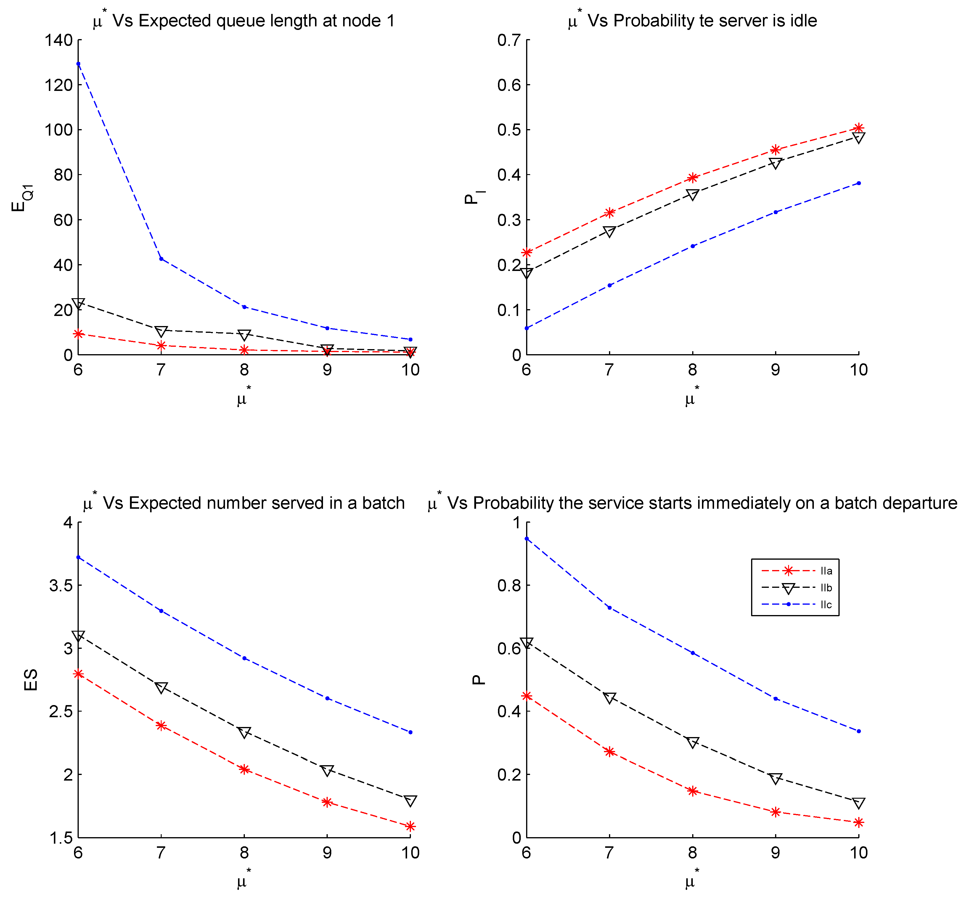
While comparing the performance of queuing systems with different combinations for arrival and service processes, it is imperative that the weighted average service rate or the weighted average service time remains the same in all of the scenarios. This is achieved by normalizing the service rates. Here, we have fixed the weighted average service rates to be ${\mu }^{*}=7$ and ${\mu }^{*}=10$, respectively. The service rates used for various phases and batch sizes when ${\mu }^{*}=10$ in Scenario 1, II, and III are as follows in

Table 8. Service Rates, ${\mu }_j^m$ for various size, m and phase, j in Scenario I.

Phase $\mathit{j},\downarrow$	a			b			c
	m = 2	m = 3	m = 4	m = 2	m = 3	m = 4	m = 2	m = 3	m = 4
1	0.6207	0.9310	1.2414	1	1	1	1.5	1	0.75
2	1.2414	1.8621	2.4828	2	2	2	3	2	1.5
3	1.8621	2.7931	3.7241	3	3	3	4.5	3	2.25
4	2.4828	3.7241	4.9655	4	4	4	6	4	3

,

Table 9. Service Rates, ${\mu }_j^m$ for various batch size, m and phase, j in Scenario II.

Phase $\mathit{j},\downarrow$	a			b			c
	m = 2	m = 3	m = 4	m = 2	m = 3	m = 4	m = 2	m = 3	m = 4
1	1.5517	2.3276	3.1034	2.5	2.5	2.5	3.75	2.5	1.875
2	1.5517	2.3276	3.1034	2.5	2.5	2.5	3.75	2.5	1.875
3	1.5517	2.3276	3.1034	2.5	2.5	2.5	3.75	2.5	1.875
4	1.5517	2.3276	3.1034	2.5	2.5	2.5	3.75	2.5	1.875

and

Table 10. Service Rates, ${\mu }_j^m$ for various batch size, m and phase, j in Scenario III.

Phase $\mathit{j},\downarrow$	a			b			c
	m = 2	m = 3	m = 4	m = 2	m = 3	m = 4	m = 2	m = 3	m = 4
1	2.9793	4.4690	5.9586	4.8	4.8	4.8	7.2	4.8	3.6
2	1.4897	2.2345	2.9793	2.4	2.4	2.4	3.6	2.4	1.8
3	0.9931	1.4897	1.9862	1.6	1.6	1.6	2.4	1.6	1.2
4	0.7448	1.1172	1.4897	1.2	1.2	1.2	1.8	1.2	0.9

:

Based on

Table 11. Measures for various combination of arrival and service processes-Scenario I.

		${\mathit{E}}_{{\mathit{Q}}_1}$	${\mathit{E}}_{{\mathit{Q}}_2}$	${\mathit{E}}_{{\mathit{Q}}_3}$	${\mathit{E}}_{{\mathit{Q}}_4}$	${\mathit{P}}_{\mathit{I}}$	${\mathit{P}}_2$	${\mathit{P}}_3$	${\mathit{P}}_4$	$\mathit{ES}$	P
${\mu }^{*}=7$	$ZCA$ Ia	$2.7302$	$0.8138$	$0.8975$	$1.9219$	$0.0589$	$0.2930$	$0.1925$	$0.4556$	$2.9859$	$0.1532$
	$PCA$ Ia	$17.1330$	$0.9223$	$0.8461$	$1.8747$	$0.1405$	$0.1433$	$0.0723$	$0.6440$	$3.0792$	$0.5646$
	$NCA$ Ia	$3.2177$	$0.8476$	$0.9052$	$1.9300$	$0.1079$	$0.2734$	$0.1392$	$0.4794$	$2.8821$	$0.3036$
	$ZCA$ Ib	$3.8051$	$0.8313$	$0.9021$	$1.9348$	$0.0565$	$0.1729$	$0.1655$	$0.6050$	$3.2626$	$0.2135$
	$PCA$ Ib	$42.1101$	$0.9465$	$0.9597$	$1.9852$	$0.1115$	$0.0656$	$0.0455$	$0.7774$	$3.3772$	$0.7292$
	$NCA$ Ib	$4.3229$	$0.8698$	$0.9142$	$1.9436$	$0.0981$	$0.1529$	$0.1119$	$0.6371$	$3.1898$	$0.4128$
	$ZCA$ Ic	$112.4099$	$0.9919$	$0.9984$	$1.9972$	$0.0025$	$0.0054$	$0.0082$	$0.9839$	$3.9708$	$1.0000$
	$PCA$ Ic	$1743.2$	$0.9651$	$0.9655$	$1.9335$	$0.0038$	$0.0015$	$0.0015$	$0.9601$	$3.8408$	$1.0000$
	$NCA$ Ic	$191.2653$	$0.9943$	$0.9962$	$1.9977$	$0.0042$	$0.0045$	$0.0049$	$0.9864$	$3.9692$	$1.0000$
${\mu }^{*}=10$	$ZCA$ Ia	$1.6573$	$0.7223$	$0.8068$	$1.8811$	$0.1409$	$0.3766$	$0.2021$	$0.2803$	$2.4810$	$0.0448$
	$PCA$ Ia	$3.1906$	$0.8398$	$0.8773$	$1.9517$	$0.3234$	$0.2228$	$0.1076$	$0.3462$	$2.1532$	$0.1996$
	$NCA$ Ia	$1.7587$	$0.7701$	$0.8329$	$1.8981$	$0.2126$	$0.3296$	$0.1509$	$0.3069$	$2.3396$	$0.1134$
	$ZCA$ Ib	$1.3828$	$0.6996$	$0.7763$	$1.8724$	$0.1745$	$0.2795$	$0.2039$	$0.3420$	$2.5388$	$0.0320$
	$PCA$ Ib	$7.0341$	$0.8649$	$0.8887$	$1.9638$	$0.3255$	$0.1270$	$0.0823$	$0.4653$	$2.3619$	$0.3309$
	$NCA$ Ib	$1.6157$	$0.7627$	$0.8181$	$1.8945$	$0.2391$	$0.2294$	$0.1466$	$0.3849$	$2.4383$	$0.1096$
	$ZCA$ Ic	$1.7493$	$0.7295$	$0.7960$	$1.8910$	$0.1608$	$0.1711$	$0.1832$	$0.4842$	$2.8306$	$0.0846$
	$PCA$ Ic	$26.4670$	$0.9126$	$0.9252$	$1.9793$	$0.2304$	$0.0565$	$0.0519$	$0.6612$	$2.9134$	$0.5756$
	$NCA$ Ic	$2.6251$	$0.3043$	$0.8472$	$1.9147$	$0.2002$	$0.1293$	$0.1212$	$0.5494$	$2.8196$	$0.2440$

, the following observations are made:

• Effect of the dependence of service rate on batch size in Scenario 1, on system characteristics: As can be seen from the above Table 8, when the service rate is directly proportional to the stage in which the process is in, the service rate is lowest when the batch size is maximum (for sub-scenario c, service rate is inversely proportional to batch size) (Ic), and this results in an increase in queue length at node 1, $E_{Q_1}$ compared to other combinations of arrival and service processes (Ib and Ia). The server will be serving a bigger batch most of the time as indicated by values of $P_4$ (nearly 1, when ${\mu }^{*}=7$).
• Effect of weighted average service rate on system characteristics: As the weighted average service rate increases (see the rows corresponding to ${\mu }^{*}=7$ and ${\mu }^{*}=10$), the queue length at node 1, $E_{Q_1}$ reduces drastically, and, as a consequence, idle-ness of server, $P_I$ increases significantly. The queue length at other nodes is comparatively less when the weighted average service rate ${\mu }^{*}$ increases (except occasionally for positively correlated arrivals). This could be attributed to customers accessing on-going service from intermediate stages, as the maximum service batch size is not attained in the first stage—or, as the mean number of arrivals to queue 1 during a service time decreases, the queue length at intermediate nodes decreases and vice versa. The number of customers served in a batch ($ES$) and probability that the server serves a batch immediately upon a departure (P) also decreases with the increase in ${\mu }^{*}$.
• Effect of correlation in arrival process on system characteristics: When the arrival process is positively correlated ($PCA$), the queue length at all nodes increases, idle-ness percentage, $P_I$ is maximum, and the server will be serving at its full capacity most of the time compared to other arrival processes (for the same service process).
• Effect of limited waiting room capacity on system characteristics: It is to be noted that the expected values of queue length at all nodes, except the first, did not exceed the waiting room capacity provided at these nodes. The limited waiting room capacity at intermediate nodes does not have a significant impact on system characteristics when the traffic intensity to node 1 increases (As ${\mu }^{*}$ decreases). However if traffic intensity to other nodes increases, there is an increased chance of customers not being able to join the system as maximum waiting room capacity is reached (indicated by higher values of expected queue length to other nodes when ${\mu }^{*}=7$ ).
• Whenever the queue length at node 1, $E_{Q_1}$ increases, the higher the chance to initiate the next batch service immediately (As P increases).

Comparing Table 11 with

Table 12. Measures for various combinations of arrival and service processes—Scenario II.

		${\mathit{E}}_{{\mathit{Q}}_1}$	${\mathit{E}}_{{\mathit{Q}}_2}$	${\mathit{E}}_{{\mathit{Q}}_3}$	${\mathit{E}}_{{\mathit{Q}}_4}$	${\mathit{P}}_{\mathit{I}}$	${\mathit{P}}_2$	${\mathit{P}}_3$	${\mathit{P}}_4$	$\mathit{ES}$	P
${\mu }^{*}=7$	$ZCA$ IIa	$1.4567$	$0.7125$	$0.8017$	$1.8852$	$0.1327$	$0.2440$	$0.2030$	$0.4203$	$2.7784$	$0.0369$
	$PCA$ IIa	$4.0533$	$0.8251$	$0.8839$	$1.9609$	$0.3152$	$0.1274$	$0.0990$	$0.4585$	$2.3856$	$0.2716$
	$NCA$ IIa	$1.6150$	$0.7692$	$0.8319$	$1.9004$	$0.2082$	$0.2085$	$0,1562$	$0.4270$	$2.5938$	$0.1120$
	$ZCA$ IIb	$1.4889$	$0.7233$	$0.8026$	$1.9014$	$0.1321$	$0.1498$	$0.1844$	$0.5337$	$2.9887$	$0.0550$
	$PCA$ IIb	$10.8547$	$0.8853$	$0.9045$	$1.9750$	$0.2765$	$0.0639$	$0.0715$	$0.5882$	$2.6949$	$0.4460$
	$NCA$ IIb	$1.8570$	$0.7874$	$0.8384$	$1.9142$	$0.1976$	$0.1240$	$0.1362$	$0.5422$	$2.8253$	$0.1707$
	$ZCA$ IIc	$2.5770$	$0.8110$	$0.8720$	$1.9477$	$0.0784$	$0.0635$	$0.1237$	$0.7344$	$3.4356$	$0.2039$
	$PCA$ IIc	$42.6360$	$0.9363$	$0.9463$	$1.9884$	$0.1543$	$0.0235$	$0.0392$	$0.7830$	$3.2966$	$0.7282$
	$NCA$ IIc	$4.1035$	$0.8634$	$0.8960$	$1.9500$	$0.1195$	$0.0522$	$0.0867$	$0.7416$	$3.3310$	$0.4463$
${\mu }^{*}=10$	$ZCA$ IIa	$0.9518$	$0.6461$	$0.7061$	$1.8455$	$0.2606$	$0.2626$	$0.1907$	$0.2861$	$2.2417$	$0.0072$
	$PCA$ IIa	$1.1372$	$0.7851$	$0.8182$	$1.9375$	$0.5038$	$0.1443$	$0.1074$	$0.2444$	$1.5887$	$0.0478$
	$NCA$ IIa	$0.9330$	$0.7088$	$0.7602$	$1.8658$	$0.5389$	$0.2171$	$0.1505$	$0.2936$	$2.0599$	$0.0330$
	$ZCA$ IIb	$0.8476$	$0.6390$	$0.6898$	$1.8485$	$0.2876$	$0.1733$	$0.1828$	$0.3562$	$2.32$	$0.0083$
	$PCA$ IIb	$1.7284$	$0.8036$	$0.8308$	$1.9470$	$0.4851$	$0.0835$	$0.0915$	$0.3399$	$1.8011$	$0.1133$
	$NCA$ IIb	$0.9021$	$0.7108$	$0.7540$	$1.8675$	$0.3518$	$0.1400$	$0.1416$	$0.3666$	$2.1712$	$0.0427$
	$ZCA$ IIc	$1.0345$	$0.6658$	$0.7183$	$1.8753$	$0.2462$	$0.1028$	$0.1668$	$0.4847$	$2.6431$	$0.0241$
	$PCA$ IIc	$6.8338$	$0.8593$	$0.8757$	$1.9696$	$0.3811$	$0.0396$	$0.0637$	$0.5156$	$2.3329$	$0.3368$
	$NCA$ IIc	$1.2647$	$0.7450$	$0.7827$	$1.8920$	$0.2971$	$0.0812$	$0.1233$	$0.4978$	$2.5236$	$0.1049$

and

Table 13. Measures for various combination of arrival and service processes—Scenario III.

		${\mathit{E}}_{{\mathit{Q}}_1}$	${\mathit{E}}_{{\mathit{Q}}_2}$	${\mathit{E}}_{{\mathit{Q}}_3}$	${\mathit{E}}_{{\mathit{Q}}_4}$	${\mathit{P}}_{\mathit{I}}$	${\mathit{P}}_2$	${\mathit{P}}_3$	${\mathit{P}}_4$	$\mathit{ES}$	P
${\mu }^{*}=7$	$ZCA$ IIIa	$2.0173$	$0.7802$	$0.8559$	$1.9318$	$0.0845$	$0.1054$	$0.1452$	$0.6649$	$3.3061$	$0.1397$
	$PCA$ IIIa	$14.3871$	$0.9022$	$0.9206$	$1.9810$	$0.2176$	$0.0479$	$0.0648$	$0.6697$	$2.9688$	$0.5506$
	$NCA$ IIIa	$2.5465$	$0.8284$	$0.8744$	$1.9355$	$0.1429$	$0.0931$	$0.1175$	$0.6465$	$3.1248$	$0.3056$
	$ZCA$ IIIb	$3.0283$	$0.8445$	$0.9001$	$1.9610$	$0.0547$	$0.0435$	$0.0932$	$0.8087$	$3.6012$	$0.2947$
	$PCA$ IIIb	$39.2096$	$0.9365$	$0.9477$	$1.9901$	$0.1418$	$0.0190$	$0.0389$	$0.8003$	$3.3559$	$0.7589$
	$NCA$ IIIb	$4.3710$	$0.8819$	$0.9116$	$1.9610$	$0.0951$	$0.0392$	$0.0751$	$0.7905$	$3.4659$	$0.5518$
	$ZCA$ IIIc	$106.6966$	$0.9949$	$0.9971$	$1.9960$	$0.0014$	$0.0008$	$0.0028$	$0.9950$	$3.9901$	$1.0000$
	$PCA$ IIIc	$1734.5$	$0.9634$	$0.9658$	$1.9345$	$0.0041$	$0.0003$	$0.0012$	$0.9617$	$3.8511$	$1.0000$
	$NCA$ IIIc	$185.6821$	$0.9961$	$0.9972$	$1.9999$	$0.0027$	$0.0007$	$0.0023$	$0.9941$	$3.9851$	$1.0000$
${\mu }^{*}=10$	$ZCA$ IIIa	$1.1550$	$0.6797$	$0.7433$	$1.8911$	$0.2000$	$0.1353$	$0.1726$	$0.4921$	$2.7569$	$0.0326$
	$PCA$ IIIa	$2.4595$	$0.8254$	$0.8522$	$1.9613$	$0.4115$	$0.0659$	$0.0867$	$0.4359$	$2.1354$	$0.1892$
	$NCA$ IIIa	$1.2588$	$0.7448$	$0.7899$	$1.9003$	$0.2744$	$0.1137$	$0.1369$	$0.4750$	$2.5381$	$0.1004$
	$ZCA$ IIIb	$1.3270$	$0.7076$	$0.7678$	$1.9132$	$0.1741$	$0.0740$	$0.1439$	$0.6080$	$3.0117$	$0.0596$
	$PCA$ IIIb	$6.6041$	$0.8648$	$0.8823$	$1.9759$	$0.3430$	$0.0313$	$0.0618$	$0.5639$	$2.5037$	$0.3674$
	$NCA$ IIIb	$1.5882$	$0.7737$	$0.8103$	$1.9194$	$0.2385$	$0.0622$	$0.1127$	$0.5866$	$2.8088$	$0.1742$
	$ZCA$ IIIc	$2.2616$	$0.7964$	$0.8506$	$1.9521$	$0.0977$	$0.0303$	$0.0929$	$0.7792$	$3.4559$	$0.1949$
	$PCA$ IIIc	$25.8120$	$0.9165$	$0.9274$	$1.9884$	$0.2081$	$0.0123$	$0.0370$	$0.7426$	$3.1060$	$0.6457$
	$NCA$ IIIc	$3.1082$	$0.8479$	$0.8741$	$1.9537$	$0.1445$	$0.0262$	$0.0727$	$0.7567$	$3.2972$	$0.4298$

the following observations are made:

• Effect of the dependence of service rate on the stage (in which the process is in): Comparing Table 9 with Table 8 and Table 10, one could see that, when the service rate remains constant for stages, i.e., in Scenario II, the individual service rates are comparatively stable. This is reflected in performance measures given in Table 12 compared to that given in Table 11 and Table 13. The queuing system becomes more stable. The queue length at node 1 decreases drastically while, at other nodes, it is more or less the same. Another interesting feature is that the performance measures are more or less the same in Scenario I and Scenario III (i.e, when the service rate is inversely proportional to the phase in which the process is in).
• All observations made in the above paragraph regarding the behavior of the system for various combinations of arrival and service processes in Scenario I remains valid in Scenarios II and III, as can be seen from tables and graphs plotted in Figure 2.

6. Cost Analysis

Here, we present cost analysis for the queuing system considered in the above example. The service rate depends on the stage and the number in service at that time. The objective of this section is to study the effect of this dependence on cost incurred per unit time.

The server operates from stage 1 to the destination, so we do not attribute a cost with regard to the phase from which a customer joins. If we are to consider a revenue function, this has to be taken into account. However, we impose a penalty when the system is not operating to its full capacity by saying that the cost of offering service is higher when this happens. Based on the performance measures, we define a cost function, cost per unit time as

$$C=\sum _{j=1}^{j=4}{C}_{Q_j}\times E_{Q_j}+C_{P_I}\times P_I+\sum _{m=2}^4{C}_m\times P_m,$$

where

$C_{Q_j}:$ Holding cost for retaining a customer in queue at node j per unit time

$C_{P_I}:$ Cost incurred due to server idleness per unit time

$C_m:$ Cost per unit time for offering service to a batch of size m.

Here, we assume $C_{Q_1}=1,C_{Q_2}=C_{Q_3}=C_{Q_4}=0.5,C_{P_I}=2,C_2=15,C_3=12.5,$$C_4=10.$

From

Table 14. Cost per unit time in Scenario I.

Arrival Process ↓	${\mathit{\mu }}^{*}=7$			${\mathit{\mu }}^{*}=10$
	Ia	Ib	Ic	Ia	Ib	Ic
$ZCA$	16.0216	$\mathbf{15}.\mathbf{7456}$	124.4203	14.6238	13.5680	13.4861
$PCA$	28.8277	53.6053	1754.7	13.8211	17.1296	36.9443
$NCA$	15.9107	16.4458	203.262	13.8339	$\mathbf{12}.\mathbf{9520}$	13.7563

,

Table 15. Cost per unit time in Scenario II.

Arrival Process ↓	${\mathit{\mu }}^{*}=7$			${\mathit{\mu }}^{*}=10$
	Ia	Ib	Ic	Ia	Ib	Ic
$ZCA$	13.8224	13.3561	14.3902	11.3508	11.4847	12.2555
$PCA$	14.2647	21.0234	53.5530	$\mathbf{9}.\mathbf{8673}$	10.2841	15.9950
$NCA$	13.1329	$\mathbf{13}.\mathbf{0063}$	15.3906	11.3508	10.8084	11.3076

and

Table 16. Cost per unit time in Scenario III.

Arrival Process ↓	${\mathit{\mu }}^{*}=7$			${\mathit{\mu }}^{*}=10$
	Ia	Ib	Ic	Ia	Ib	Ic
$ZCA$	14.0155	14.8940	118.6923	12.3201	12.3580	13.6631
$PCA$	24.9499	49.2046	1746	$\mathbf{11.5330}$	16.0326	36.2175
$NCA$	$\mathbf{13.9819}$	15.8713	197.666	11.6914	12.0246	14.1749

, it can be seen that the cost is lower for all combinations of arrival and service processes in Scenario II (service rate is constant with respect to stages) compared to corresponding costs in Scenarios I and III. The cost is higher if the arrival process is positively correlated except in sub-scenario a. (corresponding to ${\mu }^{*}=10$) i.e., the service rate is directly proportional to batch size. This could be attributed to a drastic increase in queue length for positively correlated arrivals. As expected, the increase in weighted average service rate decreases in cost as the number served per unit time increases. When arrivals are positively correlated, the cost increases when the rate is inversely proportional to batch size. (i.e., in sub-scenario c). The minimum cost in each of the Scenarios and Sub-scenarios are indicated in bold font. Though the costs are input specific, it gives a general picture.

7. Conclusions

In this paper, we have analyzed a queuing system with k stages of service with the customer having the choice to join a service from the beginning of any of the stages. Another key feature of the model is that the service rate at each stage depends on the stage as well as the number of customers served in a batch. The performance measures for such a system are computed and an illustrative numerical example is provided. A cost function is constructed based on performance measures, and an analysis to study the effect of service rates under various scenarios to this cost function is presented.

Several variants of the queueing model considered in this paper are proposed to be analyzed in the future. In the introduction, we have indicated two such future directions of research, directly related to this paper. In addition, we propose to examine the admission of fresh customers to an on-going service on expiry of a random duration, which is generally distributed. This could be done at several such realization epochs. Another variant is the case of customers not only having access to an ongoing service, but also alighting at intermediate nodes during the transport vehicle moving forward as well as in the reverse direction.

References

- Banerjee, A.; Gupta, U.C.; Chakravarthy, S.R. Analysis of a finite-buffer bulk-service queue under Markovian arrival process with batch-size dependent service. Comput. Oper. Res. 2015, 60, 138–149. [Google Scholar] [CrossRef]
- D’Arienzo, M.P.; Dudin, A.N.; Dudin, S.A.; Manzo, R. Analysis of a retrial queue with group service of impatient customers. J. Ambient. Intell. Humaniz. Comput. 2019. [Google Scholar] [CrossRef]
- Neuts, M.F. A General Class of Bulk Queues with Poisson Input. Ann. Math. Stat. 1967, 38, 759–770. [Google Scholar] [CrossRef]
- Sivasamy, R. A bulk service queue with accessible and non-accessible batches. Opsearch 1990, 27, 46–54. [Google Scholar]
- Ayappan, G.; Renganathan, N. A preemptive priority queue with accessible batch services and heterogeneous arrivals. Inf. Manag. Sci. 1997, 8, 63–72. [Google Scholar]
- Baburaj, C.; Manoharan, M. On a Markovian single and batch service queue with accessibility. Int. J. Inf. Manag. Sci. 1999, 10, 17–23. [Google Scholar]
- Krishnamoorthy, A.; Ushakumari, P.V. A queueing system with single arrival bulk service and single departure. Math. Comput. Model. 2000, 31, 99–108. [Google Scholar] [CrossRef]
- Baburaj, C. On the transient distribution of a single and batch service queueing system with accessibility to batches. Inf. Manag. Sci. 2000, 11, 27–36. [Google Scholar]
- Baburaj, C. A controllable bulk service queueing system with accessible and non accessible batches. Inf. Manag. Sci. 2002, 13, 83–89. [Google Scholar]
- Baburaj, C. An (a, c, d) policy bulk service queue with accessible and non-accessible batches. J. Kerala Stat. Assoc. 2006, 17, 10–20. [Google Scholar]
- Goswami, V.; Vijaya Laxmi, P. A renewal input single and batch service queues with accessibility to batches. Int. J. Manag. Sci. Eng. Manag. 2011, 6, 366–373. [Google Scholar] [CrossRef]
- Goswami, V.; Vijaya Laxmi, P. Performance Analysis of a Renewal Input Bulk Service Queue with Accessible and Non-Accessible Batches. Qual. Technol. Quant. Manag. 2011, 8, 87–100. [Google Scholar] [CrossRef]
- Gupta, U.C.; Goswami, V. Performance analysis of finite buffer discrete time queue with bulk service. Comput. Oper. Res. 2002, 29, 1331–1341. [Google Scholar] [CrossRef]
- Goswami, V.; Mohanty, J.R.; Samanta, S.K. Discrete-time bulk-service queues with accessible and non-accessible batches. Appl. Math. Comput. 2006, 182, 898–906. [Google Scholar] [CrossRef]
- Goswami, V.; Samanta, S.K. Discrete-Time Single and Batch Service Queues with Accessibility to the Batches. Int. J. Inf. Manag. Sci. 2009, 20, 27–38. [Google Scholar]
- Sivasamy, R.; Pukazhenthi, N. A Discrete time bulk service queue with accessible batch: Geo/NBL,K/1. Opsearch 2009, 46, 321–334. [Google Scholar] [CrossRef]
- Goswami, V.; Sikdar, K. Discrete-time batch service GI/Geo/1/N queue with accessible and non-accessible batches. Int. J. Math. Oper. Res. 2010, 2, 233–257. [Google Scholar] [CrossRef]
- Jain, M.; Agrawal, P.K. Discrete time analysis of state dependent batch service queue with balking, accessible and non accessible batches. Math. Today 2010, 26, 28–39. [Google Scholar]
- Goswami, V.; Vijaya Laxmi, P. Discrete time renewal input multiple vacation queue with accessible and non-accessible batches. Opsearch 2011, 48, 335–354. [Google Scholar] [CrossRef]
- Baburaj, C.; Rekha, P. A discrete time (a, c, d) policy bulk service queue with accessible and non accessible batches. J. Kerala Stat. Assoc. 2015, 25, 33–50. [Google Scholar]
- Vijaya Laxmi, P.; Goswami, V.; Yesuf, O.M. Finite buffer renewal input multiple exponential vacations queue with accessible and non-accessible batches. Int. J. Manag. Sci. Eng. Manag. 2010, 5, 227–234. [Google Scholar]
- Vijaya Laxmi, P.; Yesuf, O.M. Renewal input infinite buffer batch service queue with single exponential working vacation and accessibility to batches. Int. J. Math. Oper. Res. 2011, 3. [Google Scholar] [CrossRef]
- Ayappan, G.; Sridevi, S. Bulk service Markovian queue with service batch size dependent and accessible and non accessible batches and with vacation. J. Comput. Model. 2012, 2, 123–135. [Google Scholar]
- Balasubramanian, M. Steady state analysis of a bulk queueing model with multiple vacations, accessible batches and closedown times. Bonfring Int. J. Eng. Manag. Sci. 2013, 3, 118–127. [Google Scholar]
- Sridhar, A.; Pitchai, R.A. Two server queueing system with single and batch service. Int. J. Appl. Oper. Res. 2014, 4, 15–26. [Google Scholar]
- Neuts, M.F. Matrix Geometric Solutions in Stochastic Models: An Algorithmic Approach; The Johns Hopkins University Press: Baltimore, MD, USA, 1981. [Google Scholar]
Figure 1.
Queueing system with four stages of service, with accessibility to service from the beginning of any stage.