The Impact of Model Uncertainty on Index-Based Longevity Hedging and Measurement of Longevity Basis Risk

Abstract

We investigate the impact of model uncertainty on hedging longevity risk with index-based derivatives and assessing longevity basis risk, which arises from the mismatch between the hedging instruments and the portfolio being hedged. We apply the bivariate Lee–Carter model, the common factor model, and the M7-M5 model, with separate cohort effects between the two populations, and various time series processes and simulation methods, to build index-based longevity hedges and measure the hedge effectiveness. Based on our modeling and simulations on hypothetical scenarios, the estimated levels of hedge effectiveness are around 50% to 80% for a large pension plan, and the model selection, particularly in dealing with the computed time series, plays a very important role in the estimation. We also experiment with a modified bootstrapping approach to incorporate the uncertainty of model selection into the modeling of longevity basis risk. The hedging results under this approach may approximately be seen as a “weighted” average of those calculated from the different model candidates.

1. Introduction

Continual increase in longevity worldwide remains a serious concern for pension plan sponsors and annuity providers. The major issue is the presence of longevity risk, which is the risk of paying more than expected because of unanticipated mortality improvements. Broadly speaking, there are three ways to mitigate longevity risk (e.g., Cairns et al. 2008). The first is to transfer the unwanted risk to an insurer or reinsurer by paying a premium. The problem of this usual approach is that insurers and reinsurers may also have limited appetite, and that a failure of a major player could cause disastrous systemic outcomes. The second way is natural hedging, which makes use of the opposite movements between the values of annuities and life insurances arising from changes in mortality levels (e.g., Li and Haberman 2015). Although certain large institutions may have the resources and economies of scale to offer both lines of products and so exploit this hedging effect, many other financial entities do not have such necessary conditions to follow suit.

The third way is the use of capital market solutions, such as insurance securitization (e.g., Cowley and Cummins 2005), and mortality- and longevity-linked securities (e.g., LCP 2012; Coughlan et al. 2007). The former involves packaging insurance and business risks into securities, such as bonds with coupon and principal payments depending on the performance of the underlying portfolio. The latter has two types of transactions, bespoke and index-based. Bespoke transactions are tailored to individual circumstances, for example, pension buy-ins, buy-outs, and longevity swaps. In contrast, index-based solutions are constructed such that the cashflows are linked to the values of selected mortality indices. As noted in Zhou and Li (2016), there is an imbalance between demand and supply in longevity risk transfer. The insurance industry alone cannot generate sufficient supply for accepting the risk due to capital constraints. Accordingly, an important, recent idea is to design standardized products based on well-specified mortality indices, in order to draw more investors’ interest and develop market liquidity.

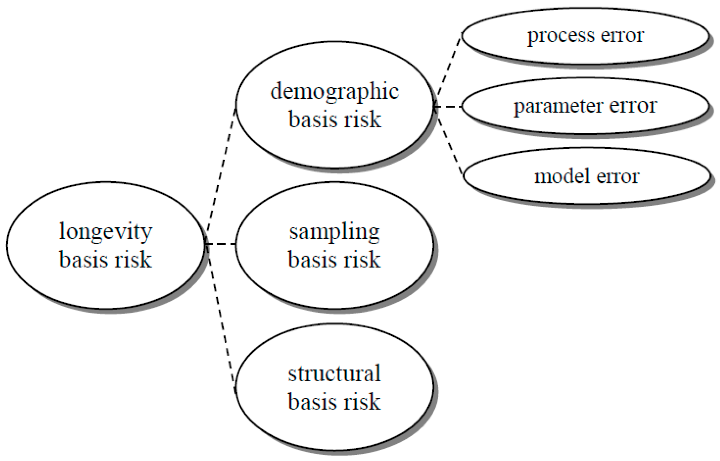
One significant challenge in implementing index-based hedging in practice is the existence of longevity basis risk, i.e., there is a mismatch or discrepancy between the hedging instruments (linked to a reference population) and the pension or annuity portfolio being hedged (with the underlying book population). Haberman et al. (2014) established a mortality modeling framework incorporating three fundamental sources of longevity basis risk. They include demographic basis risk which comes from demographic or socioeconomic differences between the book and reference populations, sampling basis risk due to the randomness of outcomes of individual lives, and structural basis risk in terms of how the payoff structures differ between the hedging instruments and the portfolio to be hedged. Li et al. (2017) then adopted the framework and focused on assessing longevity basis risk in realistic scenarios under practical circumstances. The major finding is that for a large portfolio, about 50% to 80% of its longevity risk can often be reduced via index-based longevity swaps, while for a small portfolio, the risk reduction is usually less than 50%.

In particular, from a modeling viewpoint, or a regulatory perspective such as Solvency II (CEIOPS 2010), demographic basis risk can further be divided into process error, parameter error, and model error (or process risk, parameter uncertainty, model uncertainty, respectively). Process error refers to the variability in the time series, parameter error arises from the uncertainty in estimating model parameters, and model error reflects the uncertainty in model selection. Figure 1 below provides a graphical summary of all these risk components. Although several authors proposed different ways to allow for both process error and parameter error in index-based hedging (e.g., Li and Luo 2012; Cairns 2013; Tan et al. 2014; Haberman et al. 2014), relatively little attention has been given to assessing model error. Most of the studies covered process error only or considered both process error and parameter error, while some compared the hedging results briefly between a few different mortality projection models. Li et al. (2016) took a step further by examining the effectiveness of a hedging strategy based on a particular model but under a simulated environment produced from another model, and found that coherence is a critical assumption in measuring the hedge effectiveness. Li et al. (2017) conducted a detailed sensitivity analysis by changing various modeling assumptions. They noted that the most important ones were the coherence property, behavior of simulated future variability, simulation method, and additional model features such as structural mortality changes.

In this paper, we perform a more elaborate investigation on model error in an attempt to supplement the current literature from two perspectives. Firstly, we assess the hedge effectiveness based on three broad “families” of mortality projection models, a range of time series processes under each model, and several simulation methods for each combination. Many of these combinations have not been tested or studied in detail in the literature. Secondly, we adopt the modified semi-parametric bootstrapping approach in Yang et al. (2015) and incorporate all the three errors in an integrated manner. From these two different perspectives, we attempt to obtain better insights into the potential impact of selecting an inappropriate model in hedging longevity risk with index-based solutions.

This paper is organized as follows. In Section 2, we set forth a list of two-population mortality projection models, time series processes, and simulation approaches selected for our analysis. In Section 3, we examine the hedge effectiveness under different model settings and assumptions and simulated scenarios, and provide a discussion on the impact of model uncertainty. Finally, we give our concluding remarks and set forth some suggestions for future research in Section 4.

2. Mortality Modeling and Simulations

Recently, there is an emerging branch of literature that focuses on modeling multiple populations jointly. Haberman et al. (2014) and Li et al. (2014) provide a comprehensive review of several multi-population mortality projection models for measuring longevity basis risk. Although there are probably more than 30 models proposed in the literature, we select the ones below for our analysis, as they can be deemed as “key representatives” of the major “families” of mortality projection models.

The first belongs to the Lee and Carter (1992) family, in which there are some possible options (noted as Model 1a, Model 1b, Model 1c, and Model 1d respectively) for modeling the time-varying parameters:

$$\begin{array}{ll}\ln m_{x,t,i}={\alpha }_{x,i}+{\beta }_{x,i}{\mathit{\kappa }}_{t,i}+{\mathit{\iota }}_{t-x,i};& (\mathrm{Lee}–\mathrm{Carter}\mathrm{model}\mathrm{with}\mathrm{cohort})\end{array}$$

(1)

with

$$\begin{array}{ll}{\mathrm{K}}_t=\Theta +{\mathrm{K}}_{t-1}+{\Delta }_t,& \left(\mathrm{bivariate}\mathrm{random}\mathrm{walk}\mathrm{with}\mathrm{drift}\right)\end{array}$$

(1a)

or

$$\begin{array}{ll}{\mathit{\kappa }}_{t,1}=\theta +{\mathit{\kappa }}_{t-1,1}+{\delta }_t,& \left(\mathrm{random}\mathrm{walk}\mathrm{with}\mathrm{drift}\right)\\ {\mathit{\kappa }}_{t,2}=a_0+a_1{\mathit{\kappa }}_{t,1}+{\omega }_t,& (\mathrm{co}-\mathrm{integrated}\mathrm{process})\end{array}$$

(1b)

or

$$\begin{array}{ll}{\mathrm{K}}_t-{\mathrm{K}}_{t-1}=\Theta +\Pi {\mathrm{K}}_{t-1}+{\displaystyle \sum _{r=1}^{p-1}{\Gamma }_r\left({\mathrm{K}}_{t-r}-{\mathrm{K}}_{t-r-1}\right)}+{\Delta }_t,& \left(\mathrm{VECM}\right(p\left)\right)\end{array}$$

(1c)

or

$$\begin{array}{ll}{\mathrm{K}}_t-{\mathrm{K}}_{t-1}=\Theta +{\displaystyle \sum _{r=1}^p{\Gamma }_r\left({\mathrm{K}}_{t-r}-{\mathrm{K}}_{t-r-1}\right)}+{\Delta }_t.& \left(\mathrm{VARIMA}\right(p,1,0\left)\right)\end{array}$$

(1d)

The term $m_{x,t,i}$ is the central death rate at age $x$ in year $t$ of population $i$, in which $i=1$ refers to the reference population and $i=2$ refers to the book population. The parameter ${\alpha }_{x,i}$ is the general age schedule, ${\mathit{\kappa }}_{t,i}$ is the mortality index over time, ${\mathrm{K}}_t=\left({\mathit{\kappa }}_{t,1},{\mathit{\kappa }}_{t,2}\right)\prime$, and ${\beta }_{x,i}$ is the age sensitivity of the log death rate to the mortality index. The cohort parameter ${\mathit{\iota }}_{t-x,i}$ is added when there are significant patterns in the residuals against cohort year (e.g., Haberman and Renshaw 2011). It can be modeled with an autoregressive integrated moving average (ARIMA) process for future projections and simulations, though this is not required in the analysis in the next section. Following Cairns et al. (2009), the first and last five cohorts are excluded from the fitting procedure due to a lack of data.

The first method suggested in Carter and Lee (1992) is fitting the Lee–Carter model to each population separately and then modeling the relationship between the two resulting mortality indices. This approach involves the use of a bivariate random walk with drift (1a) naturally, in which $\Theta$ is the vector drift term and ${\Delta }_t$ is the Gaussian vector error term. In contrast, the third method in Carter and Lee (1992) is treating the two mortality indices as a co-integrated process (1b), where $\theta$, $a_0$, and $a_1$ are the parameters of the process, and ${\delta }_t$ and ${\omega }_t$ are independent Gaussian error terms. Moreover, Yang and Wang (2013) proposed using a vector error correction model (VECM) of order $p$ (1c), in which $\Theta$ is the vector constant term, $\Pi$ and ${\Gamma }_r$ are the matrix components, and ${\Delta }_t$ is the Gaussian vector error term. Finally, we also consider a vector autoregressive integrated moving average (VARIMA) process (1d), which has been explored by Chan et al. (2014) in modeling other mortality indices. The order chosen is ($p$, 1, 0), $\Theta$ is the vector constant term, ${\Gamma }_r$ is the autoregressive matrix, and ${\Delta }_t$ is the Gaussian vector error term. The VARIMA in (1d) is in line with the VECM in (1c) and serves as an extension of the random walk in (1a) and (1b) in terms of allowing for more flexibility in modeling the various mortality indices, for comparison purposes. Please note that all the options (1a) to (1d) would generally lead to non-coherence in mortality projections, i.e., the ratio of projected death rates (central estimates) between the two populations at each age group does not converge to a constant over time (e.g., Cairns et al. 2011).

The second is the Li and Lee (2005) family, which is an extension of the Lee–Carter model and assumes a common factor for the two populations. Again, there are a few possible choices (noted as Model 2a, Model 2b, Model 2c, and Model 2d respectively) in modeling the temporal parameters:

$$\begin{array}{ll}\ln m_{x,t,i}={\alpha }_{x,i}+{\beta }_x^c{\mathit{\kappa }}_t^c+{\displaystyle \sum _{j=1}^n{\beta }_{x,i,j}{\mathit{\kappa }}_{t,i,j}}+{\mathit{\iota }}_{t-x,i},& \left(\mathrm{generalized}\mathrm{common}\mathrm{factor}\mathrm{model}\mathrm{with}\mathrm{cohort}\right)\\ {\mathit{\kappa }}_t^c=d+{\mathit{\kappa }}_{t-1}^c+{\epsilon }_t;& \left(\mathrm{random}\mathrm{walk}\mathrm{with}\mathrm{drift}\right)\end{array}$$

(2)

with

$$\begin{array}{ll}{\mathit{\kappa }}_{t,i,j}={\theta }_{i,j}+{\gamma }_{1,i,j}{\mathit{\kappa }}_{t-1,i,j}+{\delta }_{t,i,j},& \left(\mathrm{AR}\right(1);\mathrm{independent}{\delta }_{t,1,j}\mathrm{and}{\delta }_{t,2,j})\end{array}$$

(2a)

or

$$\begin{array}{ll}{\mathit{\kappa }}_{t,i,j}={\theta }_{i,j}+{\displaystyle \sum _{r=1}^p{\gamma }_{r,i,j}{\mathit{\kappa }}_{t-r,i,j}}+{\delta }_{t,i,j},& \left(\mathrm{AR}\right(p);\mathrm{independent}{\delta }_{t,1,j}\mathrm{and}{\delta }_{t,2,j})\end{array}$$

(2b)

or

$$\begin{array}{ll}{\mathit{\kappa }}_{t,i,j}={\theta }_{i,j}+{\displaystyle \sum _{r=1}^p{\gamma }_{r,i,j}{\mathit{\kappa }}_{t-r,i,j}}+{\delta }_{t,i,j},& \left(\mathrm{AR}\right(p);\mathrm{correlated}{\delta }_{t,1,j}\mathrm{and}{\delta }_{t,2,j})\end{array}$$

(2c)

or

$$\begin{array}{ll}{\mathrm{K}}_{t,j}={\Theta }_j+{\displaystyle \sum _{r=1}^p{\Gamma }_{r,j}{\mathrm{K}}_{t-r,j}}+{\Delta }_{t,j}.& \left(\mathrm{VAR}\right(p\left)\right)\end{array}$$

(2d)

The parameter ${\alpha }_{x,i}$ is the general age schedule of population $i$, ${\mathit{\kappa }}_t^c$ is the mortality index of the common factor for both populations with age sensitivity ${\beta }_x^c$, and ${\mathit{\kappa }}_{t,i,j}$ is the time component of the jth additional factor for population $i$ with age sensitivity ${\beta }_{x,i,j}$. The common mortality index is modeled as a random walk with drift as usual, with $d$ as the drift and ${\epsilon }_t$ as the Gaussian error. Originally, Li and Lee (2005) used only one additional factor; later, Li (2013) proposed using $n$ additional factors where necessary, and Yang et al. (2016) further suggested adding different cohort parameters such as ${\mathit{\iota }}_{t-x,i}$.

Li and Lee (2005) assumed that ${\mathit{\kappa }}_{t,i,1}$ followed an autoregressive (AR) process of order one, and that the error terms are independent between the populations (2a). On the other hand, Li (2013) tested a more general AR($p$) process for each ${\mathit{\kappa }}_{t,i,j}$ (2b), and Zhou and Li (2016) assumed that the error terms ${\delta }_{t,i,1}$’s are correlated between the populations (2c). The parameters ${\theta }_{i,j}$ and ${\gamma }_{r,i,j}$ are the constant and autoregressive terms respectively. Lastly, we also include a vector autoregressive (VAR) process of order $p$ for ${\mathrm{K}}_{t,j}=\left({\mathit{\kappa }}_{t,1,j},{\mathit{\kappa }}_{t,2,j}\right)\prime$ (2d), which has been adopted by Haberman et al. (2014) for modeling some other mortality indices. The notation ${\Theta }_j$ is the vector constant term, ${\Gamma }_{r,j}$ is the autoregressive matrix, and ${\Delta }_{t,j}$ is the Gaussian vector error term. All the choices (2a) to (2d) can result in coherence in mortality projections, i.e., the ratio of projected death rates between the two populations at each age group tends to a constant over time, if the selected time series processes are weakly stationary. More technical details of time series modeling can be found in Tsay (2002).

The final one is an extension of the Cairns-Blake-Dowd (CBD) model by Cairns et al. (2006) and is proposed by Haberman et al. (2014), being referred to as the M7-M5 model. There are also several possible time series processes to choose from (noted as Model 3a, Model 3b, Model 3c, and Model 3d respectively) under this model:

$$\begin{array}{ll}\mathrm{logit}{q}_{x,t}^R={\mathit{\kappa }}_{t,1}^R+\left(x-\overline{x}\right){\mathit{\kappa }}_{t,2}^R+\left({\left(x-\overline{x}\right)}^2-{\sigma }_{}^2\right){\mathit{\kappa }}_{t,3}^R+{\mathit{\iota }}_{t-x}^R,& \left(\mathrm{extended}\mathrm{CBD}\mathrm{model}\mathrm{with}\mathrm{cohort}\right)\\ \mathrm{logit}{q}_{x,t}^B-\mathrm{logit}{q}_{x,t}^R={\mathit{\kappa }}_{t,1}^B+\left(x-\overline{x}\right){\mathit{\kappa }}_{t,2}^B+{\mathit{\iota }}_{t-x}^B& \left(\mathrm{CBD}\mathrm{model}\mathrm{structure}\mathrm{with}\mathrm{cohort}\right)\end{array}$$

(3)

with

$$\begin{array}{ll}{\mathrm{K}}_t^R={\Theta }^R+{\mathrm{K}}_{t-1}^R+{\Delta }_t^R,& \left(\mathrm{multivariate}\mathrm{random}\mathrm{walk}\mathrm{with}\mathrm{drift}\right)\\ {\mathrm{K}}_t^B={\Theta }^B+{\displaystyle \sum _{r=1}^p{\Gamma }_r^B{\mathrm{K}}_{t-r}^B}+{\Delta }_t^B,& \left(\mathrm{VAR}\right(p);\mathrm{independent}{\Delta }_t^R\mathrm{and}{\Delta }_t^B)\end{array}$$

(3a)

or

$$\begin{array}{ll}{\mathrm{K}}_t^R-{\mathrm{K}}_{t-1}^R={\Theta }^R+{\displaystyle \sum _{r=1}^p{\Gamma }_r^R\left({\mathrm{K}}_{t-r}^R-{\mathrm{K}}_{t-r-1}^R\right)}+{\Delta }_t^R,& \left(\mathrm{VARIMA}\right(p,1,0\left)\right)\\ {\mathrm{K}}_t^B={\Theta }^B+{\displaystyle \sum _{r=1}^p{\Gamma }_r^B{\mathrm{K}}_{t-r}^B}+{\Delta }_t^B,& \left(\mathrm{VAR}\right(p);\mathrm{independent}{\Delta }_t^R\mathrm{and}{\Delta }_t^B)\end{array}$$

(3b)

or

$$\begin{array}{ll}{\mathrm{K}}_t^R={\Theta }^R+{\mathrm{K}}_{t-1}^R+{\Delta }_t^R,& \left(\mathrm{multivariate}\mathrm{random}\mathrm{walk}\mathrm{with}\mathrm{drift}\right)\\ {\mathrm{K}}_t^B={\mathrm{K}}_{t-1}^B+{\Delta }_t^B,& (\mathrm{bivariate}\mathrm{random}\mathrm{walk}\mathrm{without}\mathrm{drift};\mathrm{independent}{\Delta }_t^R\mathrm{and}{\Delta }_t^B)\end{array}$$

(3c)

or

$$\begin{array}{ll}{\mathrm{K}}_t^R={\Theta }^R+{\mathrm{K}}_{t-1}^R+{\Delta }_t^R,& \left(\mathrm{multivariate}\mathrm{random}\mathrm{walk}\mathrm{with}\mathrm{drift}\right)\\ {\mathrm{K}}_t^B={\Theta }^B+{\displaystyle \sum _{r=1}^p{\Gamma }_r^B{\mathrm{K}}_{t-r}^B}+{\Delta }_t^B.& \left(\mathrm{VAR}\right(p);\mathrm{correlated}{\Delta }_t^R\mathrm{and}{\Delta }_t^B)\end{array}$$

(3d)

The term $q_{x,t}^R$ is the mortality rate at age $x$ in year $t$ of the reference population, ${\mathit{\kappa }}_{t,1}^R$, ${\mathit{\kappa }}_{t,2}^R$, and ${\mathit{\kappa }}_{t,3}^R$ represent the level, slope, and curvature of the mortality curve in year $t$ (e.g., Cairns et al. 2009), and ${\mathit{\iota }}_{t-x}^R$ is the cohort parameter. The difference in the logit mortality rate between the book and reference populations (i.e., $\mathrm{logit}{q}_{x,t}^B-\mathrm{logit}{q}_{x,t}^R$) is then modeled with another CBD structure of ${\mathit{\kappa }}_{t,1}^B$ and ${\mathit{\kappa }}_{t,2}^B$, which explain the differences between the two populations, together with another cohort parameter ${\mathit{\iota }}_{t-x}^B$. Please note that the original M7-M5 model has a common cohort parameter for both populations, while we use a separate cohort parameter for each population in order to allow for the different cohort effects in our data. The notation $\overline{x}$ is the average age of the age range in the data, and ${\sigma }_{}^2$ is the average value of ${\left(x-\overline{x}\right)}^2$.

In contrast to families (1) and (2) above, where both populations are modeled in parallel, Haberman et al. (2014) fitted the reference population first and then the differences between the two populations. One major argument for this treatment is that there are usually much more data for the reference population than for the book, and so it would be more appropriate to base the main trends on the reference population and consider the differences of the book population afterwards.

Haberman et al. (2014) assumed that ${\mathrm{K}}_t^R=\left({\mathit{\kappa }}_{t,1}^R,{\mathit{\kappa }}_{t,2}^R,{\mathit{\kappa }}_{t,3}^R\right)\prime$ follows a multivariate random walk with drift, ${\mathrm{K}}_t^B=\left({\mathit{\kappa }}_{t,1}^B,{\mathit{\kappa }}_{t,2}^B\right)\prime$ follows a VAR(1) process, and ${\Delta }_t^R$ and ${\Delta }_t^B$ are independent, whereas we adopt a more general VAR($p$) process here for ${\mathrm{K}}_t^B$ (3a). Accordingly, we also consider three other alternatives. First, similar to replacing the option (1a) with (1d), we replace the multivariate random walk with drift with a VARIMA($p$, 1, 0) process for ${\mathrm{K}}_t^R$ (3b). Second, we replace the VAR($p$) process with a bivariate random walk without drift for ${\mathrm{K}}_t^B$ (3c), as we have seen in our analysis that the calculated ${\mathit{\kappa }}_{t,1}^B$ and ${\mathit{\kappa }}_{t,2}^B$ fluctuate around a constant level in many cases. Moreover, in line with the options (2b) and (2c), we test the correlation assumption between ${\Delta }_t^R$ and ${\Delta }_t^B$ (3d). All the vectors and matrices of parameters and error terms have similar meanings as previously. Please note that the options (3a), (3b) and (3d) can generate coherence in the projected mortality rates approximately if the selected VAR process is weakly stationary.

Besides the central estimates’ coherence, the simulated future variability is also a significant feature, as the relative potential movements between the book mortality and reference mortality is one main driver of longevity basis risk. This issue, however, has largely been overlooked in the current literature, which usually focuses on the mortality projection models and the (weak) stationarity of the time series processes, but not on the simulated future variability resulting from time series modeling. Based on the M7-M5 model and the CAE+Cohorts model (which is an extension of the Lee–Carter model), Li et al. (2017) found that the behavior of simulated future variability of the “book minus reference” component is the most important time series modeling assumption. It should be noted that while the random walk and integrated autoregressive processes above produce increasing variability over time in the simulations, the autoregressive processes (not integrated ones) generate bounded variability instead. The combined or alternative use of these time series processes would give rise to varying hedging results, as shown in the next section.

In addition to the Lee–Carter, Li-Lee, and CBD families described above, there are also several other similar approaches for modeling longevity basis risk (e.g., Plat 2009; Coughlan et al. 2011; Ngai and Sherris 2011; Tsai et al. 2011; Cairns 2013; Li et al. 2016). Furthermore, while there is an abundant amount of time series processes developed in econometric studies, it appears that only a handful of them would actually turn out to be useful for modeling longevity basis risk in practice, due to the usually short length and small amount of annual book data being available.

Regarding the simulation methods, we consider four different choices (e.g., Li 2014). The first is simply Monte Carlo simulation as in Lee and Carter (1992), where only process error is allowed for. The second is the semi-parametric bootstrapping approach proposed in Brouhns et al. (2005), and the third is the residuals bootstrapping approach suggested by Koissi et al. (2006), both of which include process error and also parameter error. These simulation methods have initially been catered for single-population mortality projection models, and some adaptations are needed for the two-population models in this paper. In particular, in addition to the choice of resampling the reference and book residuals separately, we also group together the two populations’ residuals in each age-time cell as an individual (bivariate) data point for resampling, such that more information about the relationships between the two populations may be embedded into the simulated samples (Li and Haberman 2015).

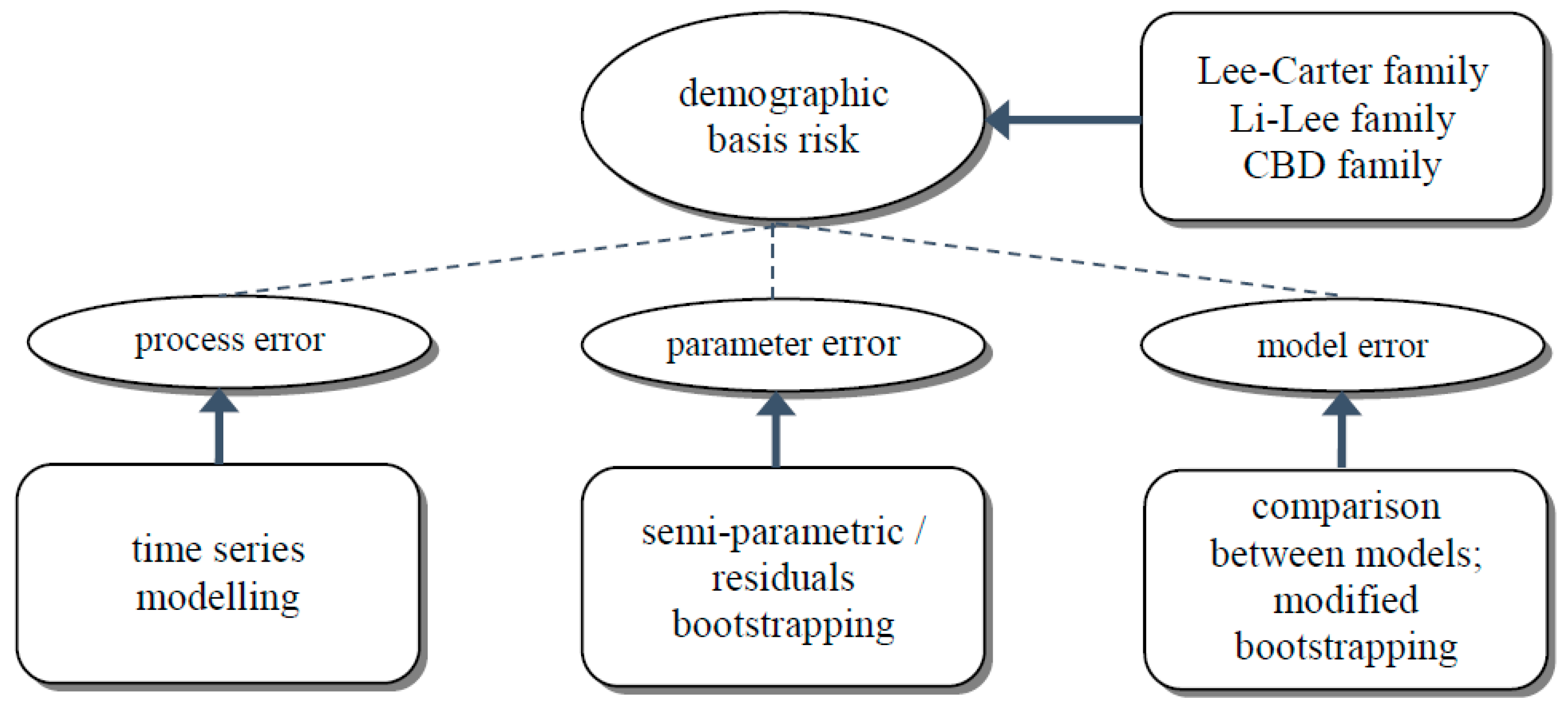
Apart from measuring the hedge effectiveness by testing various models and investigating different simulated scenarios, we also adopt the modified semi-parametric bootstrapping approach in Yang et al. (2015) and incorporate process error, parameter error, and model error simultaneously. It is effectively an extension of the bootstrapping approach suggested by Brouhns et al. (2005). First, a pseudo-sample of the number of deaths is simulated from the Poisson distribution with the observed number of deaths as the mean. Suppose there are two or more competing model candidates under consideration. Each model in turn is fitted to the pseudo-data sample and the corresponding model parameters are estimated. Based on some pre-determined model selection criteria, the most “optimal” model is selected for this particular pseudo-data sample. The time series of the selected model’s temporal parameters are then simulated into the future. Lastly, future death rates are produced from the estimated and simulated parameters of the selected model. So far in this process, the pseudo-data sample is used for generating only one future scenario via one selected model. The entire process above can then be repeated iteratively to create, say, 5000 future scenarios in total1, in which different models may be chosen in different scenarios. In this way, all the three errors are embedded in the simulated future death rates. This modified bootstrapping approach provides a different perspective to understand the impact of model uncertainty, though we acknowledge that the simulation time can be significantly lengthened, especially when more competing models and selection criteria are included in the process. Again, the bootstrapping process needs to be properly adapted to the two-population models. Figure 2 below gives a list of the modeling techniques we experiment with to tackle the different error components. In the next section, we will discuss in detail the similarities and differences between the results on some hypothetical hedging scenarios generated by all these modeling and simulation methods.

3. Hedge Effectiveness

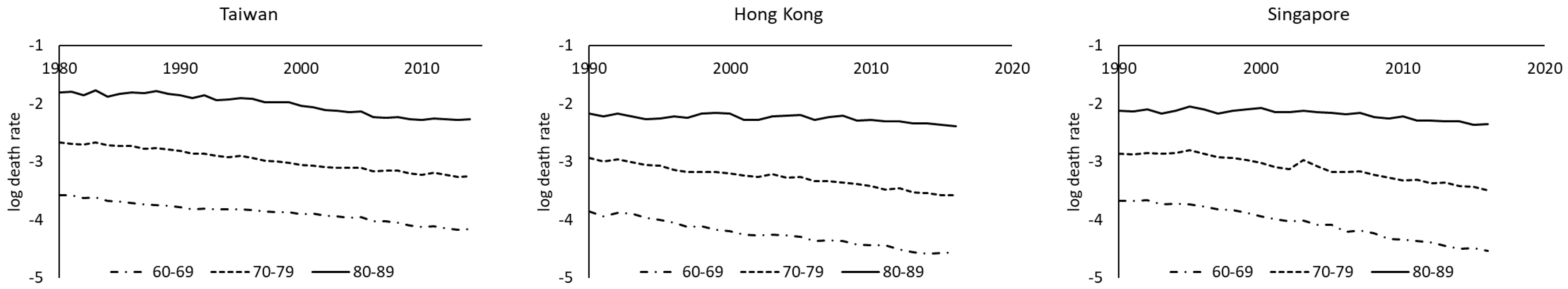
We have collected two sets of data for the book and reference populations. The first set is composed of the male assured lives and pensioners data (book) from the Continuous Mortality Investigation (CMI), and England and Wales male data (reference) from the Human Mortality Database (HMD 2017), for the period from 1983 to 2006. The second set comprises Australia, New Zealand, Japan, Taiwan, Hong Kong (Census and Statistics Department 2017), and Singapore (Department of Statistics 2017) male data from the HMD and governmental statistics departments, for the years 1980 to 2016. Since Asia–Pacific insured data are scarce, we use the data of New Zealand, Taiwan, and Singapore, with relatively smaller sizes, as a proxy for the book population, and the data of their larger neighbors for the reference population. The age range considered is from 60 to 89. Figure 3 plots the log central death rates of three age groups over time. It can be seen that the mortality declining trends of different populations or regions are roughly in line with one another in the past few decades. In general, the death rates of the assured lives and pensioners are lower than those of English and Wales. One potential problem of the assured lives and pensioners data is that there may have been different contributors to the data over the period and there would then be some extent of heterogeneity or inconsistency. Judging simply from the graphs below, it seems that the issue may not be overly significant. Australian death rates are slightly lower than New Zealand death rates, and Japan has experienced lower mortality levels than Taiwan. Hong Kong has had lower mortality experience than Singapore, while the latter is catching up fairly quickly in the last decade.

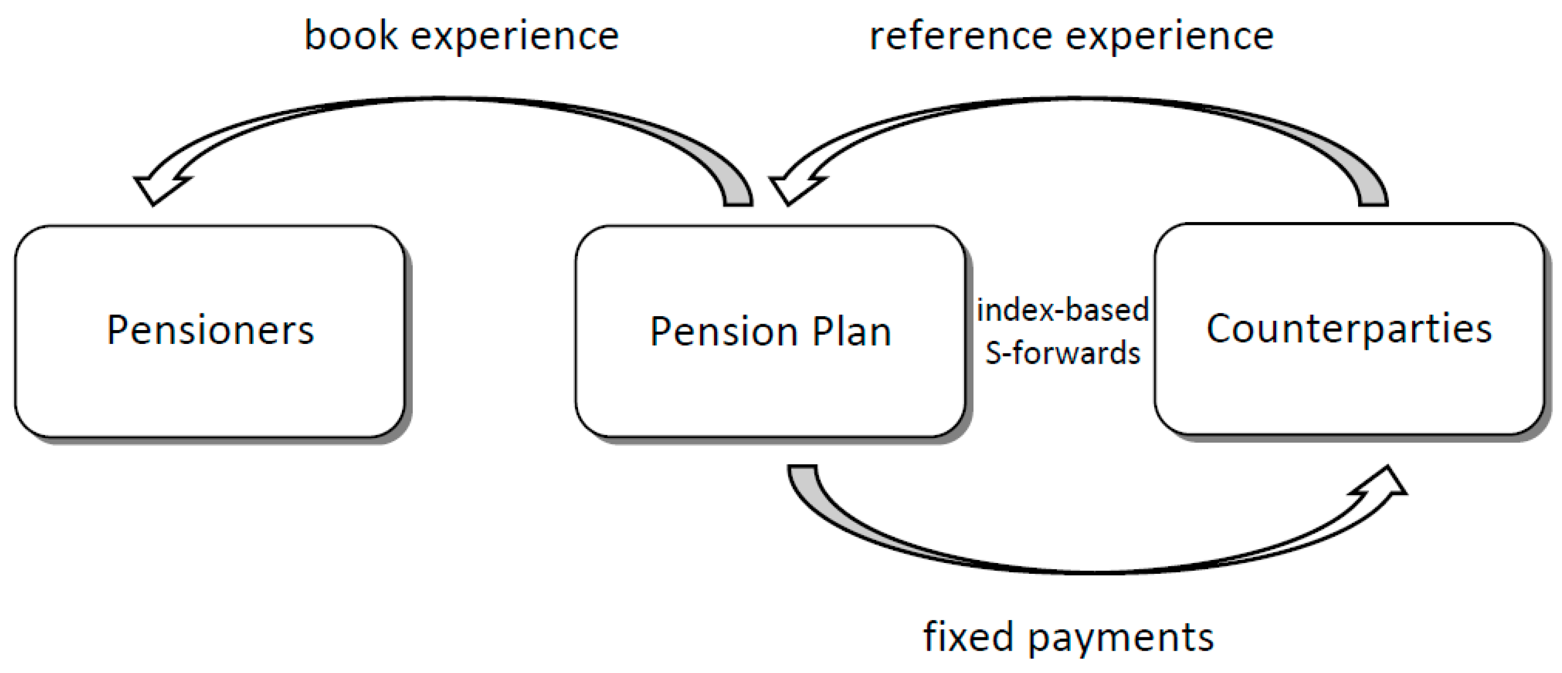
We mainly consider a hypothetical situation of a large pension plan with 10,000 members for a particular cohort. All the pensioners are aged 65 and every pensioner receives $1 on survival of each year in the next 25 years. Suppose that the pension plan financier attempts to minimize its longevity risk exposure by building a longevity hedge with index-based S-forwards (e.g., LLMA 2010), and that the S-forward at every future age is available for the same birth cohort as the pensioners. For a floating rate receiver, the payoff on maturity of a S-forward is equal to the actual survivor index (observed on maturity) minus the forward survivor index (set at time 0), in which the survivor index is the percentage of the reference population who are still alive on maturity. Assume that the current forward values are equal to the central estimates, setting a zero risk premium for convenience, and that the interest rate is constant at 1% p.a. throughout the period, considering the current low interest rate environment. The valuation date is taken as just after the end of the data period.

After fitting the above-mentioned models to the data and carrying out the simulations as in the previous section, we use the simulated future death rates of the book population and the binomial distribution to further simulate the number of surviving pensioners in each future year (e.g., Haberman et al. 2014). We can then obtain random samples of the present value of the pension plan liability. On the other hand, we use the simulated future death rates of the reference population to determine the random S-forwards payoffs, which are discounted to the valuation date. The notional amounts of the S-forwards are calculated by numerical optimization in order to maximize the level of hedge effectiveness (e.g., Li et al. 2017). The weights are mostly in the range of 0.6 to 1.1 (per person) in different cases of our analysis. Figure 4 demonstrates the longevity hedging scheme based on the use of index-based S-forwards. Please note that the counterparties can be a financial exchange or intermediary that brings the market investors (hedge providers) and the pension plan (hedger) into conducting standardized transactions.

Table 1. BIC values of fitting three two-population mortality projection models to different datasets.

Family of Mortality Models	Assured Lives vs. E&W	Pensioners vs. E&W	NZ vs. AUS	TAI vs. JPN	SG vs. HK
Lee–Carter	16,948	16,972	21,577	26,895	4189
Li-Lee	17,049	17,067	21,694	26,897	4207
CBD	16,312	16,376	21,240	29,125	4524

Note: E&W, NZ, AUS, TAI, JPN, SG, and HK represent England and Wales, New Zealand, Australia, Taiwan, Japan, Singapore, and Hong Kong.

lists the BIC (Bayesian Information Criterion) values of fitting the three two-population mortality projection models to the various datasets via an iterative updating scheme based on Newton’s method. In the mortality forecasting literature, the BIC is much more popular than the Akaike Information Criterion (AIC), as it is generally perceived that the BIC imposes a higher penalty on the use of parameters and can point to more parsimonious models. For the first three hedging scenarios, the M7-M5 model (3) produces the lowest BIC values (the italic figures). For the Taiwan pension plan hedged by a Japan index, and also the Singapore pension plan hedged by a Hong Kong index, the bivariate Lee–Carter model (1) gives the lowest BIC, followed very closely by the common factor model (2). Although the BIC is probably the most frequently used selection criterion in the mortality projection modeling literature, it is fundamentally a measure on how good the past patterns are being captured under parsimonious use of parameters, which may or may not lead to accurate or reasonable future predictions. Moreover, as noted earlier, there is always some level of uncertainty in model selection, and the BIC alone (and even together with residuals examination) may point to a less appropriate model given the random fluctuations in the data and the lack of information on possible outliers. In fact, several other model aspects should also be considered (e.g., Cairns et al. 2009). In terms of allowing for longevity basis risk, the most relevant model aspects would be the coherence property, behavior of simulated future variability, and simulation method.

Table 2. Major characteristics of time series processes under different mortality projection models.

Model Choice	Temporal Parameters	Time Series Process	Central Estimates	Variability
(1a) non-coherent	${\mathit{\kappa }}_{t,1},{\mathit{\kappa }}_{t,2}$	BRWD	linear trends	increasing
(1b) non-coherent	${\mathit{\kappa }}_{t,1},{\mathit{\kappa }}_{t,2}$	co-integrated	linear trends	increasing
(1c) non-coherent	${\mathit{\kappa }}_{t,1},{\mathit{\kappa }}_{t,2}$	VECM(p)	long-term linear trends	increasing
(1d) non-coherent	${\mathit{\kappa }}_{t,1},{\mathit{\kappa }}_{t,2}$	VARIMA(p,1,0)	long-term linear trends	increasing
(2)	${\mathit{\kappa }}_t^c$	RWD	linear trend	increasing
(2a) coherent	${\mathit{\kappa }}_{t,1,j},{\mathit{\kappa }}_{t,2,j}$	AR(1)	convergence	bounded
(2b) coherent	${\mathit{\kappa }}_{t,1,j},{\mathit{\kappa }}_{t,2,j}$	AR(p)	convergence	bounded
(2c) coherent	${\mathit{\kappa }}_{t,1,j},{\mathit{\kappa }}_{t,2,j}$	correlated AR(p)	convergence	bounded
(2d) coherent	${\mathit{\kappa }}_{t,1,j},{\mathit{\kappa }}_{t,2,j}$	VAR(p)	convergence	bounded
(3a) coherent	${\mathit{\kappa }}_{t,1}^R,{\mathit{\kappa }}_{t,2}^R,{\mathit{\kappa }}_{t,3}^R$	MRWD	linear trends	increasing
	${\mathit{\kappa }}_{t,1}^B,{\mathit{\kappa }}_{t,2}^B$	VAR(p)	convergence	bounded
(3b) coherent	${\mathit{\kappa }}_{t,1}^R,{\mathit{\kappa }}_{t,2}^R,{\mathit{\kappa }}_{t,3}^R$	VARIMA(p,1,0)	long-term linear trends	increasing
	${\mathit{\kappa }}_{t,1}^B,{\mathit{\kappa }}_{t,2}^B$	VAR(p)	convergence	bounded
(3c) coherent	${\mathit{\kappa }}_{t,1}^R,{\mathit{\kappa }}_{t,2}^R,{\mathit{\kappa }}_{t,3}^R$	MRWD	linear trends	increasing
	${\mathit{\kappa }}_{t,1}^B,{\mathit{\kappa }}_{t,2}^B$	BRW	flat trends	increasing
(3d) coherent	${\mathit{\kappa }}_{t,1}^R,{\mathit{\kappa }}_{t,2}^R,{\mathit{\kappa }}_{t,3}^R$	correlated MRWD	linear trends	increasing
	${\mathit{\kappa }}_{t,1}^B,{\mathit{\kappa }}_{t,2}^B$	& VAR(p)	convergence	bounded

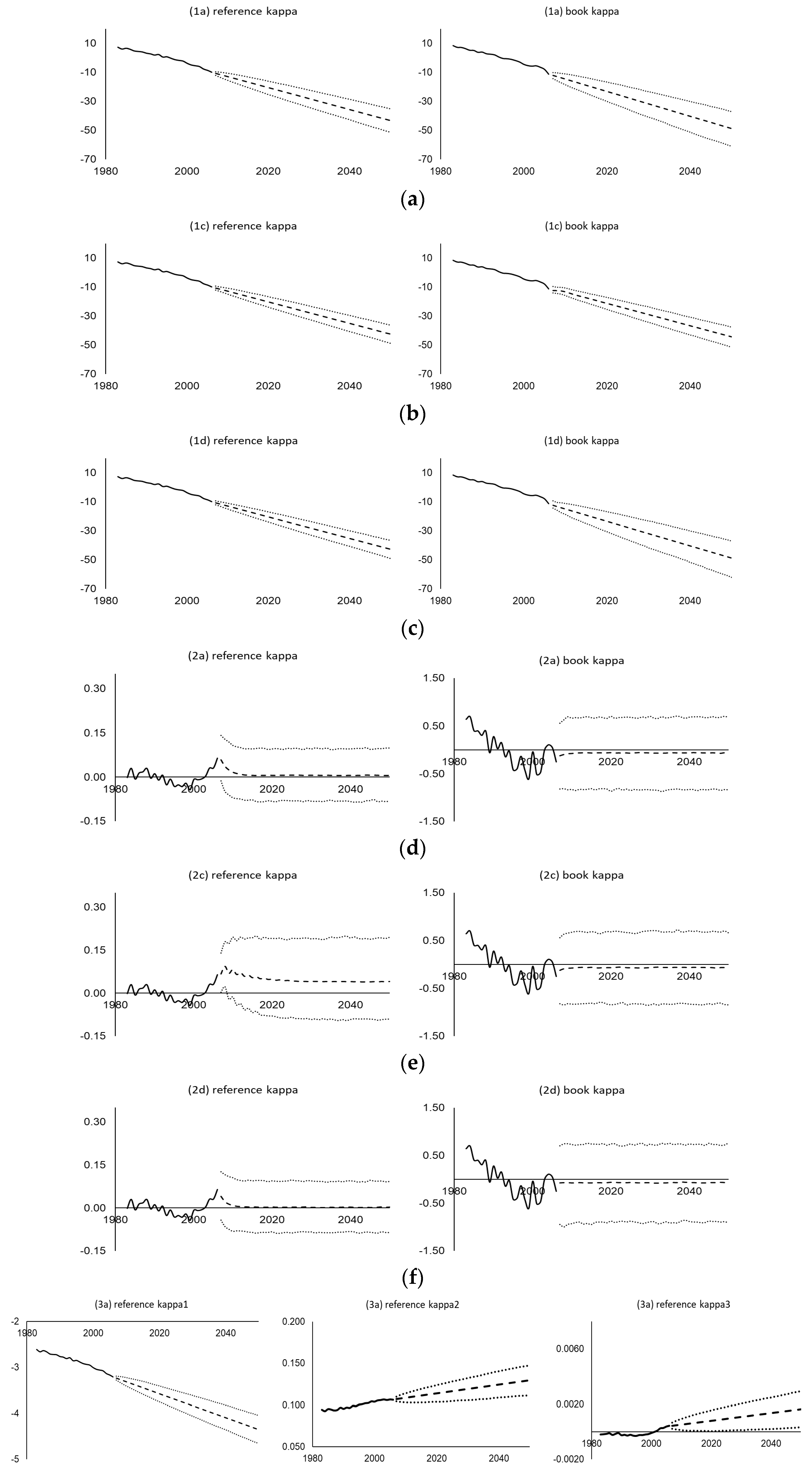
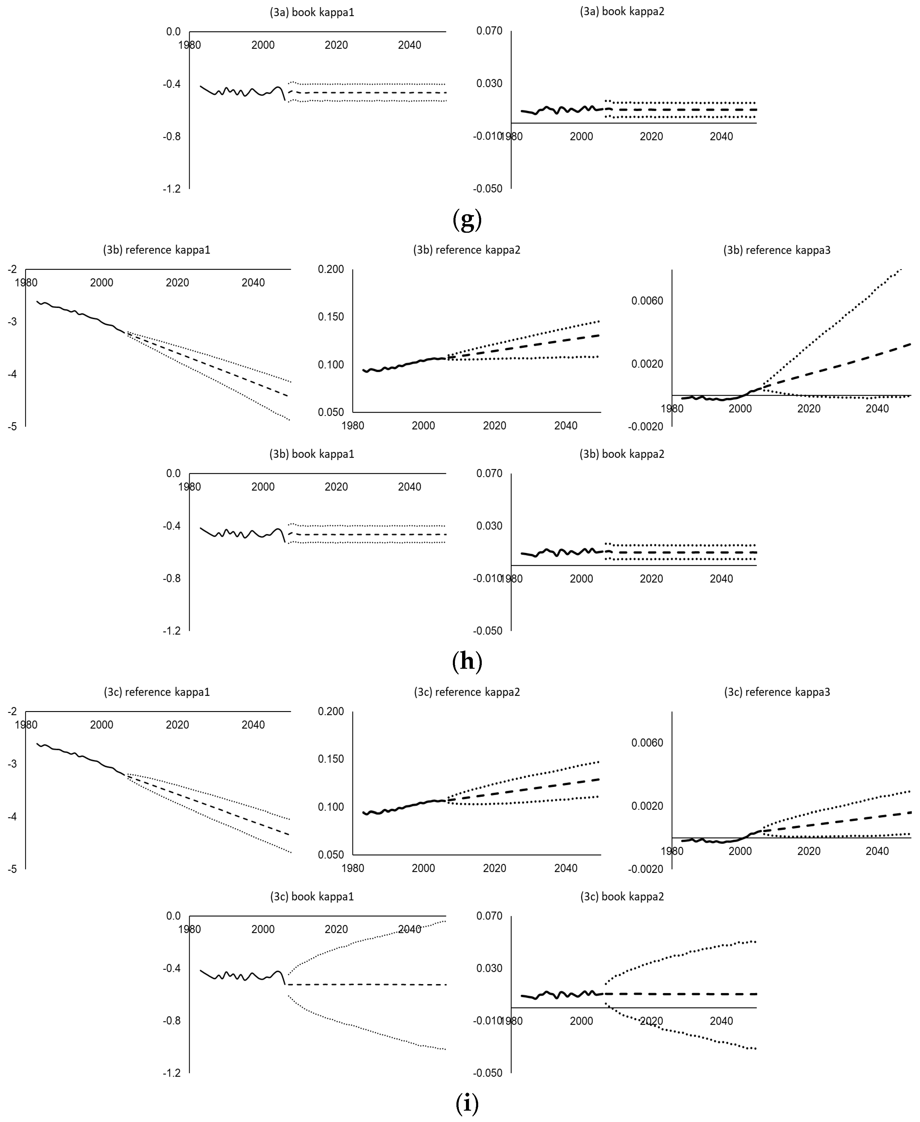
Note: The terms RWD, BRWD, MRWD, and BRW stand for the random walk with drift, bivariate random walk with drift, multivariate random walk with drift, and bivariate random walk without drift, respectively.

summarizes the behavior of the central estimates and simulated variability of each time series process considered.

Table 3. Selected orders of fitted time series processes under different mortality projection models for different datasets.

		Selected Time Series Process
Model Choice	Temporal Parameters	Assured Lives vs. E&W	Pensioners vs. E&W	NZ vs. AUS	TAI vs. JAP	SG vs. HK
(1c)	${\mathit{\kappa }}_{t,1},{\mathit{\kappa }}_{t,2}$	VECM(2)	VECM(2)	VECM(2)	VECM(2)	VECM(2)
(1d)	${\mathit{\kappa }}_{t,1},{\mathit{\kappa }}_{t,2}$	VARIMA(1,1,0)	VARIMA(1,1,0)	VARIMA(1,1,0)	VARIMA(2,1,0)	VARIMA(2,1,0)
(2b)	${\mathit{\kappa }}_{t,1,j},{\mathit{\kappa }}_{t,2,j}$	AR(3), AR(1)	AR(2), AR(3)	AR(2), AR(1)	AR(3), AR(1)/AR(2), AR(1)	AR(1), AR(1)
(2c)	${\mathit{\kappa }}_{t,1,j},{\mathit{\kappa }}_{t,2,j}$	AR(3), AR(1)	AR(2), AR(3)	AR(2), AR(1)	AR(3), AR(1)/AR(2), AR(1)	AR(1), AR(1)
(2d)	${\mathit{\kappa }}_{t,1,j},{\mathit{\kappa }}_{t,2,j}$	VAR(1)	VAR(1)	VAR(2)	VAR(1)/VAR(1)	VAR(1)
(3a)	${\mathit{\kappa }}_{t,1}^B,{\mathit{\kappa }}_{t,2}^B$	VAR(2)	VAR(1)	VAR(1)	VAR(1)	VAR(1)
(3b)	${\mathit{\kappa }}_{t,1}^R,{\mathit{\kappa }}_{t,2}^R,{\mathit{\kappa }}_{t,3}^R$	VARIMA(2,1,0)	VARIMA(2,1,0)	VARIMA(1,1,0)	VARIMA(1,1,0)	VARIMA(1,1,0)
(3b)	${\mathit{\kappa }}_{t,1}^B,{\mathit{\kappa }}_{t,2}^B$	VAR(2)	VAR(1)	VAR(1)	VAR(1)	VAR(1)
(3d)	${\mathit{\kappa }}_{t,1}^B,{\mathit{\kappa }}_{t,2}^B$	VAR(2)	VAR(1)	VAR(1)	VAR(1)	VAR(1)

Note: The selected orders of the fitted time series processes are based on the partial autocorrelation functions and matrices, whether the autocorrelations and cross-correlations of the residuals are insignificant, the estimated parameters are significant, and the resulting fitted time series process (2b, 2c, 2d, 3a, 3b, 3d) is weakly stationary. The weak stationarity can be tested via examining whether all the roots/eigenvalues of the characteristic equation fall inside the unit circle. It can be also tested simply by projecting with the fitted time series process over a long period of time to see whether the projected values converge to a constant. For the Taiwan pension plan hedged by a Japan index, there are two additional factors in the common factor model, while for all the other hedging scenarios, there is only one additional factor. The number of additional factors is based on the lowest BIC value.

provides the details of the selected orders of the fitted time series processes for all the datasets. Figure 5 then shows the various time-varying parameters estimated (solid lines), their central estimate projections (dashed lines), and their simulated 95% prediction intervals (dotted lines) using the UK assured lives data under different mortality projection models and time series processes. As shown, the random walk, co-integrated, VECM, and integrated autoregressive processes all produce linear projected (central estimate) trends and increasing variability across time in the simulations, whereas the (weakly stationary) autoregressive processes show convergence and bounded variability. The widths of the prediction intervals vary between different time series processes. For example, within the Lee–Carter family, the VECM(2) generates narrower intervals for both ${\mathit{\kappa }}_{t,1}$ and ${\mathit{\kappa }}_{t,2}$, and the VARIMA(1,1,0) produces wider intervals for ${\mathit{\kappa }}_{t,2}$ but narrower intervals for ${\mathit{\kappa }}_{t,1}$. For the Li-Lee family, the AR(3) yields wider (bounded) intervals for ${\mathit{\kappa }}_{t,1,1}$ compared to the AR(1) and VAR(1). For the CBD family, the VARIMA(2,1,0) leads to wider intervals for ${\mathit{\kappa }}_{t,1}^R$, ${\mathit{\kappa }}_{t,2}^R$, and ${\mathit{\kappa }}_{t,3}^R$ compared to the multivariate random walk with drift, and the bivariate random walk without drift leads to unbounded intervals for ${\mathit{\kappa }}_{t,1}^B$ and ${\mathit{\kappa }}_{t,2}^B$, in contrast to the bounded intervals from the VAR(2). Some goodness-of-fit test results of the fitted time series processes are given in the Appendix A.

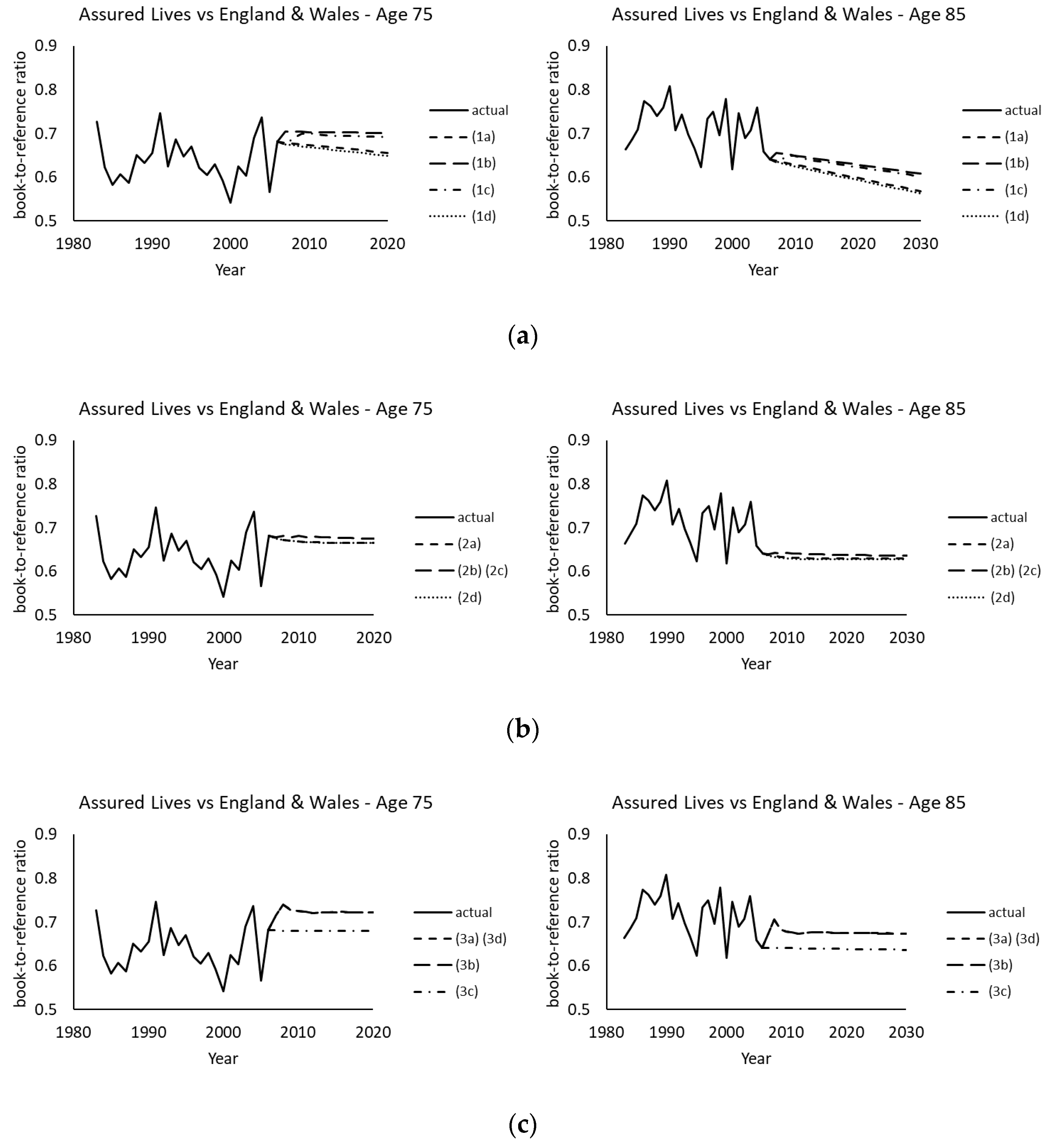
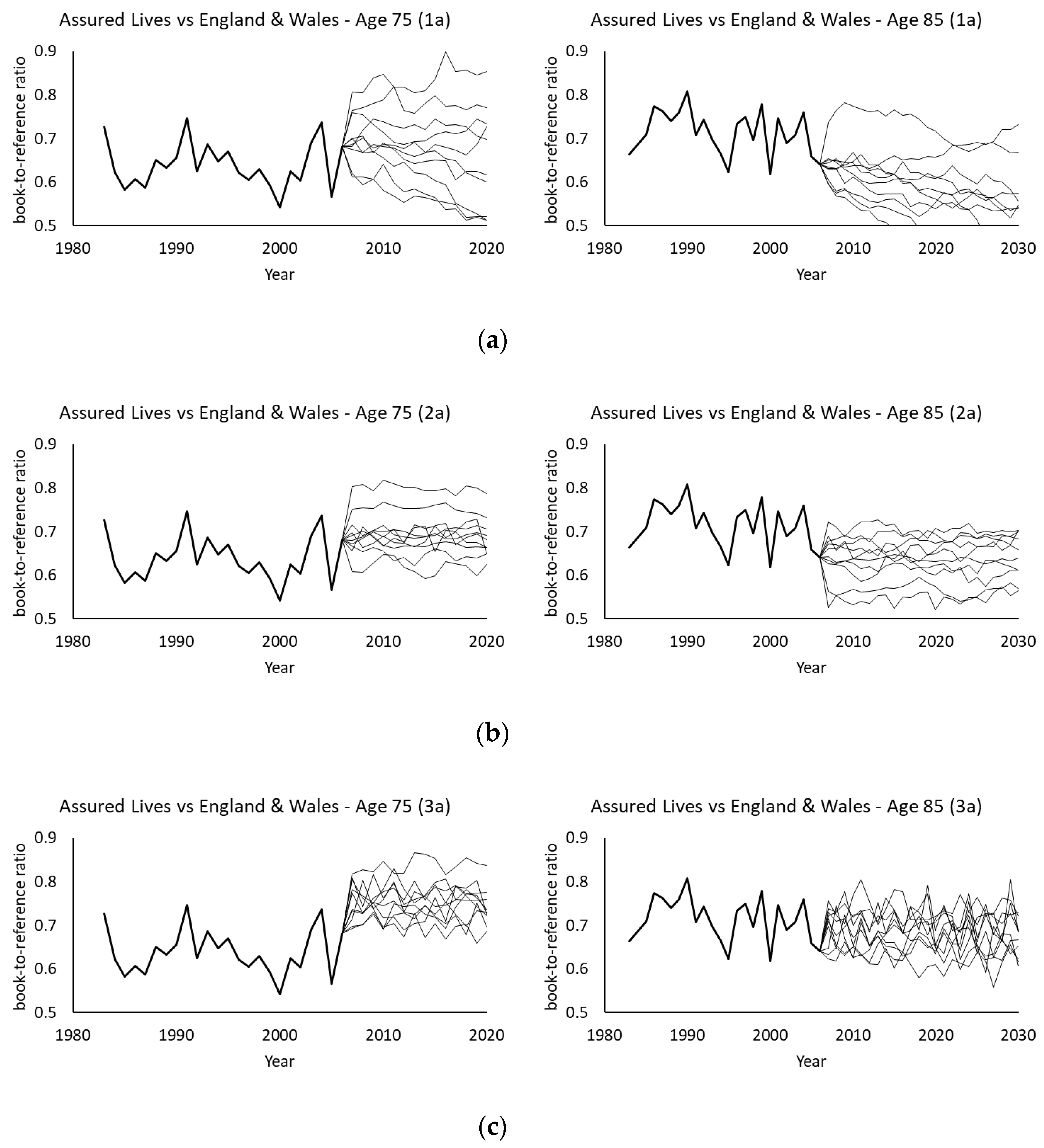
Figure 6 plots the corresponding book-to-reference ratios of projected death rates at ages 75 and 85. In agreement with the descriptions in the previous section, models (1a) to (1d) produce divergent ratios of projected death rates between the two populations. Moreover, the projected ratios diverge in various directions at different ages even under the same model. By contrast, models (2a) to (2d) and (3a) to (3d) yield convergent ratios of projected death rates at each age, which are in the range of around 0.6 to 0.7 as illustrated in the plots. Figure 7 then displays some simulated ratios using 10 randomly picked simulated paths. There are clear differences between model (1a) and models (2a) and (3a). Under model (1a), the simulated ratios can move to values very different from the projected ones over time, while under models (2a) and (3a), the simulated ratios fluctuate around the projected levels. The potential variations under model (1a) are much greater than those under models (2a) and (3a), in which model (3a) demonstrates more obvious fluctuations but within a shorter distance from the projected values than model (2a). Since demographic basis risk arises from possible deviations between the book and reference mortality movements (due to demographic or socioeconomic differences), the behavior of these simulated ratios of death rates would have a significant implication on the calculated levels of hedge effectiveness, which will be discussed in the following numerical analysis.

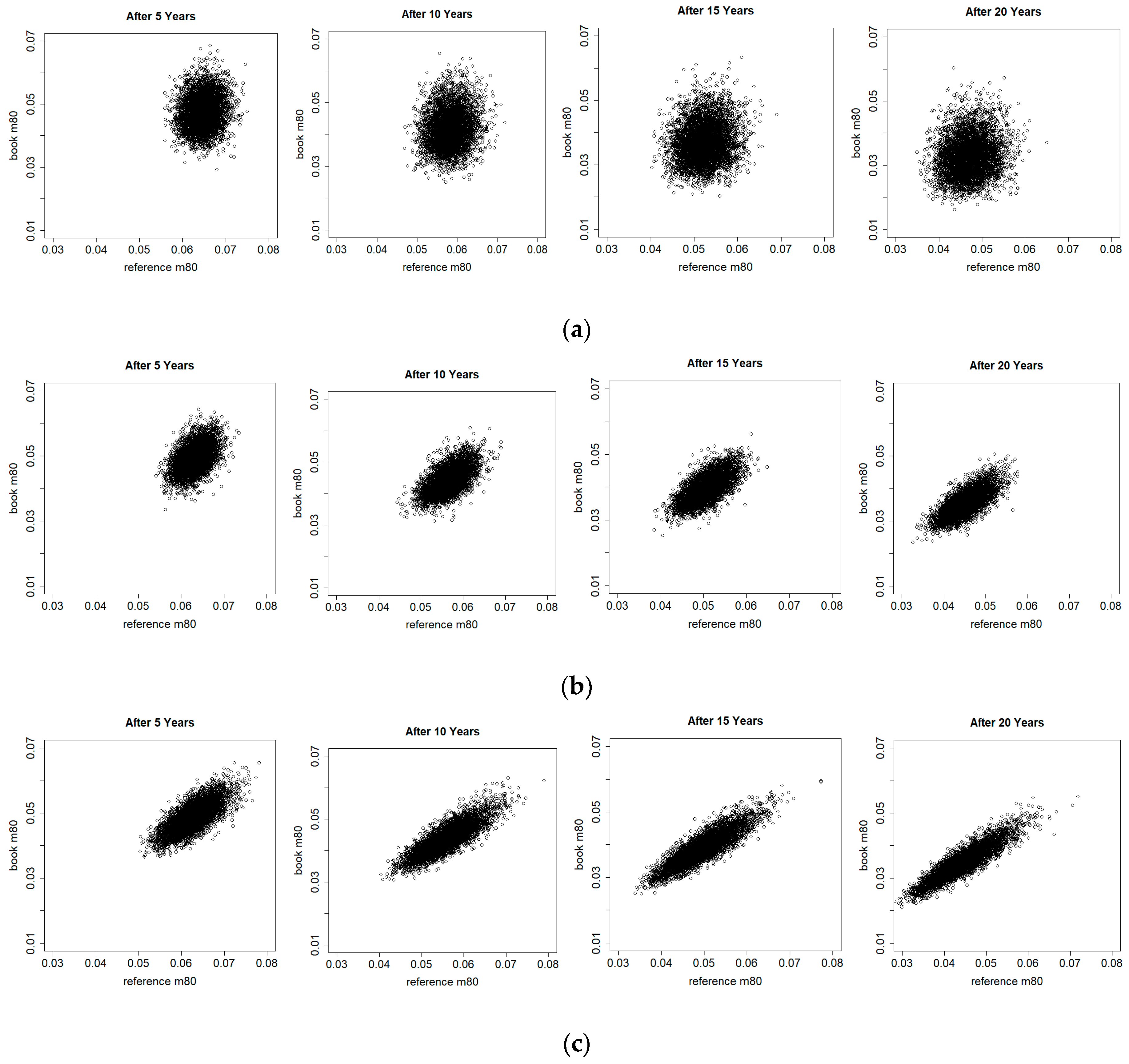
Figure 8 offers a different view on the simulated book and reference death rates at age 80 at different points of time using the UK pensioners data. It can be seen that over time, the simulated death rates move to the southwest direction due to mortality improvements, and the simulated variability (both the vertical and horizontal ranges) increases because of higher uncertainty in more distant future. However, again, there are significant differences between the three models. For models (2a) and (3a), the dependence between the simulated book and reference death rates increases gradually with time, whereas for model (1a), the weak dependence appears to remain at a low level. It means that for the former the two death rates are very unlikely to deviate significantly further from each other in the long term, but for the latter the two death rates can move in varying directions. The different model structures clearly have a large impact on the resulting association between the two populations in the simulations. The discussion of the numerical study below will explore the underlying reasons for these observations. These simulated differences in the dependence would affect the calculation of basis risk and hedge effectiveness significantly, as shown later.

Table 4. Standard deviation and 99.5% VaR (minus mean) of pension plan liability (in % of mean).

Model Choice	Assured Lives	Pensioners	NZ	TAI	SG
	Monte Carlo simulation
SD
(1a)/(1b)/(1c)/(1d)	1.3/1.1/0.9/1.4	2.3/1.5/1.1/1.6	1.8/1.5/1.1/1.3	1.9/1.7/1.1/0.9	1.7/2.0/1.1/1.1
(2a)/(2b)/(2c)/(2d)	1.1/1.1/1.1/1.1	1.4/1.3/1.4/1.4	1.4/1.4/1.4/1.4	1.7/1.7/1.7/1.7	1.6/1.6/1.7/1.6
(3a)/(3b)/(3c)/(3d)	1.6/1.6/2.5/1.6	1.9/1.8/3.1/1.7	2.0/1.4/3.2/2.0	1.9/1.4/2.6/1.8	2.5/1.7/3.4/2.2
VaR
(1a)/(1b)/(1c)/(1d)	3.1/1.1/0.9/1.4	5.6/3.8/2.7/3.9	4.5/3.6/2.8/3.4	4.6/4.4/2.8/2.3	4.2/4.8/2.7/2.7
(2a)/(2b)/(2c)/(2d)	2.6/2.7/2.7/2.7	3.5/3.3/3.3/3.4	3.5/3.5/3.4/3.4	4.3/4.3/4.3/4.3	3.9/3.9/4.1/3.9
(3a)/(3b)/(3c)/(3d)	3.8/3.9/5.9/3.8	4.6/4.5/7.5/4.3	5.1/3.5/7.5/5.0	4.8/3.6/6.6/4.9	5.2/4.2/7.9/5.5
	Semi-parametric bootstrapping
SD
(1a)/(1b)/(1c)/(1d)	1.5/1.2/0.9/1.5	2.5/1.5/1.1/1.7	2.0/1.6/1.1/1.4	1.9/1.8/1.1/0.9	2.0/2.2/1.2/1.2
(2a)/(2b)/(2c)/(2d)	1.1/1.1/1.1/1.1	1.4/1.4/1.4/1.4	1.5/1.4/1.4/1.5	1.7/1.7/1.7/1.7	1.8/1.8/1.8/1.7
(3a)/(3b)/(3c)/(3d)	1.6/1.5/2.7/1.6	1.9/1.9/3.2/1.7	2.1/1.4/3.4/2.1	1.9/1.5/2.7/1.8	2.7/1.8/3.8/2.5
VaR
(1a)/(1b)/(1c)/(1d)	3.9/2.9/2.5/4.9	5.9/3.8/2.8/4.2	5.4/3.8/2.8/3.5	5.1/4.5/2.9/2.4	4.8/5.2/2.8/3.1
(2a)/(2b)/(2c)/(2d)	2.9/2.8/2.7/2.9	3.6/3.5/3.6/3.4	3.6/3.5/3.6/3.6	4.4/4.2/4.4/4.3	4.3/4.3/4.4/4.2
(3a)/(3b)/(3c)/(3d)	3.9/5.0/6.7/3.7	4.7/6.1/7.7/4.2	5.1/3.6/8.5/5.1	4.7/3.7/6.6/4.6	5.6/4.5/8.6/6.2
	Residuals bootstrapping
SD
(1a)/(1b)/(1c)/(1d)	1.6/1.2/1.0/1.6	2.5/1.5/1.1/1.7	2.0/1.5/1.1/1.4	2.0/1.8/1.1/0.9	2.2/2.6/1.3/1.2
(2a)/(2b)/(2c)/(2d)	1.2/1.2/1.2/1.2	1.4/1.4/1.4/1.4	1.4/1.4/1.4/1.4	1.7/1.7/1.7/1.7	1.9/1.9/1.8/1.9
(3a)/(3b)/(3c)/(3d)	1.6/1.5/2.9/1.6	1.9/1.9/3.4/1.8	2.1/1.4/3.4/2.1	1.9/1.4/2.8/1.8	2.9/1.9/4.2/2.6
VaR
(1a)/(1b)/(1c)/(1d)	4.1/3.0/2.5/5.5	6.0/3.7/2.8/4.5	5.0/3.7/2.9/3.8	4.8/4.8/3.0/2.4	5.3/5.8/3.1/3.1
(2a)/(2b)/(2c)/(2d)	3.0/2.9/3.1/2.9	3.5/3.6/3.5/3.5	3.6/3.6/3.6/3.6	4.3/4.6/4.3/4.3	4.6/4.6/4.6/4.5
(3a)/(3b)/(3c)/(3d)	3.9/4.3/6.7/3.8	4.7/5.8/8.0/4.5	5.2/3.5/8.4/5.1	5.0/3.5/7.0/4.8	5.9/4.6/8.9/6.8
	Bivariate residuals bootstrapping
SD
(1a)/(1b)/(1c)/(1d)	1.5/1.2/1.0/1.7	2.5/1.5/1.2/1.7	2.0/1.5/1.1/1.4	2.0/1.9/1.1/1.0	2.2/2.5/1.3/1.2
(2a)/(2b)/(2c)/(2d)	1.2/1.2/1.2/1.2	1.4/1.4/1.5/1.4	1.4/1.4/1.4/1.4	1.8/1.7/1.7/1.7	1.8/1.8/1.9/1.9
(3a)/(3b)/(3c)/(3d)	1.6/1.5/2.8/1.6	1.9/1.9/3.3/1.8	2.1/1.4/3.5/2.1	2.0/1.4/2.8/1.8	2.9/1.8/4.2/2.7
VaR
(1a)/(1b)/(1c)/(1d)	4.1/3.1/2.5/5.3	6.2/3.8/3.0/4.5	5.1/3.7/2.8/3.6	5.2/4.6/2.9/2.3	5.4/5.9/3.1/3.1
(2a)/(2b)/(2c)/(2d)	2.9/2.9/3.1/3.1	3.5/3.7/3.6/3.6	3.4/3.4/3.5/3.5	4.4/4.4/4.5/4.3	4.4/4.4/4.6/4.5
(3a)/(3b)/(3c)/(3d)	3.9/4.6/6.8/4.1	4.9/5.8/8.0/4.4	5.2/3.6/8.1/4.9	5.0/3.6/6.8/4.7	6.1/4.7/8.9/6.5
	Modified semi-parametric bootstrapping
SD
(1b) + (2a) + (3a)	1.6	1.9	2.1	1.8	2.0
VaR
(1b) + (2a) + (3a)	4.0	4.8	5.0	4.5	5.1

sets out the estimates of the standard deviation and the 99.5% Value-at-Risk (VaR) (minus the mean) of the present value of the pension plan liability, as a percentage of the expected present value of the liability. On average, the standard deviation is about 1.7% and the 99.5% VaR is around 4.3% of the mean, in which the ratio between the two measures is close to that of a standard normal distribution. For the assured lives and pensioners datasets, the bootstrapping approaches generally give larger VaR estimates than those from Monte Carlo simulation (the cells within borders), while for the other datasets, the differences are less obvious. The potential heterogeneity issue of the former may be the reason they demonstrate a greater effect of parameter uncertainty. The simulated variability from the Li-Lee family (2a, 2b, 2c, 2d) (the shaded rows), but not the other two families, is fairly robust to the selection of time series process. Model (3c) produces by far the largest estimates (the bolded figures) among all the models. It appears that the bivariate random walk for ${\mathrm{K}}_t^B$ together with the multivariate random walk for ${\mathrm{K}}_t^R$ in model (3c) produces much more variability in the book simulations compared with the other models.

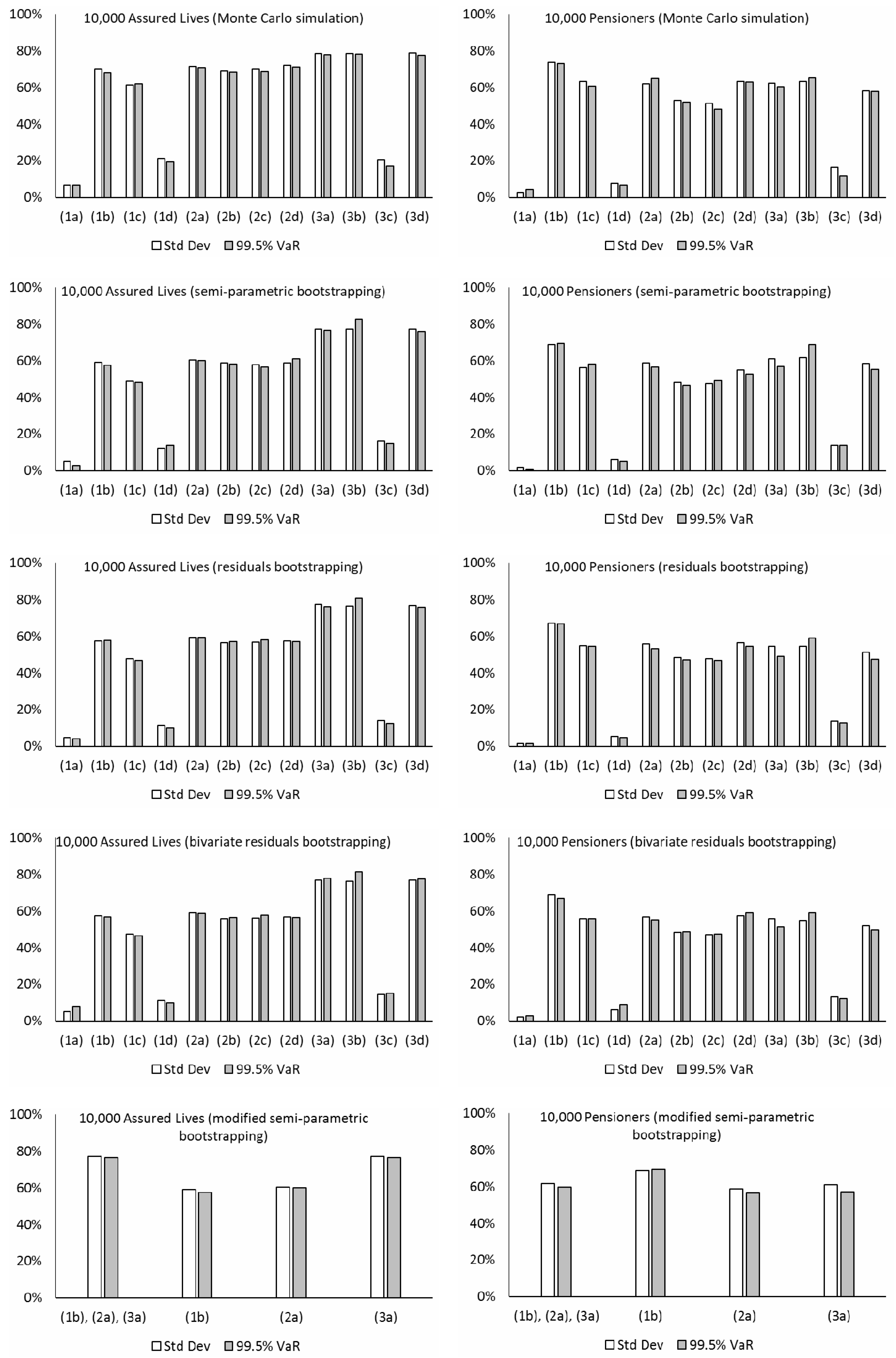
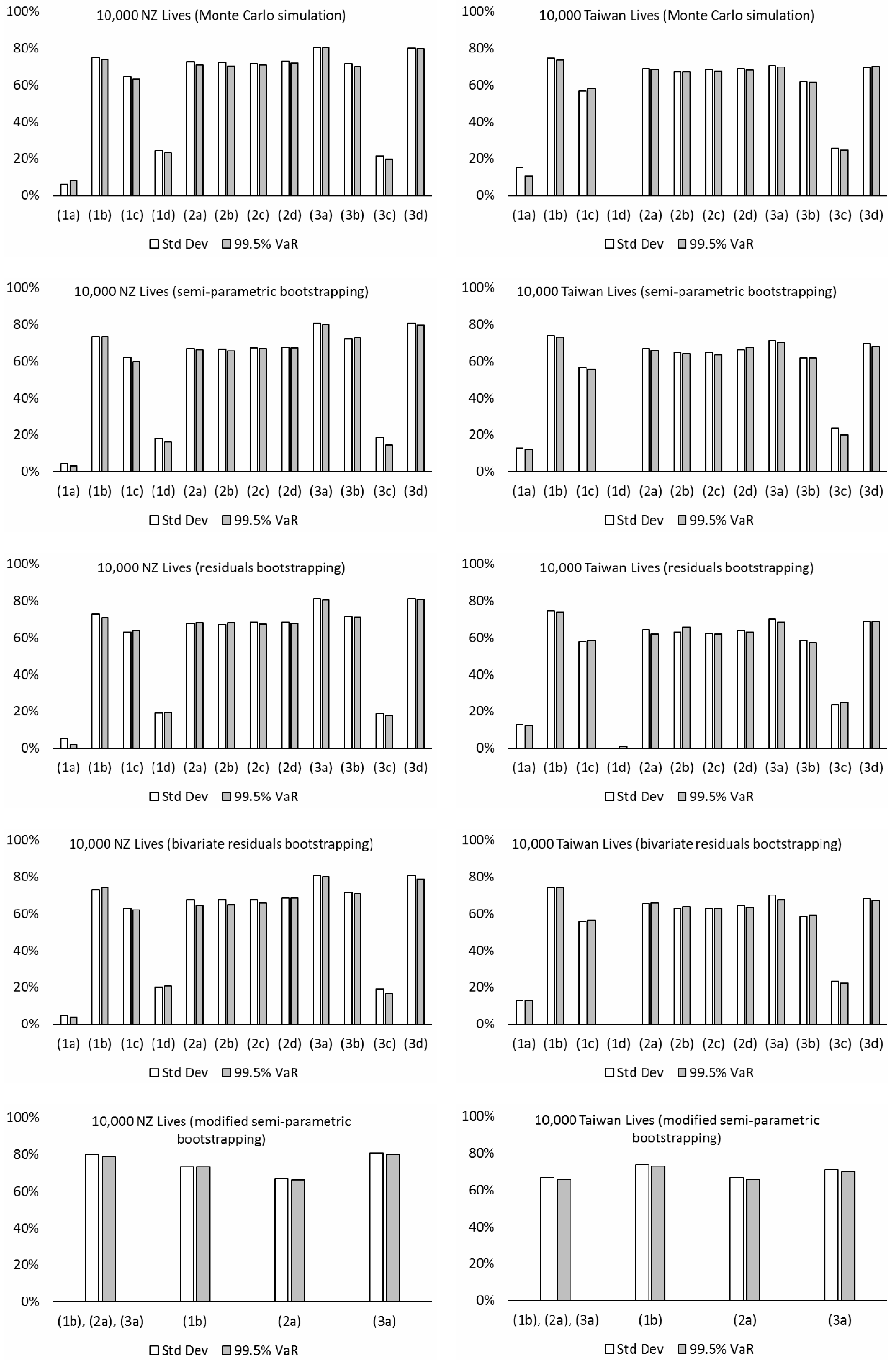
In line with Coughlan et al. (2011) and Li et al. (2017), the level of hedge effectiveness is defined as [1 – risk_hedged/risk_unhedged] × 100%. The two quantities risk_unhedged and risk_hedged are the pension plan’s longevity risk exposure before and after implementing the hedge. This measure gives the proportion of the original longevity risk exposure that is being transferred away. The remaining risk can then be seen as a result of longevity basis risk. We consider the longevity risk exposure as the standard deviation and the 99.5% VaR minus the mean of the present value of the pension plan liability. Please note that the 99.5% VaR measure is highly relevant to the Solvency Capital Requirement (SCR) calculation under Solvency II. It is a very important consideration for insurance practitioners and regulators in Europe. Figure 9 presents the levels of hedge effectiveness (i.e., the proportion of the initial risk that is reduced) under various models and simulation methods using different datasets. The major observations and implications from the numerical results are listed below:

• The estimated levels of hedge effectiveness are largely between 50% to 80%. The clear exceptions include those produced from models (1a), (1d), and (3c), which are about 20% or lower. The first two of these three cases are non-coherent and generate increasing variability in the time-varying parameters’ future simulations for both the book and reference populations. Although the estimated correlations in their Gaussian error terms are quite high (about 0.3 or greater), the relationship between the book and reference mortality levels under the two models looks too weak, when considering their past movements in the data (see Figure 3), and there is an overestimation of longevity basis risk. Comparatively, while models (1b) and (1c) are also non-coherent, their co-integration and error correction structures lead to some extent of co-movements between the two populations in the simulations, which is reflected in the estimated hedge effectiveness. The last exception, model (3c), is coherent, but it produces increasing simulated variability over time for the “book minus reference” component’s time-varying parameters. The resulting effect is that the simulated book and reference mortality movements could deviate significantly from each other, progressively so over the long run, leading to an overestimation of longevity basis risk and so an underestimation of hedge effectiveness. By contrast, the other model choices do not suffer from this problem.
• The results from the Li-Lee family (2a, 2b, 2c, 2d) are generally quite robust to the choice of time series modeling, as long as the fitted time series processes are weakly stationary. Under the Li-Lee mortality structure, both populations are governed by the common factor, in which the common mortality index has increasing variability over time in the simulations, while the additional population-specific factors’ time-varying parameters have bounded variability in the simulations under all the four choices. Consequently, the former variability would dominate eventually, and any deviance between the simulated book and reference mortality movements is unlikely to continue to grow. The figures from models (2b) and (2c) are slightly lower than those from model (2a) (by only about 3% in magnitude on average; more obvious for the pensioners dataset), due to the higher selected orders in the former. However, in general there is not much difference in the results between models (2b) and (2c), and also between models (2a) and (2d), which suggest that the additional dependence (via correlation or vector autoregression) is unlikely to have a material impact on assessing longevity basis risk. Besides, though the common factor provides a convenient way to capture the link between the two populations, the common factor model (2) requires using the same data length for both populations in maximum likelihood estimation. In practice, the length of book data is usually shorter, and approximation methods or Bayesian techniques may be adopted to fit the model under the presence of missing data.
• The figures from models (3a), (3b), and (3d) of the CBD family tend to be higher than those from models (2a) and (2d) (by about 10% in magnitude or more) for the assured lives and the New Zealand portfolios, while the two sets of results differ more randomly for the other datasets. Under these models, the reference component’s temporal parameters have increasing simulated variability over time, while the “book minus reference” component’s temporal parameters have bounded simulated variability instead. The variability in the reference component would then dominate in the long term, whereas the variability in the second component would become less influential comparatively. The consequence is that the book and reference mortality movements cannot deviate indefinitely in the simulated scenarios. The results are about the same between models (3a) and (3d), which again suggest that the additional dependence (via correlation) does not have an obvious effect on measuring longevity basis risk. For model (3b), as noted previously, the prediction intervals for ${\mathit{\kappa }}_{t,1}^R$, ${\mathit{\kappa }}_{t,2}^R$, and ${\mathit{\kappa }}_{t,3}^R$ based on the VARIMA process are often different to those based on the multivariate random walk with drift in model (3a). Some subsequent effect can be seen in the differences between the figures from models (3a) and (3b), in which the latter ones tend to be lower.
• The hedging results estimated from Monte Carlo simulation tend to be higher than those from the bootstrapping approaches (by about 7% in magnitude on average) for the assured lives and pensioners datasets. Since performing Monte Carlo simulation directly on the error terms of the time series processes allows for only process error but not parameter error, there would be an underestimation of longevity basis risk and hence an overestimation of hedge effectiveness. But for the other datasets (New Zealand, Taiwan, and Singapore), there are no such obvious differences, which indicate that the effect of parameter uncertainty is not material for these proxy book data with a large size and more stable population compositions and mortality patterns. In addition, there are no clear, significant differences between the results estimated from the two residuals bootstrapping approaches, in which one involves resampling the reference and book residuals separately and the other groups together the two sets of residuals in each age-time cell as an individual data point for resampling. It means that the additional dependence from linking the residuals does not appear to have any effect on longevity basis risk calculation. Some random differences in the results between the semi-parametric bootstrapping and the residuals bootstrapping can also be seen, but most of them are small and do not show any particular patterns.
• For a demonstration of applying the modified semi-parametric bootstrapping approach, we integrate models (1b), (2a), and (3a) which have earlier been shown to produce more reasonable estimates of hedge effectiveness. Following Yang et al. (2015), the optimal model for each pseudo-data sample in the bootstrapping process is selected based on the BIC. That is, the BIC values of fitting the three mortality projection models are compared, and the one with the lowest value is chosen for that pseudo-data. Note that besides a single statistical criterion, a mix of other quantitative and even qualitative criteria may also be used, though the selection rules will then be more complex, and the computation time will lengthen.

  Table 5. Simulated proportions of model selections in modified semi-parametric bootstrapping for different datasets.

  	Simulated Proportions of Model Selections
  Model Choice	Assured Lives vs. E&W	Pensioners vs. E&W	NZ vs. AUS	TAI vs. JAP	SG vs. HK
  (1b)	0%	0%	0%	1%	42%
  (2a)	0%	0%	0%	99%	58%
  (3a)	100%	100%	100%	0%	0%

  gives the proportions of different models being chosen out of 5000 scenarios in each case. For the assured lives, pensioners, and New Zealand datasets, model (3a) dominates in all the simulated scenarios. For the Taiwan portfolio, model (2a) is selected in 99% of the scenarios and model (1b) is selected in only 1%. For the Singapore portfolio, models (2a) and (1b) share a split of 58% and 42%. Furthermore, as shown in Figure 9 (last row), regarding the Singapore portfolio, the final hedging results from this approach may be perceived as a “weighted” average of those calculated separately from models (1b) and (2a), in which the “weights” are determined by how well the two models are fitted to each of the 5000 pseudo-data samples.
• The estimated levels of hedge effectiveness are quite close between using the standard deviation and 99.5% VaR in most cases. This observation may result from the fact that the simulated distributions of the pension plan liability are fairly symmetric and do not have a heavy tail, under all the mortality projection models, time series processes, and simulation methods considered, both before and after hedging. We have also checked the results based on the 95% VaR and the observations are similar.
• When the size of the pension plan is reduced to 1000 members, the levels of hedge effectiveness estimated from those coherent models drop to mostly around 20% to 40% (not shown here). By contrast, when the pension plan size is infinite (i.e., the step of using the binomial distribution to simulate the number of lives is omitted), the estimated levels of hedge effectiveness largely rise by about 10% or more in magnitude from the initial setting of 10,000 members. The effect of sampling basis risk is significant, which pinpoints that index-based longevity hedging would be more feasible for either very large pension plans, foundations joined by small pension plans, or reinsurers who have accumulated sizable longevity risk exposures from smaller insurers and pension plans.
• There are some differences in the hedging results between using the five datasets. On average, after integrating both process error and parameter error via the bootstrapping approaches, the highest level of hedge effectiveness is given by using the New Zealand dataset, followed by the Taiwan, assured lives, Singapore, and pensioners datasets. It has been mentioned earlier that parameter error would be immaterial for book data with stable population compositions and mortality patterns, which may explain some of the results here. Another possible reason for the greater hedge effectiveness shown by the New Zealand pension plan hedged by an Australia index is the geographical and cultural closeness between Australia and New Zealand. Both neighbors are island nations in the South Pacific and have very close connections historically, socially, and economically, and they would tend to have more concurrent mortality movements than otherwise.
• Under models (2a), (2b), (2c), (2d), (3a), (3b), and (3d), the calculated levels of hedge effectiveness of the annual cash flows (not the present value; not shown here) are indeed very low in the early years, but then increase significantly across time, i.e., the dependence between the two populations’ mortality levels grows with time in the simulations. For the Li-Lee model types, the common mortality index has increasing variability, while the additional time-varying parameters have bounded variability. Similarly, for the M7-M5 model types, the reference component’s time-varying parameters have increasing variability, but the book component’s time-varying parameters have bounded variability. The resulting model effect is that the simulated variability of the differences between both populations would have lesser impact gradually. Hence the association between the two populations increases over time (see Figure 8).
• The weights of the S-forwards are numerically optimized to maximize the hedge effectiveness. Excluding models (1a), (1d), and (3c) which generate unreasonable simulations, for the assured lives dataset, the weights are roughly about 0.5 (per person) in the first half of the age range, 0.7 in the third quarter, and 0.9 in the last quarter. For the pensioners dataset, the weights are around 0.7 in the first half of the age range and 0.9 in the second half. For the New Zealand, Taiwan, and Singapore datasets, most of the weights are approximately equal to one for the whole range. Interestingly, the major patterns in the weights estimated are not too different between the various models. It should be noted that these weights are subject to the technical limitations of the optimization process, uncertainty of the model choice, and random variations in the simulated samples. In addition, in practice, it would be impossible to enter into such numerically precise amounts of S-forward positions due to liquidity issues. Accordingly, we have also tested the hedging results using the approximate weights noted above, and we realize that the corresponding reductions in the levels of hedge effectiveness are actually quite small, mostly being a few percent in magnitude.

4. Concluding Remarks

In this paper, we study the impact of model uncertainty on hedging longevity risk via index-based derivatives and measuring longevity basis risk. We adopt three families of mortality projection models, using several time series processes and simulation methods, to calibrate index-based S-forwards, construct longevity hedges, and assess the resulting hedge effectiveness. Notably, we test various combinations of mortality models and time series processes different to those in the existing literature and examine their impact in detail. Overall, the estimated levels of hedge effectiveness are mostly about 50% to 80% for a large pension plan, which is in line with those in Li et al. (2017) using different models and datasets to those adopted here, but the precise levels still depend heavily on the selected model. In particular, while the choice of mortality models has certain effects, it appears that the selection of time series processes has a far greater impact on the index-based hedging results. Unfortunately, the length of the assured lives and pensioners data available is short, and application of more sophisticated time series processes cannot be further investigated. Apart from comparing the results from different models, the semi-parametric bootstrapping approach can also be extended to include selection criteria and test several models simultaneously. However, those models or time series processes with unrestricted simulated variability in the differences between the book and reference populations lead to irrational hedging results and should be avoided. In practice, the final model choice relies not only on a quantitative analysis of (usually limited) past book data but also on some extent of qualitative judgement about uncertain future mortality trends and the user’s own knowledge or preference.

There are a few possible areas for future research. So far, we focus on static hedging, under which the hedging tools are not rebalanced in the future. By contrast, dynamic hedging requires constant rebalancing of the hedged portfolio, and it would be interesting to explore the feasibility of dynamic index-based longevity hedging. For simplicity, we also assume that the forward rates are equal to the central estimates, implying a zero premium on longevity risk. To further incorporate the costs of longevity hedging, it would be useful to investigate different risk-neutral methods (e.g., Cairns et al. 2006) for pricing index-based derivatives. Moreover, Li et al. (2017) considered some simple model extensions to take structural mortality changes and mortality jumps into account when assessing the hedge effectiveness. More sophisticated methods such as regime-switching models (e.g., Milidonis et al. 2011) and copulas (e.g., Wang et al. 2015) can further be tested in modeling these extreme events. In addition, we use a single information criterion in the modified semi-parametric bootstrapping process. Alternatively, a more complex set of rules consisting of multiple quantitative and qualitative criteria may provide a more realistic view of model uncertainty. Lastly, Bayesian techniques can also be adopted to allow for model uncertainty directly, instead of using the modified bootstrapping approach above. For instance, two or more competing models can be integrated into the Bayesian framework by setting a prior distribution for all the model candidates (e.g., Cairns 2000).

References

- Brouhns, Natacha, Michel Denuit, and Ingrid Van Keilegom. 2005. Bootstrapping the Poisson log-bilinear model for mortality forecasting. Scandinavian Actuarial Journal 2005: 212–24. [Google Scholar] [CrossRef]
- Cairns, Andrew J. G. 2000. A discussion of parameter and model uncertainty in insurance. Insurance: Mathematics and Economics 27: 313–30. [Google Scholar] [CrossRef] [Green Version]
- Cairns, Andrew J. G. 2013. Robust hedging of longevity risk. Journal of Risk and Insurance 80: 621–48. [Google Scholar] [CrossRef]
- Cairns, Andrew J. G., David Blake, and Kevin Dowd. 2006. A two-factor model for stochastic mortality with parameter uncertainty: Theory and calibration. Journal of Risk and Insurance 73: 687–718. [Google Scholar] [CrossRef]
- Cairns, Andrew J. G., David Blake, and Kevin Dowd. 2008. Modelling and management of mortality risk: A review. Scandinavian Actuarial Journal 2008: 79–113. [Google Scholar] [CrossRef]
- Cairns, Andrew J. G., David Blake, Kevin Dowd, Guy D. Coughlan, and Marwa Khalaf-Allah. 2011. Bayesian stochastic mortality modelling for two populations. ASTIN Bulletin 41: 29–59. [Google Scholar]
- Cairns, Andrew J. G., David Blake, Kevin Dowd, Guy D. Coughlan, David Epstein, Alen Ong, and Igor Balevich. 2009. A quantitative comparison of stochastic mortality models using data from England and Wales and the United States. North American Actuarial Journal 13: 1–35. [Google Scholar] [CrossRef]
- Carter, Lawrence R., and Ronald D. Lee. 1992. Modeling and forecasting US sex differentials in mortality. International Journal of Forecasting 8: 393–411. [Google Scholar] [CrossRef]
- Census and Statistics Department, Hong Kong Special Administrative Region. 2017. Census and Statistics Department: Hong Kong Special Administrative Region. In Demographic Trends in Hong Kong 1986–2016. Hong Kong: Census and Statistics Department, Hong Kong Special Administrative Region. [Google Scholar]
- Chan, Wai-Sum, Johnny Siu-Hang Li, and Jackie Li. 2014. The CBD mortality indexes: Modeling and applications. North American Actuarial Journal 18: 38–58. [Google Scholar] [CrossRef]
- Committee of European Insurance and Occupational Pensions Supervisors (CEIOPS). 2010. QIS5 Technical Specifications. Available online: https://www.bafin.de/SharedDocs/Downloads/DE/Versicherer_Pensionsfonds/QIS/dl_adapted_technical_specifications.pdf?__blob=publicationFile&v=2 (accessed on 30 July 2020).
- Coughlan, Guy D., Marwa Khalaf-Allah, Yijing Ye, Sumit Kumar, Andrew J. G. Cairns, David Blake, and Kevin Dowd. 2011. Longevity hedging 101: A framework for longevity basis risk analysis and hedge effectiveness. North American Actuarial Journal 15: 150–76. [Google Scholar] [CrossRef] [Green Version]
- Coughlan, Guy, David Epstein, Amit Sinha, and Paul Honig. 2007. q-Forwards: Derivatives for Transferring Longevity and Mortality Risks; Pension Advisory Group, JPMorgan. Available online: https://www.researchgate.net/publication/256109844_q-Forwards_Derivatives_for_Transferring_Longevity_and_Mortality_Risks (accessed on 30 July 2020).
- Cowley, Alex, and J. David Cummins. 2005. Securitization of life insurance assets and liabilities. Journal of Risk and Insurance 72: 193–226. [Google Scholar] [CrossRef]
- Department of Statistics, Ministry of Trade & Industry, Republic of Singapore. 2017. Population Trends 2017. Singapore: Department of Statistics, Ministry of Trade & Industry. [Google Scholar]
- Haberman, Steven, and Arthur Renshaw. 2011. A comparative study of parametric mortality projection models. Insurance: Mathematics and Economics 48: 35–55. [Google Scholar] [CrossRef] [Green Version]
- Haberman, Steven, Vladimir Kaishev, Pietro Millossovich, Andrés Villegas, Steven Baxter, Andrew Gaches, Sveinn Gunnlaugsson, and Mario Sison. 2014. Longevity Basis Risk—A Methodology for Assessing Basis Risk. Institute and Faculty of Actuaries (IFoA), and Life and Longevity Markets Association (LLMA). London: IFoA. [Google Scholar]
- HMD (Human Mortality Database). 2017. University of California, Berkeley (USA) and Max Planck Institute for Demographic Research (Germany). Available online: www.mortality.org (accessed on 18 January 2018).
- Koissi, Marie-Claire, Arnold F. Shapiro, and Goran Högnäs. 2006. Evaluating and extending the Lee-Carter model for mortality forecasting: Bootstrap confidence interval. Insurance: Mathematics and Economics 38: 1–20. [Google Scholar] [CrossRef]
- LCP (Lane Clark & Peacock LLP). 2012. LCP Pension Buy-Ins, Buy-Outs and Longevity Swaps 2012. Available online: https://www.lcp.uk.com/media/458733/lcp%20buy-out%20report%202012.pdf (accessed on 30 July 2020).
- Lee, Ronald D., and Lawrence R. Carter. 1992. Modeling and forecasting U.S. mortality. Journal of the American Statistical Association 87: 659–71. [Google Scholar] [CrossRef]
- Li, Jackie, and Steven Haberman. 2015. On the effectiveness of natural hedging for insurance companies and pension plans. Insurance: Mathematics and Economics 61: 286–97. [Google Scholar] [CrossRef] [Green Version]
- Li, Jackie, Leonie Tickle, Chong It Tan, and Johnny Siu-Hang Li. 2017. Assessing Basis Risk for Longevity Transactions—Phase 2. Macquarie University, Institute and Faculty of Actuaries (IFoA), and Life and Longevity Markets Association (LLMA). London: IFoA. [Google Scholar]
- Li, Jackie, Michel Dacorogna, and Chong It Tan. 2014. The impact of joint mortality modelling on hedging effectiveness of mortality derivatives. Paper presented at Tenth International Longevity Risk and Capital Markets Solutions Conference, Santiago, Chile, September 4. [Google Scholar]
- Li, Jackie. 2013. A Poisson common factor model for projecting mortality and life expectancy jointly for females and males. Population Studies 67: 111–26. [Google Scholar] [CrossRef]
- Li, Jackie. 2014. A quantitative comparison of simulation strategies for mortality projection. Annals of Actuarial Science 8: 281–97. [Google Scholar] [CrossRef]
- Li, Johnny Siu-Hang, and Ancheng Luo. 2012. Key q-duration: A framework for hedging longevity risk. ASTIN Bulletin 42: 413–52. [Google Scholar]
- Li, Johnny Siu-Hang, Wai-Sum Chan, and Rui Zhou. 2016. Semicoherent multipopulation mortality modeling: The impact on longevity risk securitization. Journal of Risk and Insurance 84: 1025–65. [Google Scholar] [CrossRef]
- Li, Nan, and Ronald Lee. 2005. Coherent mortality forecasts for a group of populations: An extension of the Lee-Carter method. Demography 42: 575–94. [Google Scholar] [CrossRef] [Green Version]
- LLMA (Life and Longevity Markets Association). 2010. Technical Note: The S-Forward. Available online: https://www.actuaries.org.uk/system/files/documents/pdf/b1.pdf (accessed on 30 July 2010).
- Milidonis, Andreas, Yijia Lin, and Samuel H. Cox. 2011. Mortality regimes and pricing. North American Actuarial Journal 15: 266–89. [Google Scholar] [CrossRef]
- Ngai, Andrew, and Michael Sherris. 2011. Longevity risk management for life and variable annuities: The effectiveness of static hedging using longevity bonds and derivatives. Insurance: Mathematics and Economics 49: 100–14. [Google Scholar] [CrossRef]
- Plat, Richard. 2009. Stochastic portfolio specific mortality and the quantification of mortality basis risk. Insurance: Mathematics and Economics 45: 123–32. [Google Scholar]
- Tan, Chong It, Jackie Li, Johnny Siu-Hang Li, and Uditha Balasooriya. 2014. Parametric mortality indexes: From index construction to hedging strategies. Insurance: Mathematics and Economics 59: 285–99. [Google Scholar] [CrossRef]
- Tsai, Jeffrey T., Larry Y. Tzeng, and Jennifer L. Wang. 2011. Hedging longevity risk when interest rates are uncertain. North American Actuarial Journal 15: 201–11. [Google Scholar] [CrossRef]
- Tsay, Ruey S. 2002. Analysis of Financial Time Series. New York: John Wiley & Sons. [Google Scholar]
- Wang, Chou-Wen, Sharon S. Yang, and Hong-Chih Huang. 2015. Modeling multi-country mortality dependence and its application in pricing survivor index swaps—A dynamic copula approach. Insurance: Mathematics and Economics 63: 30–39. [Google Scholar] [CrossRef]
- Yang, Bowen, Jackie Li, and Uditha Balasooriya. 2015. Using bootstrapping to incorporate model error for risk-neutral pricing of longevity risk. Insurance: Mathematics and Economics 62: 16–27. [Google Scholar] [CrossRef]
- Yang, Bowen, Jackie Li, and Uditha Balasooriya. 2016. Cohort extensions of the Poisson common factor model for modelling both genders jointly. Scandinavian Actuarial Journal 2016: 93–112. [Google Scholar] [CrossRef]
- Yang, Sharon S., and Chou-Wen Wang. 2013. Pricing and securitization of multi-country longevity risk with mortality dependence. Insurance: Mathematics and Economics 52: 157–69. [Google Scholar] [CrossRef]
- Zhou, Kenneth Q., and Johnny Siu-Hang Li. 2016. Dynamic longevity hedging in the presence of population basis risk: A feasibility analysis from technical and economic perspectives. Journal of Risk and Insurance 84: 417–37. [Google Scholar] [CrossRef]