
Thermo-Economic Analysis of Near-Surface Geothermal Energy Considering Heat and Cold Supply within a Low-Temperature District Heating Network


Abstract
:1. Introduction
- Holistic simulation of the heating network, consumers, and geothermal heat sources using resilient user profiles;
- Investigation of geothermal heat sources with respect to the heating and cooling capacity;
- Evaluation of these heat sources for various scenarios in terms of thermodynamic and economic aspects.
2. Methodology
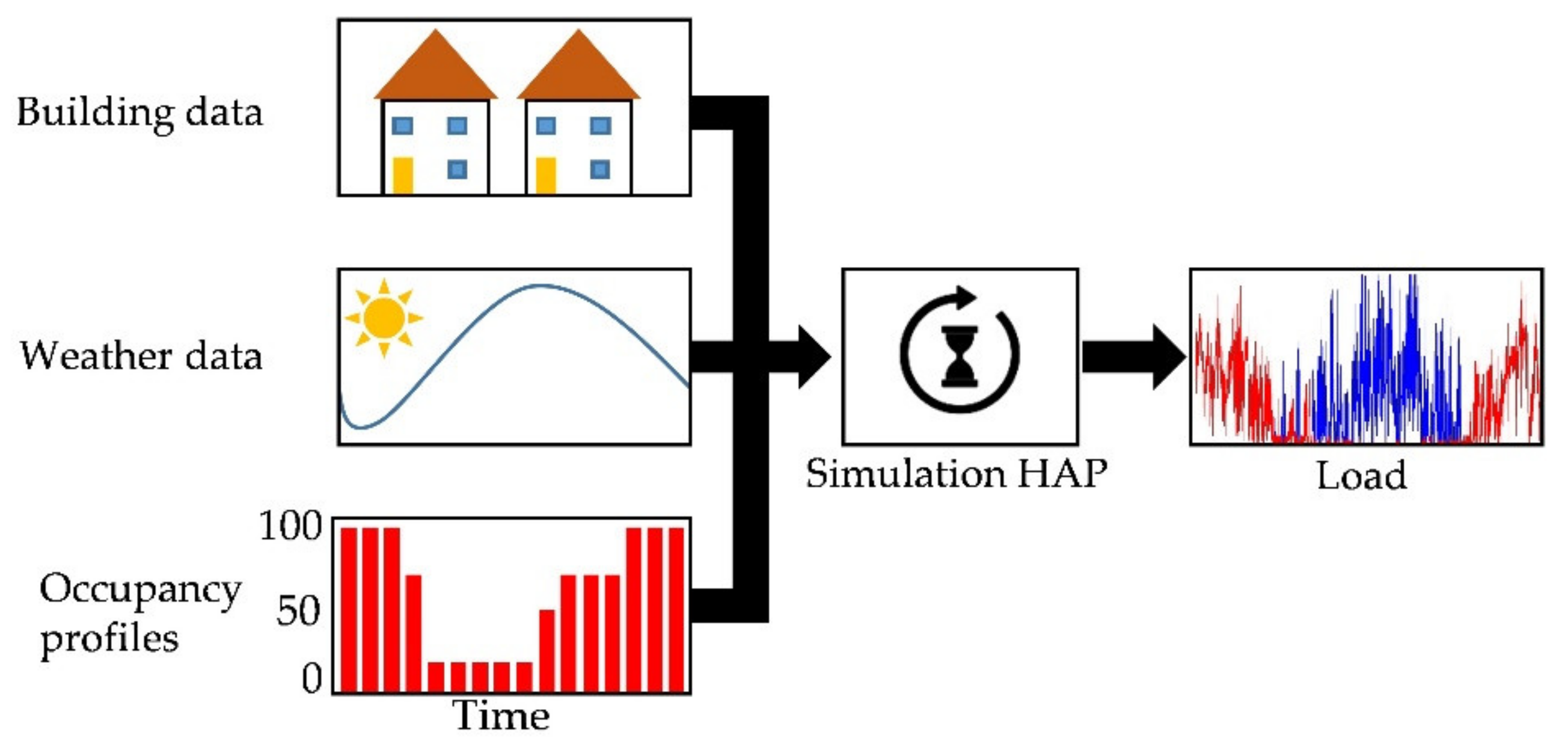
- Location and Weather: The weather data used in this model consist of the dry bulb temperature, which is provided by ASHRAE [13] for the investigated region of Stuttgart. In addition, all parameters that characterise the ground of the considered location, such as density, heat capacity, and thermal conductivity are considered;
- Distance: The distance between users is necessary for the calculation of pressure and heat losses or gains within the pipeline;
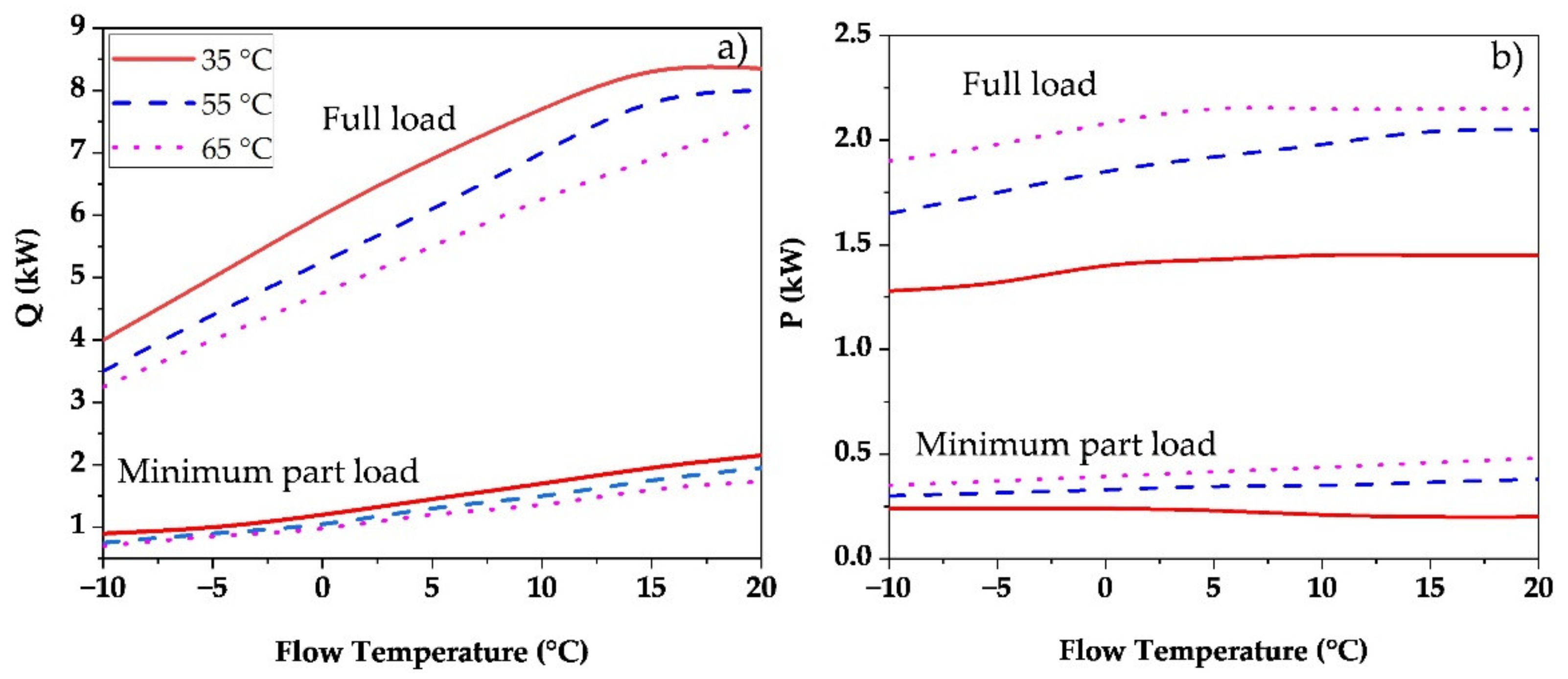
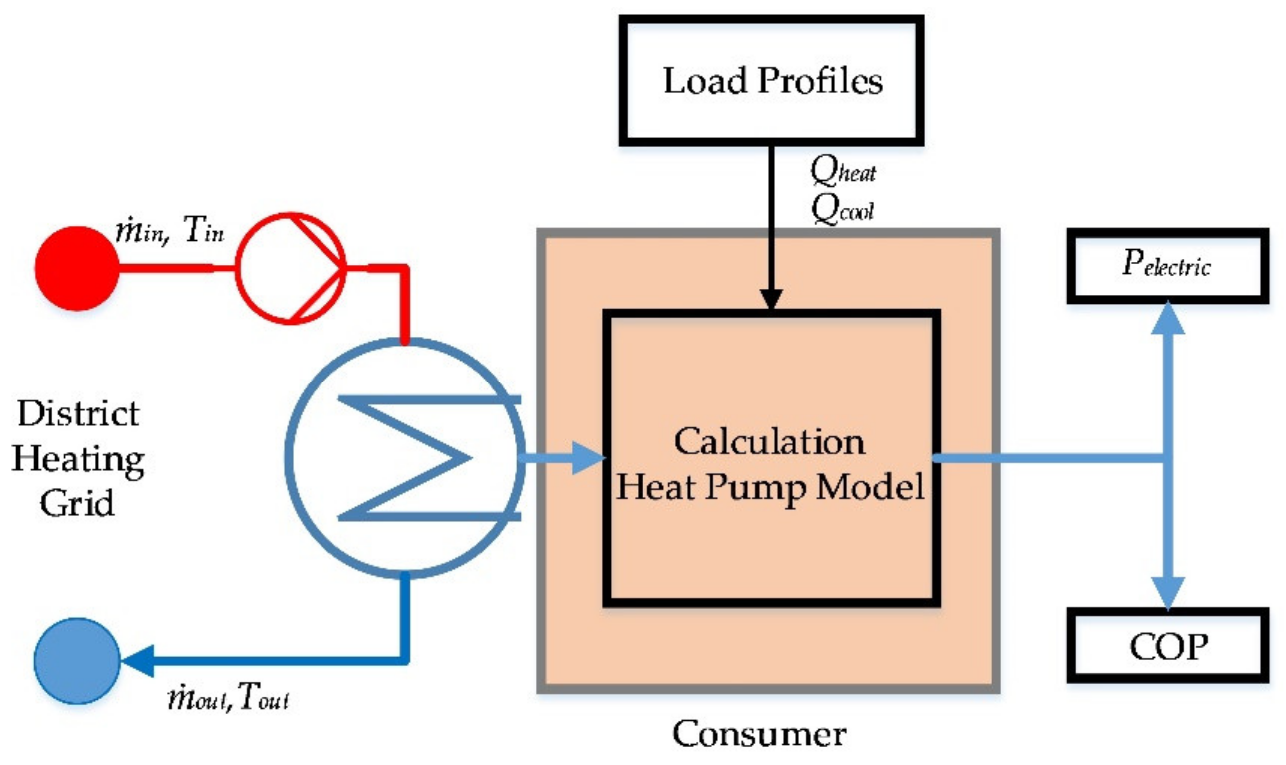
- Consumers: Each user is described by three thermal demand profiles for heating, cooling, and domestic hot water. Furthermore, the characteristic curves of the heat pump for each load case are implemented.
- Global outputs represent the energy balances that concern the entire network, such as total energy imported or exported from the pipeline and the effect on the geothermal heat source.
- Local outputs show the effects on the consumer, such as electrical power consumption of the heat pump and sufficient supply of the load profiles.
2.1. Distribution System
2.2. Consumer
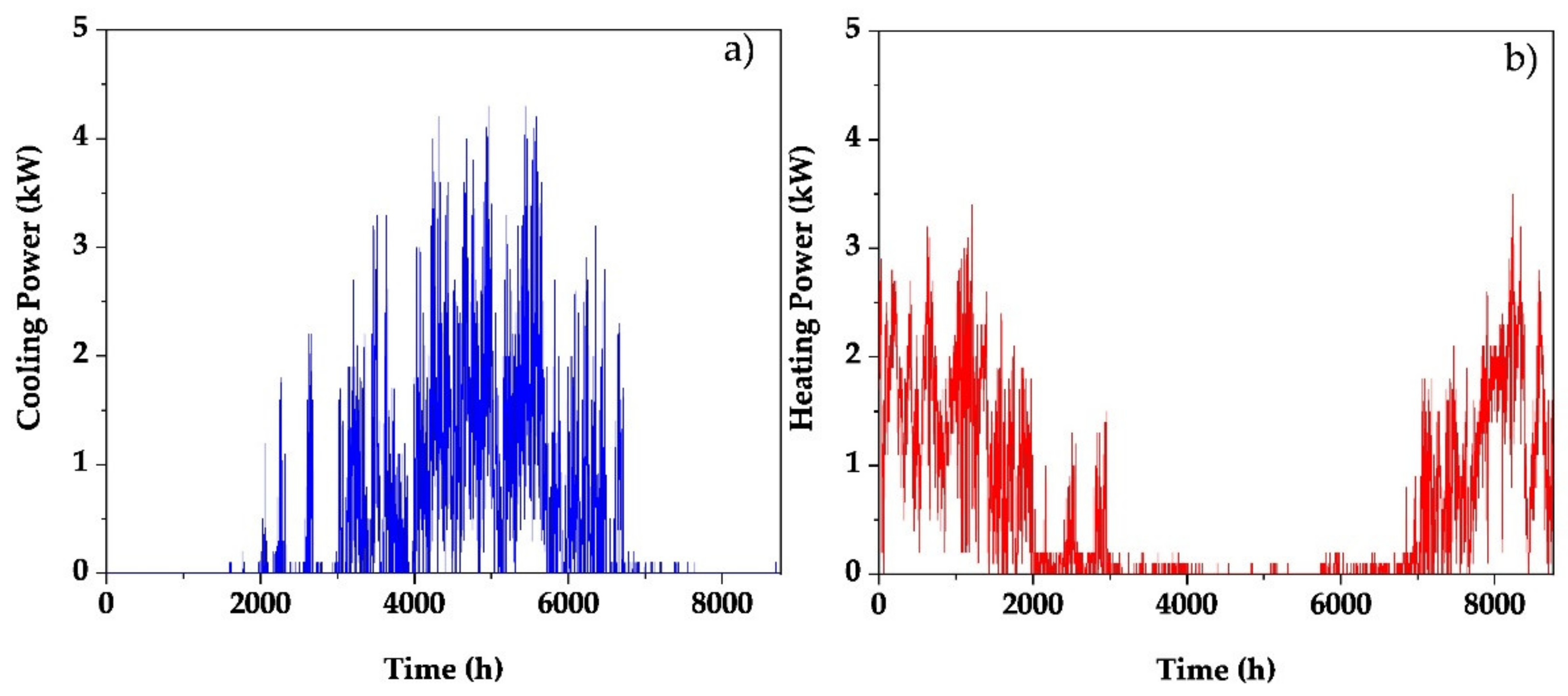
2.3. Load Profiles
2.4. Geothermal Heat Sources
2.5. Economical Assessment
3. Results
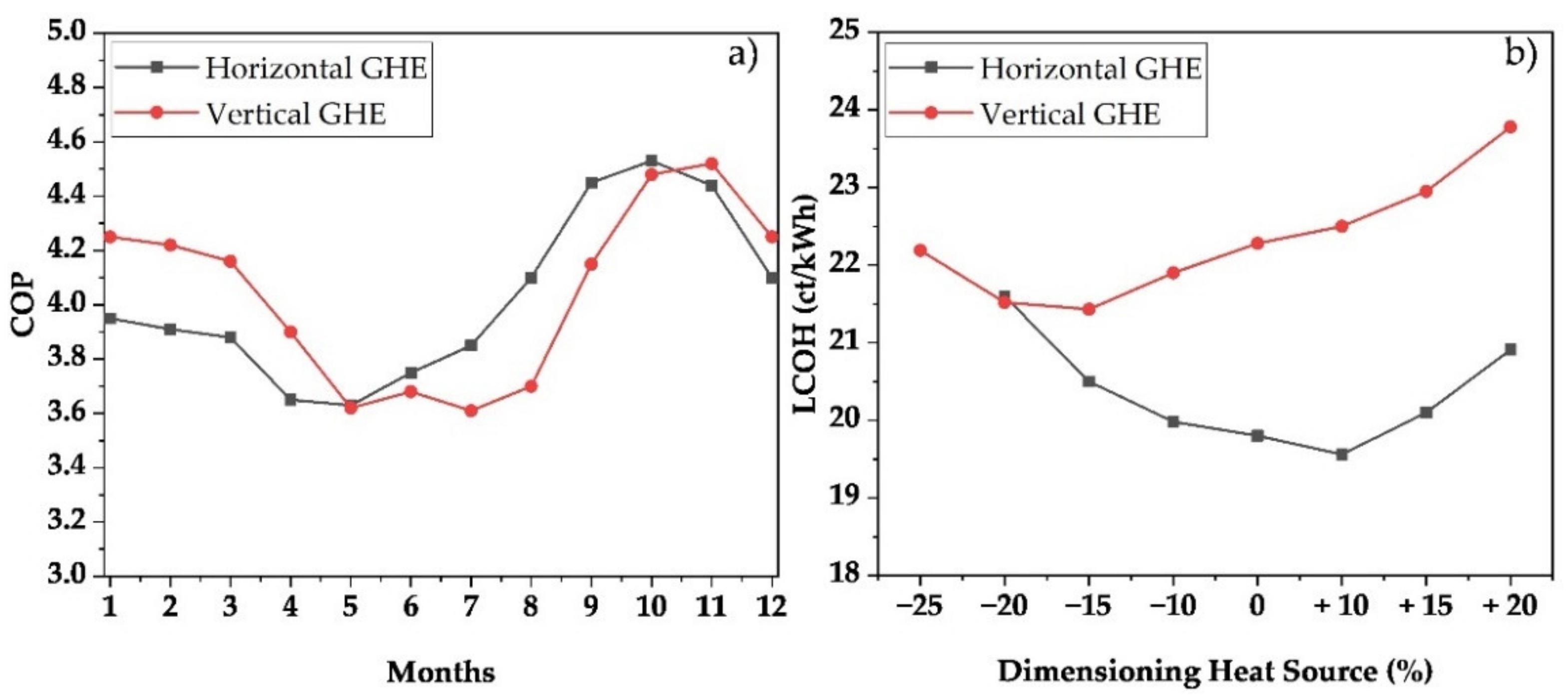
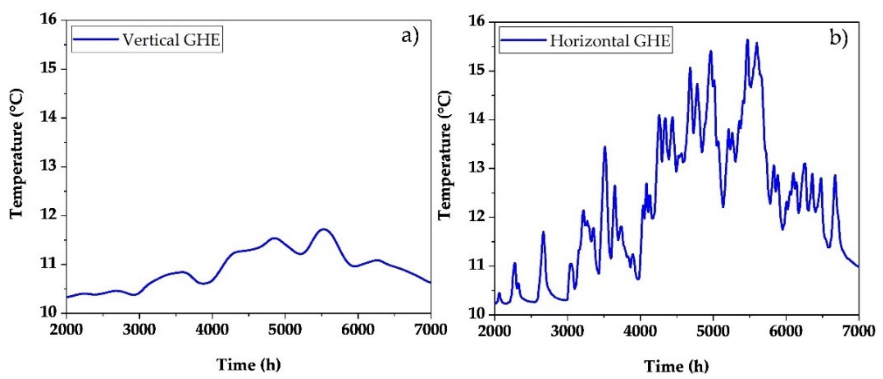
3.1. Sole Heating Case
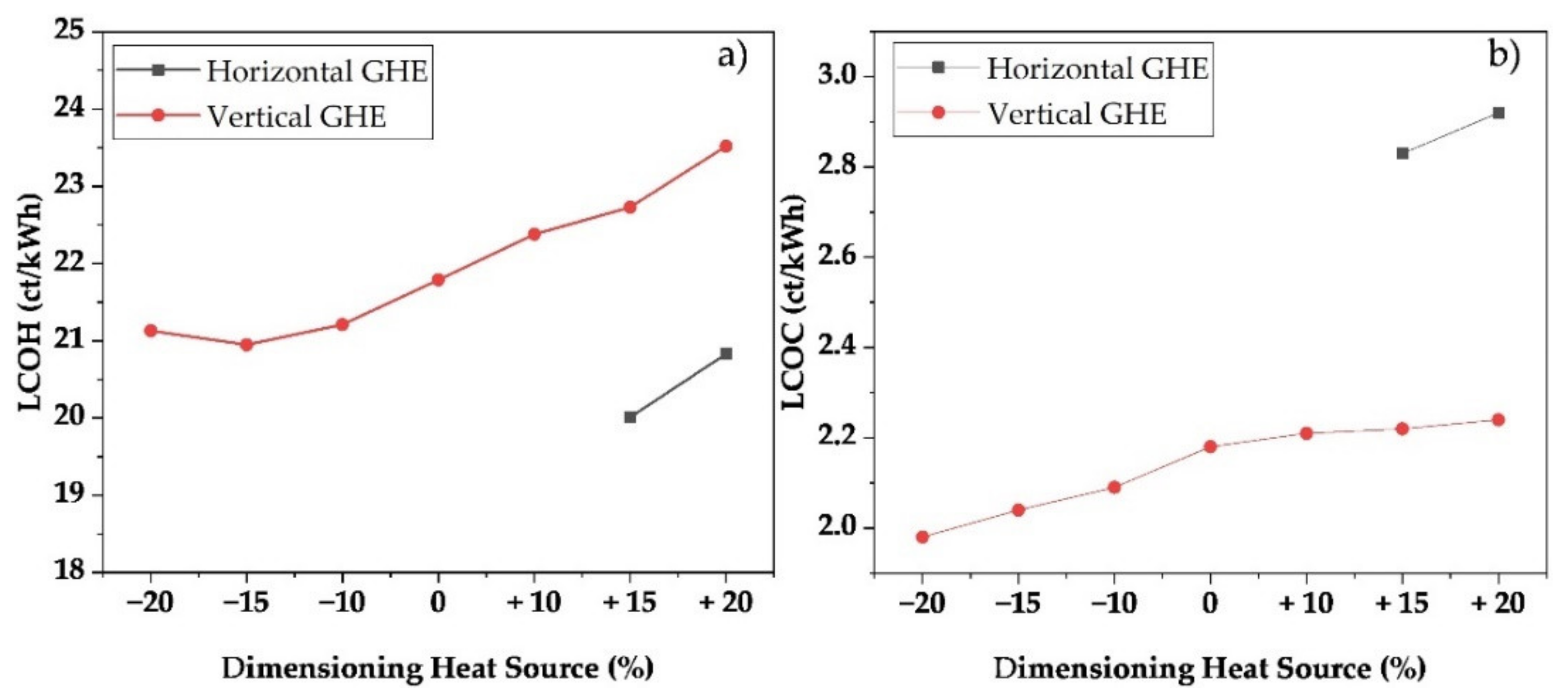
3.2. Heating and Cooling Scenario
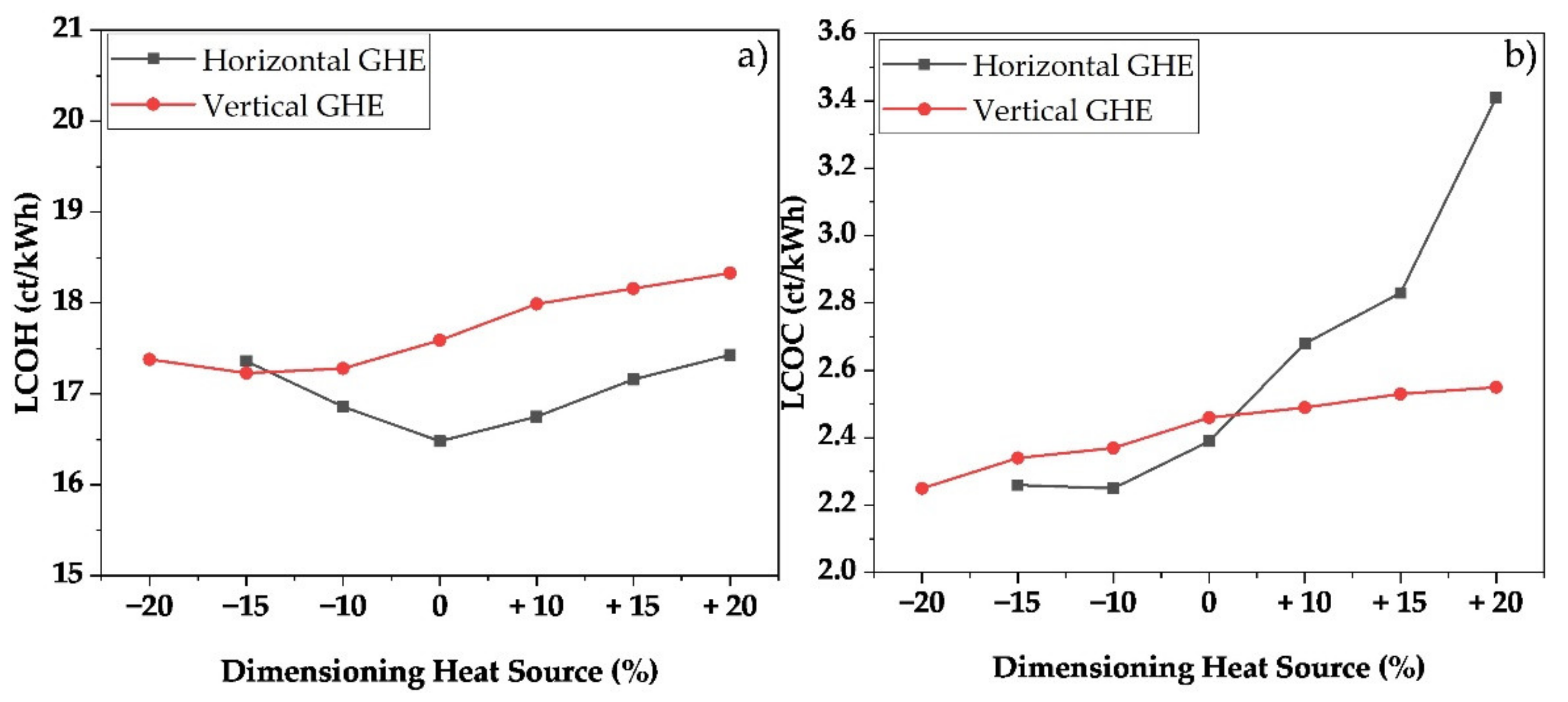
3.3. Variation of the Region
4. Conclusions
Author Contributions
Funding
Institutional Review Board Statement
Informed Consent Statement
Data Availability Statement
Conflicts of Interest
Nomenclature
| Latin Letters | |
| bi | Cash value factor |
| D | Depth below the surface (surface=0) |
| di,pipe | Inner diameter of the pipe |
| g | g-function |
| gFLS(t) | g-function evaluated for the finite line source solution |
| gCHS(t) | g-function evaluated for the cylindrical geometry |
| gILF(t) | g-function evaluated for the infinite line source solution |
| H | Borehole length |
| ks | Ground thermal conductivity |
| lpipe | Length of the pipe |
| Nb | Number of boreholes in the field |
| OMi | Sum of annual cost for operation and maintenance |
| Pi | Annualised capital cost of investment pf the specific component i |
| P0 | Investment amount of the specific component |
| Pel | Electrical power |
| pfric | Pressure losses due to friction |
| pgeo | Pressure losses due to geodetic elevation |
| Q | Heat flow |
| Qi | Annual amount of energy |
| q | Interest factor |
| R | Annual revenues |
| rpipe,inner | Inner radius of the pipe |
| rpipe,outer | Outer radius of the pipe |
| rsoil | Radius of the cylindrical soil cell |
| Tamp | Amplitude of surface temperature |
| Tb(t) | Borehole wall temperature |
| Tg | Undisturbed ground temperature |
| Tmean | Mean surface temperature (average air temperature). |
| Tsoil | Soil temperature at depth D and Time of year |
| tshift | Day of the year of the minimum surface temperature |
| tyear | Current time |
| vpipe | Velocity within the pipe |
| z | Geodetic elevation |
| Greek Letters | |
| α | Thermal diffusivity of the ground (soil) |
| ρmedium | Density of the fluid |
| λpipe | Friction factor |
| λpipe | Heat conductivity of the pipe |
| λsoil | Heat conductivity of the soil |
| Abbreviations | |
| COP | Coefficient of Performance |
| GHE | Ground Heat Exchanger |
| LCOC | Levelised Cost of Cold |
| LCOH | Levelised Cost of Heat |
| LTDH | Low-temperature district heating |
References
- European technology platform on renewable heating and cooling. In 2020–2030–2050, Common Vision for the Renewable Heating and Cooling Sector in Europe; European Union: Brussels, Belgium, 2011; Available online: https://op.europa.eu/en/publication-detail/-/publication/151b6f88-5bf1-4bad-8c56-cc496552cd54/language-en (accessed on 9 January 2022).
- Pérez-Lombard, L.; Ortiz, J.; Pout, C. A review on buildings energy consumption information. Energy Build. 2008, 40, 394–398. [Google Scholar] [CrossRef]
- Pezzutto, S.; Fazeli, R.; de Felice, M.; Sparber, W. Future development of the air-conditioning market in Europe: An outlook until 2020. WIREs Energy Environ. 2016, 5, 649–669. [Google Scholar] [CrossRef]
- Winter, W.; Haslauer, T.; Obernberger, I. Untersuchungen der Gleichzeitigkeit in kleinen und mittleren Nahwärmenetzen. Euroheat Power 2001, 9. Available online: http://www.verenum.ch/Dokumente/2001_Winter-Gleichzeitig.pdf (accessed on 9 January 2022).
- Santamouris, M. Cooling the buildings—Past, present and future. Energy Build. 2016, 128, 617–638. [Google Scholar] [CrossRef]
- Connolly, D.; Lund, H.; Mathiesen, B.V.; Werner, S.; Möller, B.; Persson, U.; Boermans, T.; Trier, D.; Østergaard, P.A.; Nielsen, S. Heat Roadmap Europe: Combining district heating with heat savings to decarbonise the EU energy system. Energy Policy 2014, 65, 475–489. [Google Scholar] [CrossRef]
- Ruesch, F.; Haller, M. Potential and limitations of using low-temperature district heating and cooling networks for direct cooling of buildings. Energy Procedia 2017, 122, 1099–1104. [Google Scholar] [CrossRef]
- Bilardo, M.; Sandrone, F.; Zanzottera, G.; Fabrizio, E. Modelling a fifth-generation bidirectional low temperature district heating and cooling (5GDHC) network for nearly Zero Energy District (nZED). Energy Rep. 2021, 13, 193. [Google Scholar] [CrossRef]
- Wang, C.; Wang, Q.; Nourozi, B.; Pieskä, H.; Ploskić, A. Evaluating the cooling potential of a geothermal-assisted ventilation system for multi-family dwellings in the Scandinavian climate. Build. Environ. 2021, 204, 108114. [Google Scholar] [CrossRef]
- Li, S.; Dong, K.; Wang, J.; Zhang, X. Long term coupled simulation for ground source heat pump and underground heat exchangers. Energy Build. 2015, 106, 13–22. [Google Scholar] [CrossRef]
- Dassault Systems. Dymola Systems Engineering. Available online: https://www.3ds.com (accessed on 9 January 2022).
- Wetter, M.; Zuo, W.; Nouidui, T.S.; Pang, X. Modelica Buildings library. J. Build. Perform. Simul. 2014, 7, 253–270. [Google Scholar] [CrossRef]
- ASHRAE. Handbook—Fundamentals: Chapter 17, Residential Cooling and Heating Load Calculations; American Society of Heating, Refrigerating and Air-conditioning Engineers: Atlanta, GA, USA, 2017. [Google Scholar]
- Van der Heijde, B.; Fuchs, M.; Tugores, C.R.; Schweiger, G.; Sartor, K.; Basciotti, D.; Müller, D.; Nytsch-Geusen, C.; Wetter, M.; Helsen, L. Dynamic equation-based thermo-hydraulic pipe model for district heating and cooling systems. Energy Convers. Manag. 2017, 151, 158–169. [Google Scholar] [CrossRef] [Green Version]
- Arce, I.D.H.; López, S.H.; Pérez, S.L.; Rämä, M.; Klobut, K.; Febres, J.A. Models for fast modelling of district heating and cooling networks. Renew. Sustain. Energy Rev. 2018, 82, 1863–1873. [Google Scholar] [CrossRef]
- MEGlobal. Ethylene Glycol Product Guide. Available online: https://www.meglobal.biz/wp-content/uploads/2019/01/Monoethylene-Glycol-MEG-Technical-Product-Brochure-PDF.pdf (accessed on 9 January 2022).
- Florides, G.; Kalogirou, S. Annual ground temperature measurements at various depths. In Proceedings of the 8th REHVA World Congress Clima 2005, Lausanne, Switzerland, 9–12 October 2005. [Google Scholar]
- Perpar, M.; Rek, Z.; Bajric, S.; Zun, I. Soil thermal conductivity prediction for district heating pre-insulated pipeline in operation. Energy 2012, 44, 197–210. [Google Scholar] [CrossRef]
- Santa, G.D.; Galgaro, A.; Sassi, R.; Cultrera, M.; Scotton, P.; Mueller, J.; Bertermann, D.; Mendrinos, D.; Pasquali, R.; Perego, R.; et al. An updated ground thermal properties database for GSHP applications. Geothermics 2020, 85, 101758. [Google Scholar] [CrossRef]
- Alpha Innotec. WZSV-Serie: Betriebsanleitung. 2019. Available online: htttps://www.alpha-innotec.de (accessed on 9 January 2022).
- Kreditanstalt für Wiederaufbau. Anlage zum Merkblatt Energieeffizient Bauen (153); KfW: Frankfurt, Germany, 2016. [Google Scholar]
- Jeong, C.-H.; Lee, J.Y.; Yeo, M.S.; Kim, K.W. Cooling Load Analysis of Residential Buildings for Dehumidification/Sub-Cooling Systems in Radiant Cooling. Sustain. Build. 2007, 1, 505–512. [Google Scholar]
- Polinder, H.; Schweiker, M.; Van der Aa, A. Occupant Behavior and Modeling; Tohoku University: Tohoku, Japan, 2013. [Google Scholar]
- Carrier. Hourly Analysis Program (HAP). Available online: https://www.carrier.com/commercial/en/us/software/hvac-system-design/hourly-analysis-program/ (accessed on 6 December 2021).
- De Santiago, J.; Rodriguez-Villalón, O.; Sicre, B. The generation of domestic hot water load profiles in Swiss residential buildings through statistical predictions. Energy Build. 2017, 141, 341–348. [Google Scholar] [CrossRef] [Green Version]
- Braas, H.; Jordan, U.; Best, I.; Orozaliev, J.; Vajen, K. District heating load profiles for domestic hot water preparation with realistic simultaneity using DHWcalc and TRNSYS. Energy 2020, 201, 117552. [Google Scholar] [CrossRef]
- Blum, P.; Campillo, G.; Kölbel, T. Techno-economic and spatial analysis of vertical ground source heat pump systems in Germany. Energy 2011, 36, 3002–3011. [Google Scholar] [CrossRef]
- Verein Deutscher Ingenieure. Thermal Use of the Underground—Fundamentals, Approvals, Environmental Aspects (4640). 2010. Available online: https://www.vdi.de/en/home/vdi-standards/details/vdi-4640-blatt-1-thermal-use-of-the-underground-fundamentals-approvals-environmental-aspects (accessed on 9 January 2022).
- Brennenstuhl, M.; Zeh, R.; Otto, R.; Pesch, R.; Stockinger, V.; Pietruschka, D. Report on a Plus-Energy District with Low-Temperature DHC Network, Novel Agrothermal Heat Source, and Applied Demand Response. Appl. Sci. 2019, 9, 5059. [Google Scholar] [CrossRef] [Green Version]
- Bauer, D.; Heidemann, W.; Müller-Steinhagen, H.; Diersch, H.-J.G. Thermal resistance and capacity models for borehole heat exchangers. Int. J. Energy Res. 2011, 35, 312–320. [Google Scholar] [CrossRef]
- Laferrière, A.; Cimmino, M.; Picard, D.; Helsen, L. Development and validation of a full-time-scale semi-analytical model for the short- and long-term simulation of vertical geothermal bore fields. Geothermics 2020, 86, 101788. [Google Scholar] [CrossRef]
- Eskilson, P. Thermal Analysis of Heat Extraction Boreholes; Lund University: Lund, Sweden, 1987. [Google Scholar]
- Cimmino, M.; Bernier, M. A semi-analytical method to generate g-functions for geothermal bore fields. Int. J. Heat Mass Transf. 2014, 70, 641–650. [Google Scholar] [CrossRef]
- Cimmino, M. Fast calculation of the g -functions of geothermal borehole fields using similarities in the evaluation of the finite line source solution. J. Build. Perform. Simul. 2018, 11, 655–668. [Google Scholar] [CrossRef] [Green Version]
- Li, M.; Li, P.; Chan, V.; Lai, A.C.K. Full-scale temperature response function (G-function) for heat transfer by borehole ground heat exchangers (GHEs) from sub-hour to decades. Appl. Energy 2014, 136, 197–205. [Google Scholar] [CrossRef]
- Sangi, R.; Müller, D. Dynamic modelling and simulation of a slinky-coil horizontal ground heat exchanger using Modelica. J. Build. Eng. 2018, 16, 159–168. [Google Scholar] [CrossRef]
- Verein Deutscher Ingenieure. Economic Efficiency of Building Installations. 2012. Available online: https://www.vdi.de (accessed on 9 January 2022).
- Brennenstuhl, M. Sektorkopplung mit kalter Nahwärme aus Geothermie—intelligenter Energieaustausch am Beispiel einer Plusenergiesiedlung in Wüstenrot, HFT Stuttgart. 2019. Available online: https://docplayer.org/112222856-Waerme-aus-dem-acker-agrothermie-und-kaltwaermenetz.html (accessed on 9 January 2022).
- Strom-Report. Strompreise. 2021. Available online: https://strom-report.de/strompreise/ (accessed on 6 December 2021).
- Roy, C. Review of Discretization Error Estimators in Scientific Computing. In Proceedings of the 48th AIAA Aerospace Sciences Meeting Including the New Horizons Forum and Aerospace Exposition, Orlando, FL, USA, 4–7 January 2010; American Institute of Aeronautics and Astronautics: Reston, VA, USA, 2012; p. 1, ISBN 978-1-60086-959-4. [Google Scholar]


| Parameter | Value | Unit |
|---|---|---|
| Material | Polyethylene 100 | |
| Inner diameter | 25–150 | mm |
| Wall thickness | 3–6 | mm |
| Thermal conductivity | 0.42 | W/(m·K) |
| Pipe roughness | 0.0014 | mm |
| Parameter | Value | Unit |
|---|---|---|
| Share of ethylene glycol | 20 | vol% |
| Freezing point | −8 | °C |
| Density | 1028 | kg/m³ |
| Specific heat capacity | 3.97 | kJ/(kg·K) |
| Viscosity | 2 × 10⁻³ | Pa·s |
| Parameter | Value | Unit |
|---|---|---|
| Ground thermal capacity | 2.6 | MJ/(m³·K) |
| Ground thermal conductivity | 1.5–3.5 | W/(m·K) |
| Ground thermal diffusivity | 9.77 × 10⁻⁷ | m/s² |
| Depth where the temperature gradient starts | 10 | m |
| Vertical temperature gradient | 0.03 | K/m |
| Building Component | Thermal Transmittance [W/(m²·K)] |
|---|---|
| Roof surfaces, top floor ceiling | 0.14 |
| Transparent building components | 0.9 |
| Opaque components | 0.25 |
| Basement | 0.2 |
| Exterior walls | 0.2 |
| Cellar and exterior doors | 1.2 |
| Parameter | Value | Unit |
|---|---|---|
| Diameter geothermal pipes | 32 | mm |
| Wall thickness pipe | 3 | mm |
| Heat conductivity pipe | 0.42 | W/(m·K) |
| Type of vertical GHE | Double U-pipe | - |
| Distance between U-pipes | 5 | m |
| Maximum drilling depth | 100 | m |
| Borehole radius | 75 | mm |
| Density grout | 1600 | kg/m³ |
| Heat conductivity grout | 0.81 | W/(m·K) |
| Heat capacity grout | 800 | J/(kg·K) |
| Depth of the horizontal GHE | 1.5 | m |
| Distance between horizontal pipes | 0.7 | m |
| Parameter | Value | Unit | Reference |
|---|---|---|---|
| Installation of LTDH network | 230 | €/m | [28,38] |
| Maintenance of LTDH network | 1 | % of total invest/a | [37] |
| Installation vertical GHE | 1050 | €/kW | [27] |
| Installation horizontal GHE | 450 | €/kW | [38] |
| Consumer heat pump | 1000 | €/kW | [27] |
| Substation and installation | 4000 | € | - |
| Interest factor | 1.05 | - | [37] |
| Price change factor | 1.03 | - | [37] |
| Observation period | 40 | a | [37] |
| Electricity tariff for heat pumps | 22.5 | ct/kWhel | [39] |
| Parameter | Value | Unit |
|---|---|---|
| Number of consumers | 41 | – |
| Total length of the grid | 650 | m |
| Geothermal extraction power | 200 | kW |
| Room heating demand per consumer | 5224 | kWh/a |
| Domestic hot water demand per consumer | 3276 | kWh/a |
| Calculated cooling demand per consumer | 3938 | kWh/a |
| Vertical GHE | Horizontal GHE | |
|---|---|---|
| Design case | 0% | 0% |
| Total invest heat source (€) | 210,000 | 90,000 |
| Mean value COP | 4.15 | 3.98 |
| Electricity demand (kWhel) | 2048 kWh | 2135 |
| LCOH (ct/kWh) | 22.28 | 19.80 |
| Optimal case | −15% | +10% |
| Invest cost heat source (€) | 178,500 | 99,000 |
| Mean value COP | 3.79 | 4.17 |
| Electricity demand (kWhel) | 2242 | 2036 |
| LCOH (ct/kWhth) | 21.43 | 19.56 |
| Savings (%) | 3.8 | 1.5 |
| Stuttgart | Oslo | Bordeaux | |
|---|---|---|---|
| Annual mean ambient temperature (°C) | 10.1 | 7.0 | 13.9 |
| Annual amount of heating energy (kWh) | 5224 | 8839 | 1729 |
| Annual amount of cooling energy (kWh) | 3938 | 3057 | 6294 |
| Annual domestic hot water load (kWh) | 3276 | 3276 | 3276 |
| Design installation cost vertical GHE (€) | 210,000 | 296,100 | 123,900 |
| Design installation cost horizontal GHE (€) | 90,000 | 126,900 | 53,100 |
| Stuttgart | Oslo | Bordeaux | Madrid | |
|---|---|---|---|---|
| Annual heat demand per consumer [kWh] | 8500 | 12,115 | 5005 | 4321 |
| Annual cooling demand per consumer [kWh] | 3938 | 3057 | 6294 | 9677 |
| Heating-to-cooling demand ratio | 2.2 | 4.0 | 0.8 | 0.4 |
| Most economic GHE system | Horizontal | Horizontal | Vertical | Vertical |
| Savings from next most economic GHE [%] | 2.65 | 4.16 | 3.00 | - |
Publisher’s Note: MDPI stays neutral with regard to jurisdictional claims in published maps and institutional affiliations. |
© 2022 by the authors. Licensee MDPI, Basel, Switzerland. This article is an open access article distributed under the terms and conditions of the Creative Commons Attribution (CC BY) license (https://creativecommons.org/licenses/by/4.0/).
Share and Cite
Kutzner, S.; Heberle, F.; Brüggemann, D. Thermo-Economic Analysis of Near-Surface Geothermal Energy Considering Heat and Cold Supply within a Low-Temperature District Heating Network. Processes 2022, 10, 421. https://0-doi-org.brum.beds.ac.uk/10.3390/pr10020421
Kutzner S, Heberle F, Brüggemann D. Thermo-Economic Analysis of Near-Surface Geothermal Energy Considering Heat and Cold Supply within a Low-Temperature District Heating Network. Processes. 2022; 10(2):421. https://0-doi-org.brum.beds.ac.uk/10.3390/pr10020421
Chicago/Turabian StyleKutzner, Sebastian, Florian Heberle, and Dieter Brüggemann. 2022. "Thermo-Economic Analysis of Near-Surface Geothermal Energy Considering Heat and Cold Supply within a Low-Temperature District Heating Network" Processes 10, no. 2: 421. https://0-doi-org.brum.beds.ac.uk/10.3390/pr10020421