Research on Mixing Behavior in a Combined Top–Bottom–Side Blown Iron Bath Gasifier

Abstract

The iron bath gasifier studied in this paper is a new type of reactor for handling organic solid waste, in which the complex transport phenomena comprising high temperature, the multiphase flow, mixing, and chemical reaction takes place. It is of great significance to study the melt’s flow and mass transfer behavior in this reactor. The influence of different process parameters on the mixing behavior of the molten pool was studied by the water modeling experiment and numerical simulation method. The experimental results show that the height of the water phase has a highly significant effect on the mixing time of the molten pool, followed by the horizontal angle of the side gun and the bottom blowing flow rate. As the height of the water increases, the mixing time decreases. When the horizontal angle of side lances increases, the mixing time decreases. With the increase in the flow rate of the bottom lance, the mixing time decreases. The results obtained by numerical simulation were compared with the experimental results to determine the reliability of the mathematical model for future optimization of the process parameters by numerical simulation. These studies are helpful for optimizing the design of the reactor and improving the process parameters.

1. Introduction

With the increasingly severe global climate crisis, green, low-carbon, and sustainable development have become the consensus of every country globally. In 2020, China proposed to achieve carbon peaking by 2030 and carbon neutrality by 2060 [1]. In this context, the steel industry vigorously promotes low-carbon metallurgy and eliminates backward and excess capacity. The traditional waste treatment process brings much pollution. Converting the abandoned converter into a solid waste reactor [2] solves the problem of organic waste treatment and helps to save energy and reduce carbon. Niu et al. [2] disclosed a double-melt bath organic solid waste blowing gasification device. Organic matter particles to be gasified are immersed and sprayed into a melt bath, while gasifying agents such as oxygen and oxygen-enriched air are bubbled into the melt; the organic matter is gasified into a synthesis gas that is rich in CO and hydrogen. The present process can gasify the vast majority of organic waste into clean combustible gas, which can be used as fuel gas or chemical product synthesis gas. It reduces carbon emissions and is beneficial to carbon neutralization. In the converter reactor, the thermochemical decomposition of organic solid waste particles injected into the bath takes place under the condition of iron liquid as the catalyst and high temperature. By blowing nitrogen from the bottom lance and oxygen from the top lance and side lance, the stirring effect of the molten pool is enhanced, the mass transfer and reaction rate are improved, and the temperature in the molten pool is promoted to be uniform. Therefore, it is of great significance to study the flow and mass transfer behavior in the molten pool under different injection processes.

Due to the high temperature in the converter, it is difficult to investigate the flow patterns in the furnace. Therefore, scholars mostly use the methods of physical simulation and numerical simulation to study the behavior of multiphase flow in the molten pool [3,4,5,6,7,8,9,10]. Wu et al. [11] carried out a numerical simulation of gas–liquid two-phase flow in the converter, studied the influence of the bottom blowing flow rate and the bottom blowing port position on the flow field of the molten steel, and optimized the bottom blowing system. Li et al. [12] conducted a numerical simulation of gas–liquid two-phase flow in a converter with top–bottom blowing and studied the effect of the distribution of the bottom blowing and the height of the top lance on the gas–liquid flow. Chu et al. [13] studied the effects of the bottom blowing gas flow rate distribution patterns and the bottom blowing gas flow distribution gradients on the flow field patterns, mixing time, and liquid steel–slag interface velocity in a top–bottom combined blowing converter by numerical simulation. Zhou et al. [14,15,16] established a top blowing model, a top–bottom blowing model, and a top–bottom side blowing model, respectively, and studied the effects of different blowing positions and flow rates on the flow patterns and mixing times. Shota et al. [17] studied the effects of top blowing and bottom blowing conditions on the splashing behavior of converters through water model experiments and numerical simulations. The interference between the top-blown jet and the bottom-blown plume was found to increase the airflow velocity at the cavity edge, resulting in increased spattering. Zhong et al. [18] studied the effect of side blowing on the flow of molten pools by using water modeling and found that side blowing can enhance the stirring effect and significantly reduce the mixing time of the molten pool. Fabritius [19] established a physical model of a smelting chromium converter, adding side blowing and top blowing. The experimental results show that side blowing increases the penetration depth of the molten pool and shortens the mixing time by about one-third. Christian et al. [20] studied the effect of the side lance flow rate and the filling level on the mixing time for AOD furnaces using a water model. Patrik et al. [21] studied the mixing time of the side-blown converter by means of a water model experiment and found that the mixing time was affected by the gas flow rate and the diameter of the vessel, but not by the height of the molten pool. Serg et al. [22] studied the effect of the converter inclination on the mixing time and the jet penetration length with a side-blown water model and found that the penetration length is shown to be independent of the inclination angle, and the mixing time was affected by the intensified wave motion at the interface caused by the inclination of the vessel. Xie et al. [23,24] conducted a physical simulation of the three-phase flow behavior of gas–liquid–slag in a C-H₂ iron bath furnace and studied the effects of factors such as the flow rate and angle of the double-row side lances, and the position where the tracer was added on the average residence time and obtained the expression between the mixing time and the dimensionless group through multiple linear regression. The experimental verification shows that the calculated value positively correlates with the experimental value. Zhu et al. [25] studied the effects of different parameters on the mass transfer and mixing behavior of the side-blown vortex smelting reduction reactor by physical simulation and obtained the relationship between the dimensionless number and the mixing time by using a dimensional analysis. Zhang et al. [26] conducted a dimensional analysis on the mixing time of the top–bottom–side-blown furnace to explore the internal relationship between different factors.

Previous scholars’ studies [12,13,14,15,16,17,18,19,20,21,22] on iron bath furnaces mainly focus on top–bottom blowing or side blowing, and there are few studies on top–bottom–side-combined blowing. The top–bottom–side-blown iron bath gasifier studied in this paper is a new type of solid waste reactor which is transformed from a converter. Air and raw materials are blown at the top, oxygen-enriched air is blown at the bottom, and oxygen is blown at the side lances to stir the melting pool. The molten pool is fully stirred by the combined blowing technology so that the heat of the top layer is transferred downward, the flow of the molten steel and the slag layer is strengthened, the mass transfer rate is increased, the dead zone is reduced, and the mixing time of the molten pool is reduced. In the current study, the stirring effect on the molten pool is mainly analyzed based on process factors such as the flow rate of the bottom blowing lance and side blowing lance, the immersion depth and angle of the side lance, the position of the top lance, the height of the water and oil phases, and the feeding height of the tracer. These conclusions obtained are also widely applicable to optimize the reactor’s design and improve the process parameters.

2. Models and Methods

2.1. Physical Model and Methods

In order to make the model used in the water simulation experiment truly reflect the actual process, the model and the prototype should conform to the principle of similarity, that is, geometric similarity and dynamic similarity [27]. Due to the limitation of physical experimental conditions, it is usually necessary to scale the model in equal proportions. In this paper, the ratio of the model to prototype is 1:8. For kinetic similarity, the dimensionless Reynolds number and the Froude number are usually used. In the research process, the flow in the reactor is mainly driven by gas stirring rather than turbulent viscous force. That is, buoyancy and inertial force will mainly control the movement of gas. Therefore, it is usually based on the Froude number, and considering the gas phase expansion factor, the modified Froude number [28] is generally used for research, such as Formula (1).

$$Fr’=\frac{u^2}{gd}\times \frac{{\rho }_g}{{\rho }_l-{\rho }_g}$$

(1)

where $u$ is the speed, m/s; $g$ is the acceleration of gravity, m/s²; $d$ is the characteristic size; ${\rho }_l$is the liquid density; ${\rho }_g$ is the gas density.

In the water model experiment, water is used to simulate molten steel, high vacuum oil is used to simulate slag, and air is used to simulate oxygen and oxygen-enriched air. The physical property parameters of the various materials used in the experiment are shown in

Table 1. Physical property parameters of materials.

Material	Density (kg·m−3)	Viscosity (kg·m−1·s−1)
Steel	7000	0.0063
Slag	3000	0.4
Air	1.205	1.79 × 10−5
Water	1000	0.001
Oil	860	0.0753

.

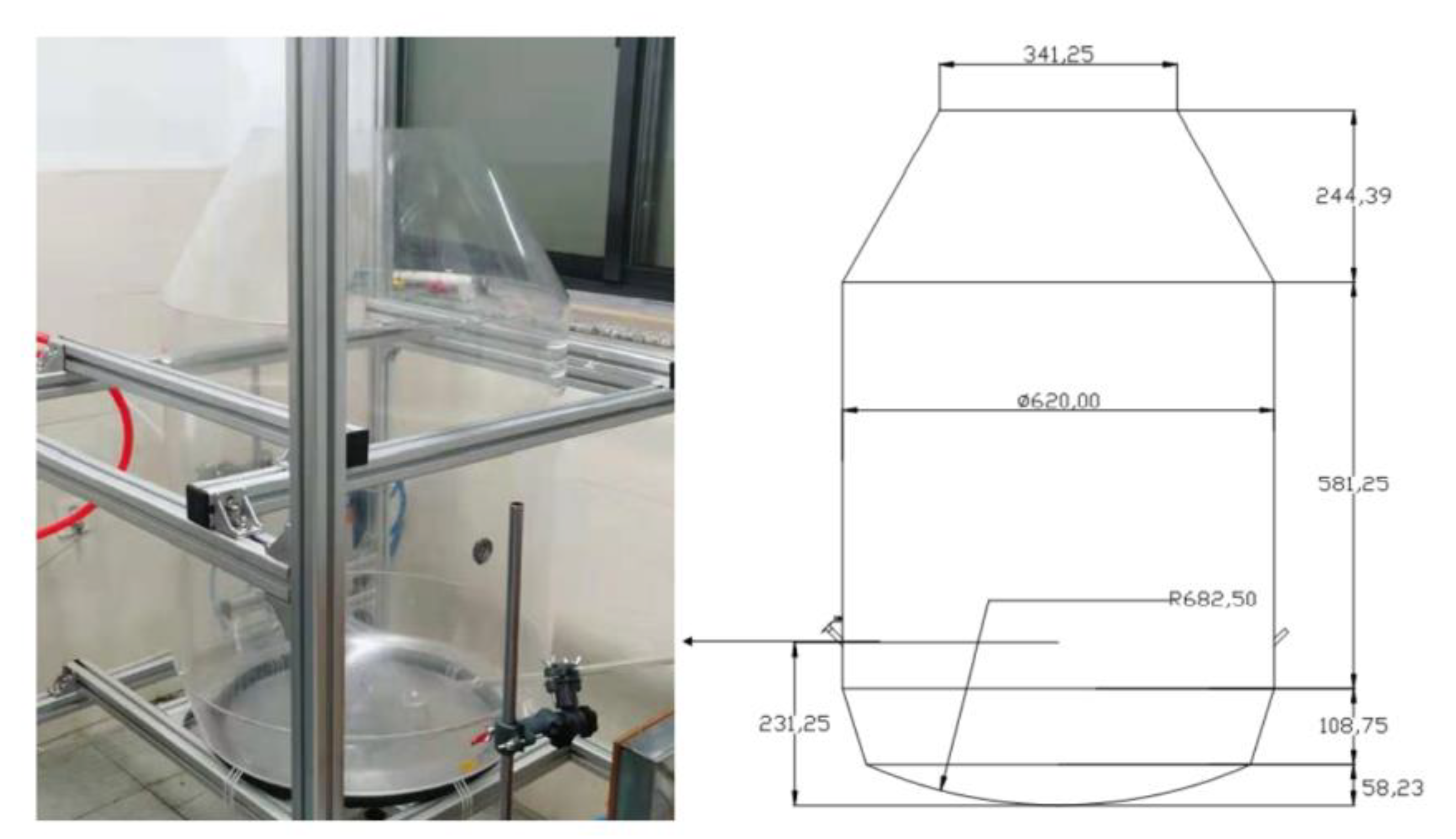
The experimental equipment includes a screw air compressor with a gas storage tank, a split flow and steady flow device, a simulated reaction furnace, and a data monitoring and acquisition system, as shown in Figure 1. The air compressor equipment is a screw air compressor with a power of 7.5 kw, and the model is 7.5MV-8-G. The gas steady flow device is self-made. Using the DDS-IIA conductivity meter and the matching DSJ-1 electrode probe, the electrical signal collected by the conductivity meter is converted into a digital signal by the DJ800 data monitoring system, and then recorded and displayed on the computer by the Self-programmed data acquisition software system. A 120t converter model with a similarity ratio of 1:8 is made of plexiglass. The shape and size of the model are shown in Figure 2 and

Table 2. Prototype and model size parameters.

Geometric Parameters	Prototype	Model
Height of reactor (mm)	7941	993
Diameter of furnace (mm)	4960	620
Diameter of oxygen lance (mm)	145	18
Diameter of side lance (mm)	60	8

, respectively.

The three monitoring points were selected to measure the mixing time of the tracer in the bath. They are located at the horizontal surface of 45 mm height, with a 120° angle between each point, as shown in Figure 3.

In this paper, orthogonal experiments are used to explore the relationship between the nine process factors and the mixing time. The specific parameters of each factor are shown in

Table 3. Experimental parameters of water model.

Factor		Parameter
Top lance	Position (mm)	90, 180, 270
	Flow rate (m3·h−1)	5
Bottom lance	Flow rate (L·min−1)	3, 6, 9
Side lance	Insertion depth (mm)	0, 25, 50
	Vertical angle (°)	15, 30, 45
	Horizontal angle (°)	15, 30, 46
	Flow rate (m3·h−1)	8, 13, 18
Water	Height (mm)	60, 75, 90
Tracer	Height (mm)	90, 135, 180
Oil	Height (mm)	120, 160, 200

. In this water modeling experiment, three positions of the top lance are considered to study the influence of the position on the mixing of the molten pool. Only three different flow rates of bottom blowing are studied since the bottom blowing position is fixed. In order to facilitate the transformation of the converter, double-sided lances with fixed positions are used, and the influence of the flow rate, angle, and immersion depth of the side lances on the mixing time of the molten pool are considered. The selection of the horizontal and vertical angles is shown in Figure 4, the angle between the side lance and the radial line is the horizontal angle, and the angle between the side lance and the horizontal line is the vertical angle. Since the bottom of the reactor is the inclined wall, the reaction interface area of the water–oil (the molten steel and the slag layer) increases with the increase of the height of the water. When the flow conditions of different heights of the slag layer are different, the position where different tracers are added will also affect the measurement of the mixing time.

2.2. Numerical Model and Methods

2.2.1. VOF Model

The VOF model is a surface-tracking technique applied to a fixed Eulerian mesh. It is designed for two or more immiscible fluids where the position of the interface between the fluids is of interest. In the VOF model, a single set of momentum equations is shared by the fluids, and the volume fraction of each of the fluids in each computational cell is tracked throughout the domain. For the q phase, the mass conservation equation is as follows [29]:

$$\frac{\partial }{\partial t}\left({\alpha }_q{\rho }_q\right)+\nabla \cdot \left({\alpha }_q{\rho }_q{\overrightarrow{v}}_q\right)=0$$

(2)

where ${\alpha }_q$ is the volume fraction of the $q$ phase and ${\rho }_q$ is the density of the $q$ phase.

A single momentum equation is solved throughout the domain, and the resulting velocity field is shared among the phases. The momentum equation [29], shown below, is dependent on the volume fractions of all phases through the properties $\rho$ and $\mu$.

$$\frac{\partial }{\partial t}\left(\rho \overrightarrow{v}\right)+\nabla \cdot \left(\rho \overrightarrow{v}\overrightarrow{v}\right)=-\nabla P+\nabla \cdot \left[\mu \left(\nabla \overrightarrow{v}+\nabla {\overrightarrow{v}}^T\right)\right]+\rho g+\overrightarrow{F}$$

(3)

where $\rho$ and $\mu$ are the density and molecular viscosity coefficients, respectively, $P$ is the pressure, and $\overrightarrow{F}$ is the source term.

2.2.2. Turbulence Model

The standard k-ε model is used to describe the turbulent kinetic energy (k) and the turbulent kinetic energy dissipation rate (ε), and the calculation formula [29] is as follows:

$$\frac{\partial }{\partial t}\left(\rho k\right)+\frac{\partial }{\partial x_i}\left(\rho \kappa u_i\right)=\frac{\partial }{\partial x_j}\left[\left(\mu +\frac{{\mu }_t}{{\sigma }_{\kappa }}\right)\frac{\partial \kappa }{\partial x_j}\right]+G_k-\rho \epsilon$$

(4)

$$\frac{\partial }{\partial t}\left(\rho \epsilon \right)+\frac{\partial }{\partial x_i}\left(\rho \epsilon u_i\right)=\frac{\partial }{\partial x_j}\left[\left(\mu +\frac{{\mu }_t}{{\sigma }_{\epsilon }}\right)\frac{\partial \epsilon }{\partial x_j}\right]+\frac{\epsilon }{k}\left(C_{1\epsilon }{G}_k-C_{2\epsilon }\rho \epsilon \right)$$

(5)

where $G_k$ represents the turbulent kinetic energy due to the mean velocity gradient, ${\sigma }_{\kappa }$and ${\sigma }_{\epsilon }$are the turbulent Prandtl numbers for $k$ and $\epsilon$, and ρ and μ are the density and molecular viscosity coefficients. The turbulent (or eddy) viscosity, ${\mu }_t$, is computed by combining $k$ and $\epsilon$ as follows [29]:

$${\mu }_t=\rho C_{\mu }\frac{k^2}{\epsilon }$$

(6)

$C_{1\epsilon }$, $C_2$, $C_{\mu }$, ${\sigma }_{\kappa }$, and ${\sigma }_{\epsilon }$ are empirical constants, and the coefficients used in this paper are taken from the recommended values of Launder and Spalding [30]. $C_{1\epsilon }=1.44,C_{2\epsilon }=1.92,C_{\mu }=0.09,{\sigma }_k=1.0,{\sigma }_{\epsilon }=1.3$.

2.2.3. Species Transport Model

In order to determine the mixing time in the molten pool, the diffusion equation of the tracer, that is, the component transport equation, is solved in the reactor. The conservation equation is expressed as follows [29]:

$$\frac{\partial }{\partial t}\left(\rho Y_i\right)+\nabla ·\left(\rho \overrightarrow{v}{Y}_i\right)=-\nabla ·\overrightarrow{J_i}$$

(7)

where $Y_i$ is the local mass fraction of each species and $\overrightarrow{J_i}$ is the diffusion flux of species, which arises due to gradients of concentration. The diffusion flux of species $\overrightarrow{J_i}$ is calculated by the following formula [29]:

$${\overrightarrow{J}}_i=-\left(\rho D_{i,m}+\frac{{\mu }_t}{S{c}_t}\right)\nabla Y_i$$

(8)

where $S{c}_t$is the turbulent Schmidt number ($\frac{{\mu }_t}{\rho D_t}$ where ${\mu }_t$is the turbulent viscosity and $D_t$is the turbulent diffusivity). The default value of is 0.7. $D_{i,m}$ is the mass diffusion coefficient for species in the mixture.

2.3. Boundary Conditions and Solution Methods

The numerical simulation adopts the geometric ratio of 1:1 to simulate the water model. The dimensions are shown in Table 2, and the material and physical parameters are shown in Table 1. The boundary conditions to be solved are as follows: (1) The inlets of the top lance, bottom lance, and side lance are all velocity inlets. The velocity is obtained from the flow rate and cross-sectional area of each lance. (2) The outlet is set as a pressure outlet. The pressure is one atmosphere, that is, the relative static pressure is set to 0. (3) The wall is a nonslip wall, and the velocity is set to 0. A standard wall function is adopted near the walls.

The following assumptions are made for the simulated fluid: (1) the flow process is an isothermal process; (2) water, oil, and air are all Newtonian viscous fluids; (3) the deformation, rupture, and aggregation of the bubbles are ignored.

The calculations were performed using the VOF model, using the transient solver. In order to ensure the robustness of the calculation, an initial time step of 10^-5 s is adopted. The solution method adopts the PISO algorithm to solve the coupling problem of pressure and velocity. The pressure term is discretized in PRESTO format, the phase interface discretization scheme is in compressive format, and the rest are in the second-order upwind format. When the residual is less than 10^-3, the solution is considered to have converged at that time step. The CFD software used for numerical simulation is ANSYS Fluent.

3. Results and Discussions

The orthogonal tests of the top–bottom–side-combined blown were carried out based on a nine-factor, three-level design. The mixing time was measured by the conductivity of three electrodes in the water modeling and was calculated by the numerical simulation method. The mixing time was defined as the period required for an instantaneous tracer concentration to settle within 5% deviation around the final tracer concentration in the iron bath [31].

3.1. Orthogonal Test Analysis

The analysis of the range and variance in the orthogonal test were carried out to analyze the significant order and degree of the influence of the nine factors on the mixing time.

Table 4. Range analysis.

Factor	A *	B *	C *	D *	E *	F *	G *	H *	I *
K1	2738.4	2201.2	2276.1	2470.6	2344.2	1946.9	1858.1	1558.0	1855.9
K2	1778.1	2327.3	2086.5	2027.2	1579.6	1911.8	2030.6	2281.3	2031.4
K3	1352.4	1340.5	1506.3	1371.1	1945.2	2010.3	1980.2	2029.7	1981.7
${\stackrel{-}{\mathrm{K}}}_1$	304.3	244.6	252.9	274.5	260.5	216.3	206.5	173.1	206.2
${\stackrel{-}{\mathrm{K}}}_2$	197.6	258.6	231.8	225.2	175.5	212.4	225.6	253.5	225.7
${\stackrel{-}{\mathrm{K}}}_3$	150.3	148.9	167.4	152.3	216.1	223.4	220.0	225.5	220.2
R	154.0	109.6	85.5	122.2	85.0	10.9	19.2	80.4	19.5
sequence	A > D > B > C > E > H > I > G > F

*: A is the height of the water (mm), B is the flow rate of bottom lance (L/min), C is the flow rate of side lance (m³/h), D is the horizontal angle of side lance (°), E is the vertical angle of side lance (°), F is the insertion depth of side lance (mm), G is the height of the oil (mm), H is the height of the tracer (mm), and I is the position of the top lance (mm), the same below.

shows the results of the range analysis of the mixing time of the molten pool. The height of the water phase has the greatest influence on the mixing time, with a value of 154.0 s, followed by the horizontal angle of the side lance, with a value of 122.2 s. The least effect on the mixing time is the insertion depth of the side lance, with a value of only 10.9 s. The sequence of the influence of each factor on the mixing time is as follows: the height of water > the horizontal angle of side lance > the flow rate of bottom lance > the flow rate of side lance > the vertical angle of side lance > the height of tracer > the position of top lance > the height of oil > the insertion depth of side lance.

In the range analysis, the variation of mixing time was attributed to the level variation of each influencing factor, and the experimental error was not considered. In order to consider the influence of errors and accurately estimate the importance of the influence of various factors on the mixing time, the analysis of variance was carried out on the mixing time. The results of the analysis of variance are shown in

Table 5. Analysis of variance.

Factor	Degrees of Freedom	Adj SS	Adj MS	F	P
A	2	112,017	56,008.6	9.2	0.008
B	2	64,087	32,043.6	5.27	0.035
C	2	35,749	17,874.7	2.94	0.111
D	2	67,999	33,999.7	5.59	0.03
E	2	32,499	16,249.5	2.67	0.129
F	2	554	276.9	0.05	0.956
G	2	1747	873.6	0.14	0.868
H	2	29,964	14,982.1	2.46	0.147
I	2	1819	909.3	0.15	0.864
Error	8	48,689	6086.1
Total	26	395,125

. In the results of the ANOVA, Adj SS represents the adjusted sum of squares, and Adj MS represents the adjusted mean square. The degree of influence of each factor on the mixing time can be obtained through the p-value. When p < 0.01, it means that this factor has a very significant influence on the mixing time. When 0.01 < p < 0.05, this factor has a significant effect on the mixing time. When p > 0.05, it means that the influence of this factor on the mixing time is not significant. It can be seen from Table 5 that the most significant factor affecting the mixing time is the height of the water, and the factors that significantly affect the mixing time are the horizontal angle of the side lance and the flow rate of the bottom lance, and the other factors have no significant effect on the mixing time. Compared with the results obtained by the range analysis, it is found that the order of the influence degree of each factor on the mixing time calculated by the two methods is consistent.

The orthogonal experiment analysis shows that the optimal operating parameter scheme is the combination of A2B3C3D3E2F2G1H1I1.

3.2. Influencing Factors of Mixing Time in Top–Bottom–Side-Combined Blowing

The most significant factor affecting the mixing time is the height of the water. Figure 5 is the comparison of the mixing time at different heights of water. When the height of the water is 90 mm, the mixing time of the molten pool is the shortest. The previous discussions [18,21] on this factor are mostly based on the gas–liquid two-phase flow, and the conclusion is that the influence of the height of the water phase on the mixing time is negligible. The current model is aimed at the gas–liquid slag multiphase flow. Due to the thick slag layer process, the height of the water phase is relatively low, and the influence of the height of the water phase on the mixing time is more due to the geometric model itself. The bottom of the current model resembles an upside-down frustum. When the height of the water increases, the water–oil interface area increases, and the mixing time in the molten pool is shortened.

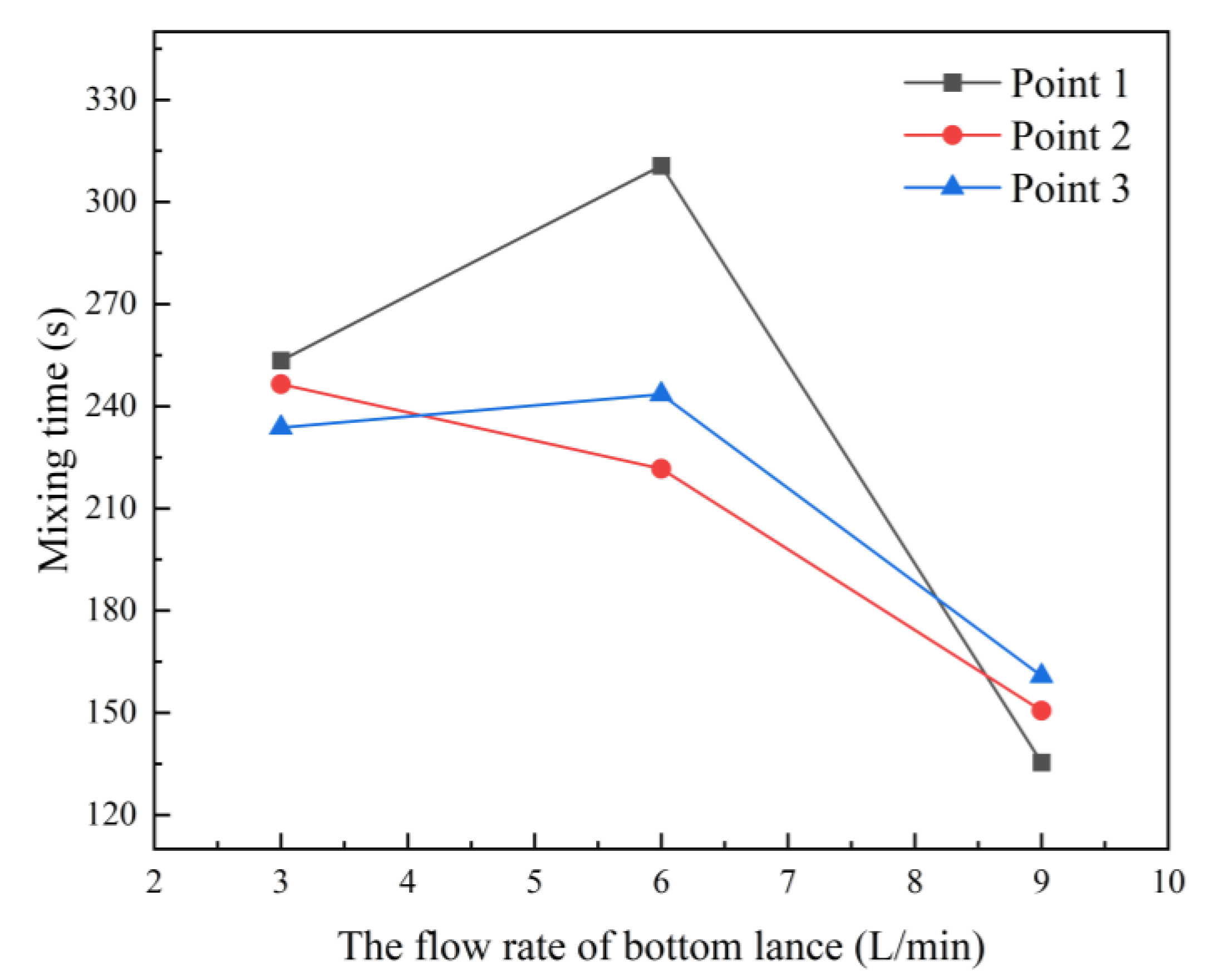
The factors that significantly affect the mixing time are the horizontal angle of the side lance and the flow rate of the bottom lance. Side-blowing is the main driving force to strengthen the movement of the slag layer. Figure 6 is the comparison of the mixing time at different horizontal angles of the side lances. The side lance is offset by a certain angle in the horizontal direction, which will drive the oil layer to generate a rotating flow field and promote the transfer of material and energy in the molten pool. In the range from 15° to 45°, as the horizontal angle of the side lance increases, the mixing time is significantly reduced, which is consistent with the trend obtained by Zhu et al. [25] at a high flow rate of the side lance. Figure 7 shows the mixing time under different flow rates of bottom blowing. At a lower flow rate of the bottom blowing, the flow in the molten pool is mainly driven by the gas blown from the side lances, and the mixing time does not change significantly. When the flow rate of the bottom blowing increases to 9L/min, the mixing time decreases significantly.

3.3. Model Validation

The accuracy of the mathematical calculation model is verified by comparing the results obtained from the numerical simulation with the results obtained from the water model experiment. Figure 8a is a plot of the measured conductivity over time in the water model, with a mixing time of 406 s. Figure 8b shows the change curve of the tracer concentration at the monitoring point in the numerical simulation, and the mixing time is 420 s. The error of the mixing time obtained by the numerical simulation and the water model experiment is within 4%, so it is determined that the results of the numerical simulation and the water model experiment have good agreement.

At the same time, the topography of the molten pool liquid surface calculated by the numerical simulation is compared with the results obtained by the water model experiment, as shown in Figure 9. It can be seen that two raised areas (marked by the red circle) are formed near the side gun, which is caused by the floating of the side blowing gas. The position of the black circle in the figure is the radius 1/2 area, and there are long and narrow pits near this area. By comparison, it is found that the liquid surface morphology obtained by the two simulation methods is basically similar.

In order to observe the flow of the flow field in the furnace visually, the ink was injected into the water phase as a tracer to observe the diffusion and flow behavior of the ink. Figure 10 shows the distribution of the ink over time, photographed from different angles. The position of the ink injection is near the measuring point of the conductivity meter. Viewed from the vertical direction, the ink flows to the right. After 7 s, the ink begins to appear on the left half and becomes darker. Viewed from the parallel direction, the ink gradually flows to the right. At 6 s, the ink is almost all in the right half, and then the ink on the left gradually becomes darker. Through observation from the two angles, it can be seen that the ink flows basically in a large counterclockwise cycle in the water phase. Figure 11 shows the velocity vector diagrams of different horizontal cross-sections in the numerical simulation. It can be seen from the figure that the direction of the flow field always follows the law of counterclockwise circulation, whether it is in the middle of the water phase or at the water–oil interface. At the same time, it can be seen that the velocity of the water phase near the wall is higher than that in the middle of the molten pool.

4. Conclusions

By establishing a gasifier model with a similarity ratio of 1:8, orthogonal experiments were carried out through water simulation experiments. The effects of the flow rate of bottom lance and side lance, the position of the top lance, the angle and insertion depth of the side lance, the height of the water, and the oil and tracer on the mixing time of the molten pool were analyzed. The results of the numerical simulation are compared with the results of the water model experiment, and the reliability of the mathematical model is determined, which provides a basis for further optimization of the process parameters through numerical simulation. The conclusions of this study are as follows:

• The order of the influence of each factor on the mixing time is as follows: the height of the water > the horizontal angle of the side lance > the flow rate of the bottom lance > the flow rate of the side lance > the vertical angle of the side lance > the height of the tracer > the position of the top lance > the height of the oil > the insertion depth of the side lance. The most significant factor affecting the mixing time is the height of the water, and the significant factors are the horizontal angle of the side lance and the flow rate of the bottom lance, and the other factors have no significant effect on the mixing time;
• In the current model, as the height of the water increases from 60 mm to 90 mm, the mixing time decreases; as the horizontal angle of the side lances increases from 15° to 45°, the mixing time decreases; with the increase of the flow rate of the bottom lance from 3 L/min to 9 L/min, the mixing time decreases;
• The orthogonal experiment analysis shows that the optimal operating parameter scheme is the combination of A2B3C3D3E2F2G1H1I1;
• For the flow pattern and mixing behavior in the molten pool, the results obtained from the current numerical simulation and the water model experiment are consistent. Subsequent numerical simulations can be used to study the flow and mixing behavior of molten steel and slag under actual working conditions.

References

- Zhao, X.; Ma, X.; Chen, B.; Shang, Y.; Song, M. Challenges toward carbon neutrality in China: Strategies and countermeasures. Resour. Conserv. Recycl. 2022, 176, 105959. [Google Scholar] [CrossRef]
- Yang, T.J.; Li, M.; Zhang, J.L.; Guo, Z.C.; Pang, J.M.; Yu, G.H.; Dong, H.B.; Niu, Q. Double-Melt Bath Organic Solid Waste Blowing Gasification Device. European EP3808830A4, 19 March 2020. [Google Scholar]
- Ersson, M.; Höglund, L.; Tilliander, A.; Jonsson, L.; Jönsson, P. Dynamic coupling of computational fluid dynamics and thermodynamics software: Applied on a top blown converter. ISIJ Int. 2008, 48, 147–153. [Google Scholar] [CrossRef] [Green Version]
- Naito, K.I.; Ogawa, Y.; Inomoto, T.; Kitamura, S.Y.; Yano, M. Characteristics of jets from top-blown lance in converter. ISIJ Int. 2000, 40, 23–30. [Google Scholar] [CrossRef]
- KAI, T.; Okohira, K.; Hirai, M.; Murakami, S.; Sato, N. Influence of bath agitation intensity on metallurgical characteristics in top and bottom blown converter. Tetsu Hagane 1982, 68, 1946–1954. [Google Scholar] [CrossRef] [Green Version]
- Kai, T.; Okohira, K.; Higuchi, M.; Hirai, M. Cold model study of characteristics in LD converter with bottom blowing. Tetsu Hagane 1983, 69, 228–237. [Google Scholar] [CrossRef] [Green Version]
- Roth, C.; Peter, M.; Juhart, M.; Koch, K. Cold model investigations of fluid flows and mixing within top and combined blowing in metallurgical processes. Steel Res. 1999, 70, 502–507. [Google Scholar] [CrossRef]
- Ajmani, S.K.; Chatterjee, A. Cold model studies of mixing and mass transfer in steelmaking vessels. Ironmak. Steelmak. 2005, 32, 515–527. [Google Scholar] [CrossRef]
- Bjurström, M.; Tilliander, A.; Iguchi, M.; Jönsson, P. Physical-modeling study of fluid flow and gas penetration in a side-blown AOD converter. ISIJ Int. 2006, 46, 523–529. [Google Scholar] [CrossRef] [Green Version]
- Luomala, M.J.; Fabritius, T.M.J.; Virtanen, E.O.; Siivola, T.P.; Härkki, J.J. Splashing and spitting behaviour in the combined blown steelmaking converter. ISIJ Int. 2002, 42, 944–949. [Google Scholar] [CrossRef] [Green Version]
- Wu, W.J.; Yu, H.X.; Wang, X.H.; Li, H.B.; Liu, K. Optimization on bottom blowing system of a 210 t converter. J. Iron Steel Res. Int. 2015, 22, 80–86. [Google Scholar] [CrossRef]
- Li, Y.; Lou, W.T.; Zhu, M.Y. Numerical simulation of gas and liquid flow in steelmaking converter with top and bottom combined blowing. Ironmak. Steelmak. 2013, 40, 505–514. [Google Scholar] [CrossRef]
- Chu, K.Y.; Chen, H.H.; Lai, P.H.; Wu, H.C.; Liu, Y.C.; Lin, C.C.; Lu, M.J. The effects of bottom blowing gas flow rate distribution during the steelmaking converter process on mixing efficiency. Metall. Mater. Trans. B 2016, 47, 948–962. [Google Scholar] [CrossRef]
- Zhou, X.; Ersson, M.; Zhong, L.; Yu, J.; Jönsson, P. Mathematical and physical simulation of a top blown converter. Steel Res. Int. 2014, 85, 273–281. [Google Scholar] [CrossRef]
- Zhou, X.; Ersson, M.; Zhong, L.; Jönsson, P.G. Numerical and physical simulations of a combined Top-Bottom-Side blown converter. Steel Res. Int. 2015, 86, 1328–1338. [Google Scholar] [CrossRef]
- Zhou, X.; Liu, Y.; Ni, P.; Peng, S. Toward the Bath Flow Interaction of a 250 t Combined Top and Bottom Blowing Converter Based on a Mathematical Modeling. Steel Res. Int. 2021, 92, 2000334. [Google Scholar] [CrossRef]
- Amano, S.; Sato, S.; Takahashi, Y.; Kikuchi, N. Effect of top and bottom blowing conditions on spitting in converter. Eng. Rep. 2021, 3, e12406. [Google Scholar] [CrossRef]
- Zhong, L.C.; Wang, X.; Zhu, Y.X.; Chen, B.Y.; Huamg, B.C.; Ke, J.X. Bath mixing behaviour in top–bottom–side blown converter. Ironmak. Steelmak. 2010, 37, 578–582. [Google Scholar] [CrossRef]
- Fabritius, T.; Kupari, P.; Härkki, J. Physical modelling of a sidewall-blowing converter. Scand. J. Metall. 2001, 30, 57–64. [Google Scholar] [CrossRef]
- Wuppermann, C.; Giesselmann, N.; Rückert, A.; Pfeifer, H.; Odenthal, H.J.; Hovestädt, E. A novel approach to determine the mixing time in a water model of an AOD converter. ISIJ Int. 2012, 52, 1817–1823. [Google Scholar] [CrossRef] [Green Version]
- Ternstedt, P.; Tilliander, A.; Jönsson, P.G.; Iguchi, M. Mixing time in a side-blown converter. ISIJ Int. 2010, 50, 663–667. [Google Scholar] [CrossRef] [Green Version]
- Chanouian, S.; Ahlin, B.; Tilliander, A.; Ersson, M. Inclination Effect on Mixing Time in a Gas–Stirred Side–Blown Converter. Steel Res. Int. 2021, 92, 2100044. [Google Scholar] [CrossRef]
- Xie, J.; Wang, B.; Zhang, J. Parametric dimensional analysis on a C-H2 smelting reduction furnace with double-row side nozzles. Processes 2020, 8, 129. [Google Scholar] [CrossRef] [Green Version]
- Xie, J.Y.; Wang, B.; Zhang, J.Y. Physical simulation of mixing on a C–H2 smelting reduction reactor with different tracer feeding positions. J. Iron Steel Res. Int. 2020, 27, 1018–1034. [Google Scholar] [CrossRef]
- Zhu, S.; Zhao, Q.; Liu, Y.; Zheng, M.; Li, X.; Zhang, T.A. Mixing Behavior in a Side-Blown Vortex Smelting Reduction Reactor. Metall. Mater. Trans. B 2021, 52, 4082–4095. [Google Scholar] [CrossRef]
- Zhang, H.; Wang, B.; Zhang, J.Y. Parametric of Dimensional Analysis on Iron Bath Gasifier. Metalurgija 2022, 61, 295–297. [Google Scholar]
- Wang, B.; Shen, S.Y.; Ruan, Y.W.; Cheng, S.Y.; Peng, W.J.; Zhang, J.Y. Simulation of gas-liquid two-phase flow in metallurgical process. Acta Metall. Sin. 2020, 56, 619–632. [Google Scholar]
- Wei, J.H.; Ma, J.C.; Fan, Y.Y.; Yu, N.; Yang, S.L.; Xiang, S.H.; Zhu, D.P. Water modelling study of fluid flow and mixing characteristics in bath during AOD process. Ironmak. Steelmak. 1999, 26, 363–371. [Google Scholar] [CrossRef]
- Ansys, I. ANSYS Fluent Theory Guide; ANSYS, Inc.: Canonsburg, PA, USA, 2020. [Google Scholar]
- Launder, B.E.; Spalding, D.B. Lectures in Mathematical Models of Turbulence; Academic Press: New York, NY, USA, 1972. [Google Scholar]
- Iguchi, M.; Nakamura, K.I.; Tsujino, R. Mixing time and fluid flow phenomena in liquids of varying kinematic viscosities agitated by bottom gas injection. Metall. Mater. Trans. B 1998, 29, 569–575. [Google Scholar] [CrossRef]
Figure 1.
Schematic diagram of experimental equipment.
Figure 2.
The physical picture and size of the water model.
Figure 3.
The location of the three monitoring points.
Figure 4.
(a) Horizontal angle of side lance; (b) Vertical angle of side lance.
Figure 5.
Mixing time at different heights of water.
Figure 6.
Mixing time at different horizontal angles.
Figure 7.
Mixing time at different flow rates of bottom lance.
Figure 8.
(a) Mixing time of water model experiment; (b) Mixing time of numerical simulation.
Figure 9.
(a) Surface morphology of molten pool by water model experiment; (b) Surface morphology of molten pool by numerical simulation.
Figure 10.
(a) Distribution of ink observed by vertical direction; (b) Distribution of ink observed by parallel direction.
Figure 11.
(a) Velocity vector diagrams at water–oil interface; (b) Velocity vector diagrams at middle of water phase.