1. Introduction
Efficient operation of overhead hoist transport (OHT) systems is important for the productivity of semiconductor processes [
1]. In particular, it is important to predict traffic flow and congestion over time because OHT operations, such as dispatching [
2,
3,
4] and routing [
5,
6,
7,
8], are highly dependent on traffic conditions. In this study, the p OHT congestion prediction issue is addressed based on volume data. In the past, abnormal flow was detected through an agent-based system; however, this approach requires a schema that considers several factors for accurate prediction. Additionally, there is the possibility of a requirement for a new schema if the condition of the target factory or line under consideration changes.
The semiconductor process is complex and forms an environment in which hundreds of processes overlap. Efficient handling of the process in such a complex environment is a direct productivity issue. The scheduling method has traditionally been used for efficient deployment of OHT [
1,
9,
10]. Recently, data-driven methods using machine learning and deep learning have been used to improve the efficiency of semiconductor processes [
11,
12]. Production planning and scheduling issues caused by complex environmental factors are solved by applying machine learning to past production data. Wang dealt with cycle time forecasting (CTF), which is an important issue in production planning [
12]. In this study, a method for dealing with big data with parallel computing is introduced, and a deep neural network methodology for CTF is presented.
A convolutional neural network (CNN) was trained using a layout image, in which traffic information was input. A study was conducted to predict the OHT congestion in each section in the near future, and an image was created and used, in which the volume and speed of each section were input at 10 s intervals. In particular, the model was trained by combining six volume images and speed images from the past 60 s. The trained model predicted the average speed for each section for the next 30 s at 10 s intervals. To develop an image-based congestion prediction model, a UNet-based model [
13], which can be used for image segmentation, was used. The volume and speed of each section were input to the image as pixel values corresponding to the spatial location of the section, and the average speed for each section was extracted as a prediction result from the predicted future image.
The experiment was performed with the simulation data based on a semiconductor fabrication plant (fab) environment and production schedule data of a semiconductor factory in Korea. The CNN was trained on data for 24 h, the next 6 h were used for validation, and an additional 6 h of data were used for testing. Compared with the baselines used, it showed significant congestion predictability. The contributions of this study can be summarized as follows.
In the previous studies, various features have been used to predict the travel time of OHT. However, in this study, without feature extraction, only basic information, such as the average volume and average speed data, was used. The simplicity and robustness of the model were secured by creating an image using only basic information and by identifying the relationship of the layout network.
This is the first study to use the UNet model to understand the layout network in the fab. For application to UNet, information is converted into an image and used.
The remainder of this paper is organized as follows: In
Section 2, we introduce related studies. In
Section 3, the proposed system is introduced. In addition, the overall framework, encoding to create images, CNN-based model, and decoding to read images are introduced.
Section 4 introduces the actual data environment and the evaluation results, to which the proposed system is applied.
Section 5 presents the conclusions and related future endeavors.
2. Background
2.1. Convolution Layer
We selected the UNet-based CNN [
13] as a model for training to obtain future prediction images in the experiment. A CNN refers to a network, in which a convolutional layer, a pooling layer, and a fully connected layer are stacked to produce an output. The convolutional layer operates on the input data through Equation (1). A filter of a specific size continuously moves the input data using a set stride to create the next feature map. The output from the convolutional layer is typically used for the next operation via a non-linear activation function. We used linear activation, as in Equation (2), ELU [
14], as in Equation (3), and sigmoid, as in Equation (4).
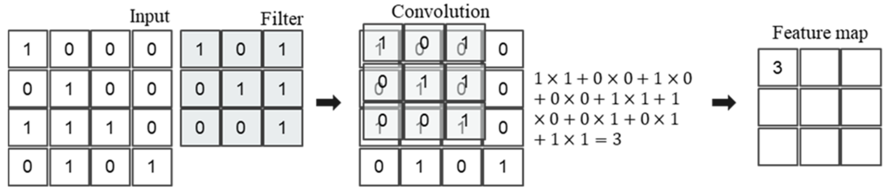
Figure 1 shows the output when the convolution operation is performed using a 3 × 3 filter on the 4 × 4 input data. The filters used shared weights and were continuously updated to determine the optimal value while training the model.
2.2. Pooling Layer
Pooling is the process of sub-sampling the results of the convolution layer. Similar to a convolution layer, a filter with a specific size and stride is used to extract the maximum value, called max pooling, or the average value, called average pooling. In a CNN, the number of parameters to learn increases rapidly as the layers become deeper. In such cases, the input size can be reduced through pooling, and overfitting can be avoided by reducing the number of training parameters.
2.3. Normalization
Batch normalization [
15] appeared to solve problems, such as gradient vanishing, in which the gradient disappears during back-propagation. Problems such as gradient vanishing can occur owing to the internal covariance shift, which is caused by different distributions of inputs to each layer of the network. To prevent this phenomenon, a method of normalizing the input was used, for which batch norm, layer norm [
16], instance norm [
17], and group norm [
18] exist. Because we used input data with a large image size and a large number of channels, we adopted the group norm and reduced the batch size.
2.4. Dense-UNet
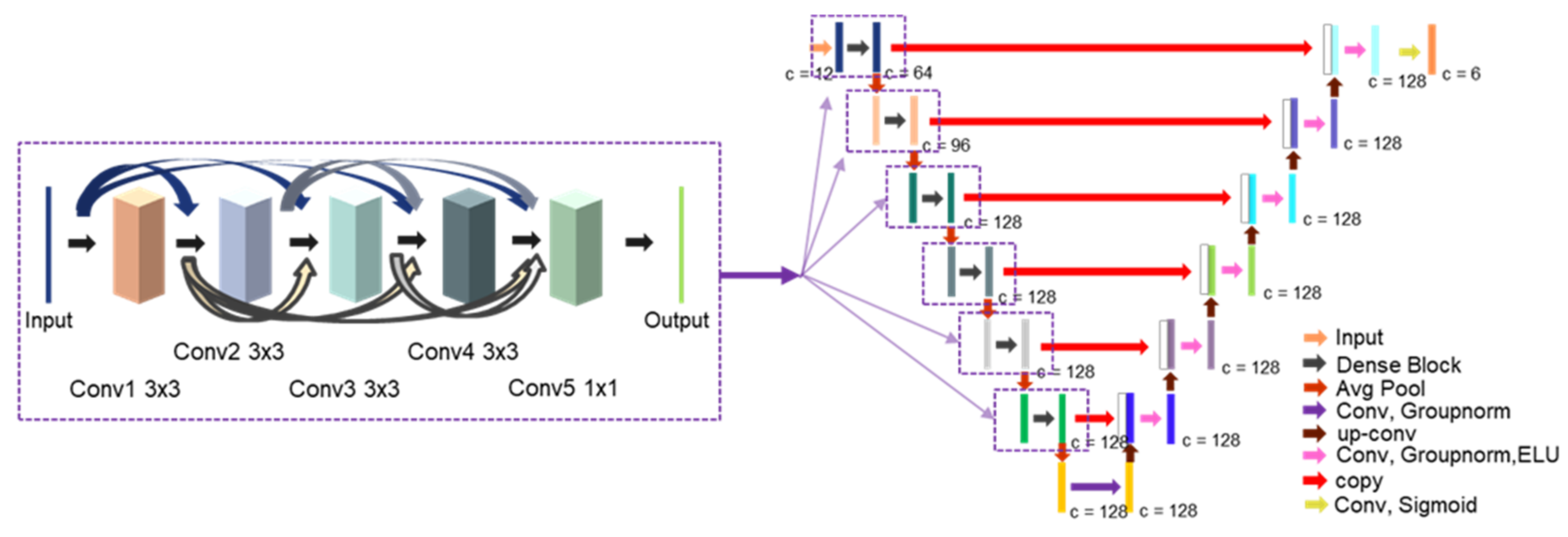
UNet is a U-shaped model used in image. Image segmentation does not simply classify an image, but refers to labeling specific pixel regions of an image. UNet has attracted attention because it performs accurate segmentation using a small amount of medical data. In particular, UNet solves the trade-off problem of not being able to grasp the context of understanding a wide range of images and detailed localization at once. The UNet consists of a contracting path on the left side and an expanding path on the right side around the bottleneck in the middle. The contracting path creates a feature map and identifies the context of image pixels. The expanding path segments the object by combining the image context and up-convolution output. As shown in
Figure 2, we used a densely connected UNet, which is a UNet model with densely connected convolution layers of the contracting path [
19], called Dense-UNet. The input and output of the convolution layer were combined and used as the input for all the other convolution layers.
3. Proposed Method
3.1. Framework
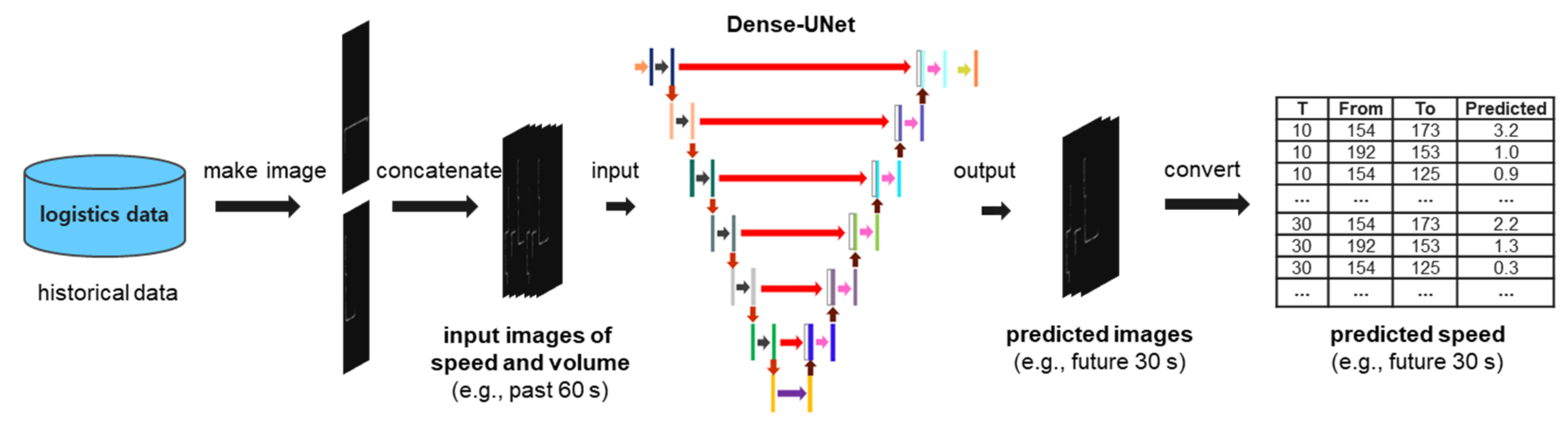
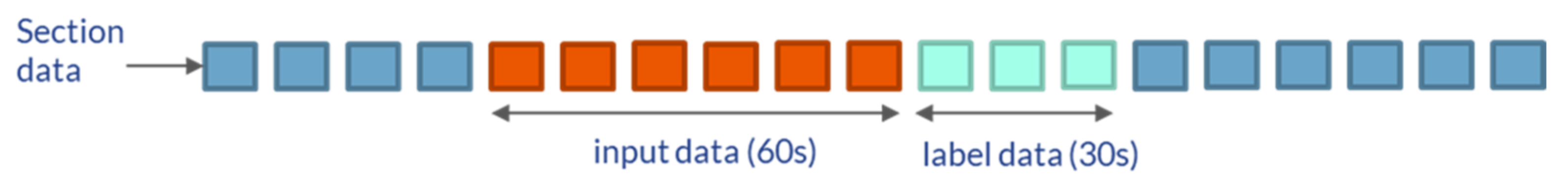
We obtained logistic data at 10 s intervals from the simulator. These logistic data were imaged one by one. When creating an image, the input volume and speed information are obtained using the coordinate information for each section in a 2D array. By concatenating the image created in this manner into channels by a certain window size, we obtain the input of the learning model. Additionally, we needed a label to be used when training the model. These labels used future images. As with input data, it is possible to consider future information for a specific time by concatenating it into channels of a specific window size. In our experiment, we addressed the problem of predicting 30 s into the future using data from the past 60 s. The model was trained using input and label data collected in this manner. When the model is trained, it outputs an image containing the prediction value of the future 30 s for the input. Finally, to compare our logistic data with the predicted value, we converted the predicted image back to the logistic data. Through this process, the learning result can be obtained with the volume and speed information in the fab, and a visualization of all these processes is shown in
Figure 3.
3.2. Encoding Logistic Data to Traffic Image
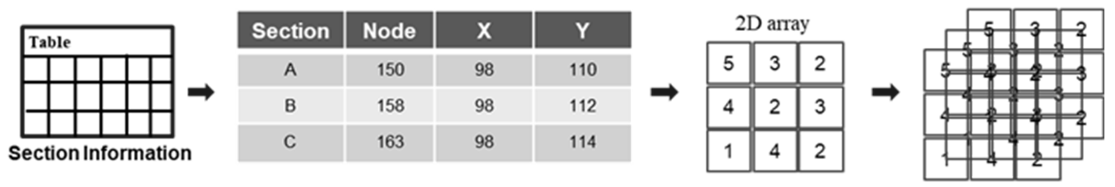
Here, the process of converting logistic data into image data is described in detail. Because we know the coordinate values of all the sections, we can map the volume and velocity information of each section to specific coordinate values in a 2D array, as shown in
Figure 4. However, if the size of the image becomes too large, it is difficult to use it as an input to the model; therefore, there are cases where pure coordinate information cannot be used as it is. Consequently, the coordinate information is mapped to a 2D array using a value divided according to the image size. At this time, the volume and speed values are converted to values between 0 and 255 for mapping, and the maximum volume and speed used according to the data are set and used. Because one piece of logistic data has two pieces of information, volume and speed, two images can be obtained from one piece of logistic data: a volume image and a speed image. As shown in
Figure 5, by concatenating the created images one by one on a channel basis, it creates input data, which considers past information up to a specific time and creates label data, which considers future information up to a specific time.
3.3. Decoding Traffic Image to Logistic Data
From the trained model, we obtained a predicted image for the future. As the output image is grouped by the channel standard, it is used to obtain the predicted value by dividing it by the channel standard. In the encoding process, two images were obtained with one logistic dataset; however, in the decoding process, one logistic dataset was created from two output images. The volume and speed values were mapped to a 2D array using specific coordinate values during the encoding process. Inverse transformation was performed again using the maximum volume and speed used in the mapping process. First, the average value of the pixels between the two is calculated based on the start and end nodes of one section. The average pixel value obtained in this manner is inversely transformed into volume and speed and is used as a prediction value.
4. Experiments
4.1. OHT Traffic Data
The data used in the experiments were simulated data based on the actual semiconductor factory data. The semiconductor factory consists of several floors and buildings; however, we analyzed data from only one floor. It is composed of thousands of nodes, and the connection of nodes is called “link,” and the connection of several “links” is called a “section”. We created one image for thousands of sections and proceeded with the learning. In the 10 s interval data, 24 h were used as training data, the other 6 h were used as validation data, and another 6 h were used as test data.
4.2. Encoding Traffic Data to Traffic Image
We trained the model by creating images of the past 60 s of data as the input data. The volume or speed information was mapped onto one image channel. When mapping information to an image, using the actual coordinate value creates an unusable image size; therefore, the actual coordinate value is divided by 1000 and then used. Two pieces of information, volume and speed, can be found in the data at 10 s intervals. In other words, the input data had 2 × 6 = 12 channels, and the image size was (512, 256) considering the coordinates of the sections. For training data, 24 h × 60 min × 6 − 3 (last window of data) = 8637 images were created, and 6 × 60 × 6 − 3 (last window of data) = 2157 images for validation and test data were created.
The output shape of each layer is listed in
Table 1.
B in the output shape indicates the batch size. The size of the first input image was (512, 256). In the contracting path, the channel size increases and the image size decreases. The image size increases again through the expanding path, and the size of the final output image becomes the same as that of the input image.
4.3. CNN Based Prediction Model for Traffic Image
When training our model, the shape of the first input image was (12, 512, 256). In the contracting path, the number of channels increases and the image size decreases as it passes through the dense block and pooling layer. If it passes through six dense blocks and a pooling layer, the output shape becomes (128, 8, 4). The output of the contracting path passes through one convolution layer, and then through an expanding path. In the expanding path, the size of the image is increased again through the convolution transpose layer, which works in a manner opposite to the convolution layer. The output shape that has passed through the six convolution transpose layers becomes (128, 512, 256), and the final output of the shape (6, 512, 256) is the output through the last convolution layer and activation function. The output shapes passing through several layers are summarized in
Table 1.
4.4. Decoding Traffic Image to Traffic Data
Because we predict the future 30 s at 10 s intervals, our model outputs six channels with volume and speed as channels. Each channel represents a volume and speed of 10 s, 20 s, and 30 s in the future. Because we know the location information of each section used in the encoding, we can read the pixel value of the required section from the predicted image. Only the pixel values between the start and end positions of the section are averaged and used as the pixel values for the section. After obtaining the average pixel value of each section, the prediction speed value is obtained through an inverse transformation process of mapping to the image.
4.5. Experimental Results
We compared the experimental results with the following four models:
Historical average (HA) model: The overall average speed of the train data is used as a predicted value;
Rct60s model: The average speed from the current time point t to the past 60 s is used as the predicted value;
Rct30s model: The average speed from the current time point t to the past 30 s is used as the predicted value;
Rct10s model: The average speed from the current time point t to the past 10 s is used as the predicted value.
Root mean square error (RMSE), mean absolute error (MAE) and coefficient of determination (
R2) are used as evaluation indicators. To predict the near future, we divide the time interval into 10 s, 20 s and 30 s to predict the future average speed.
Table 2 shows the experimental results for each time interval
T. The experiment was conducted in a PyTorch environment using Intel Xeon Silver 4210 CPU and Nvidia Titan RTX 24 GB.
As shown in
Table 2, the MAE of the average speed prediction of 10 s, 20 s, and 30 s in the future is the smallest value when using Dense-UNet. In contrast, RMSE and
R2 yielded the best results for the HA model. In the case of a large error, the performance of the HA model is better; however, the absolute difference between the actual value and the predicted value shows that Dense-UNet has a better prediction performance. It can be observed that the error tends to increase as the time interval T increases. It has been confirmed that it predicts the near time more accurately; it becomes more difficult to predict further into the future.
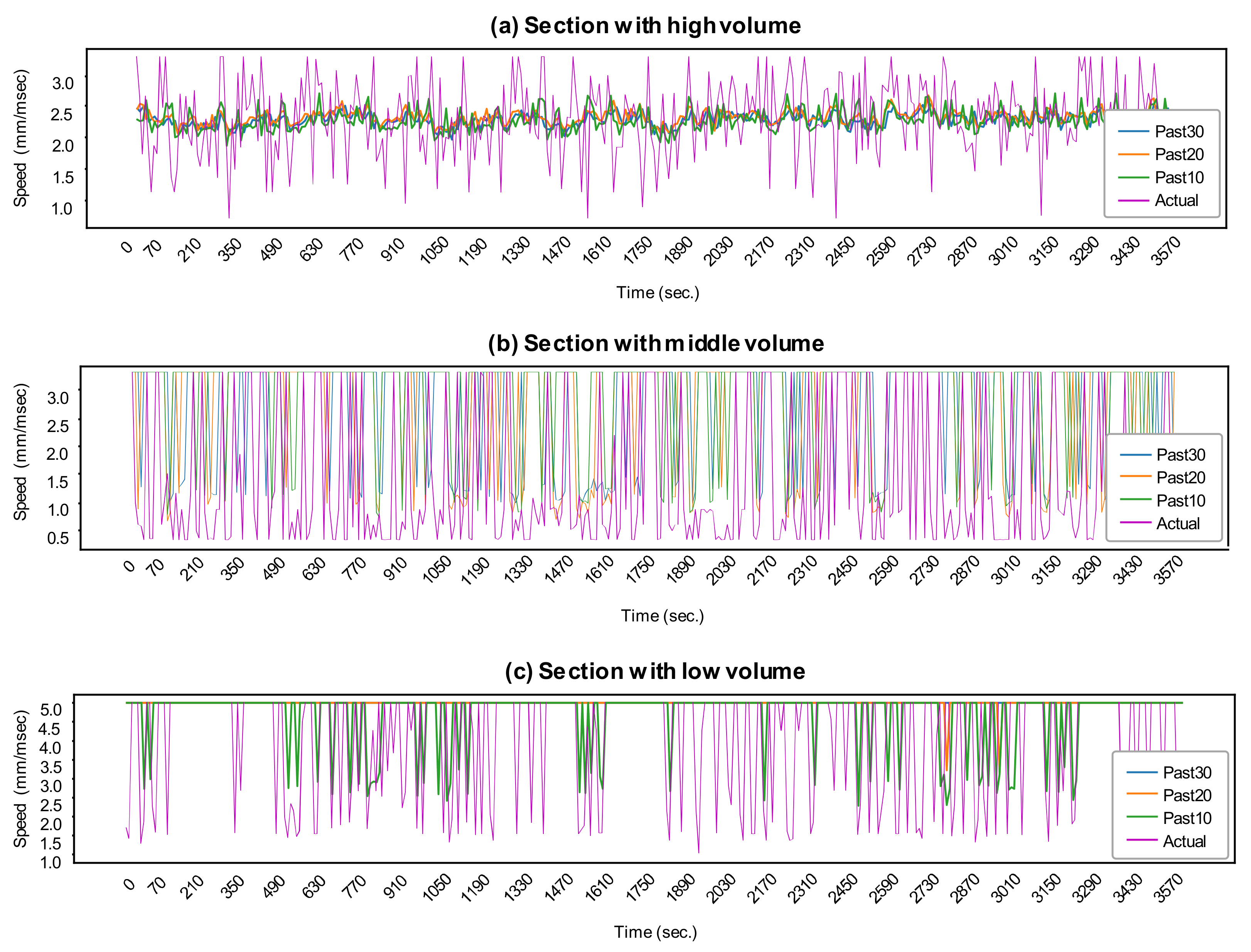
The average volume of each section differed. The change in the average speed prediction according to the average volume can be expressed as a time series graph, as shown in
Figure 6.
Figure 6a shows a section with a high volume of traffic,
Figure 6b shows a section with medium volume, and
Figure 6c shows a section with low volume.
In the case of high traffic volume, the change in average speed appears very rapidly in a short time. In this case, the predicted value follows the trend of the average speed change but does not show a large change in value. In the case of medium volume, the speed decreases momentarily and then returns to the standard speed. In this case, it can be confirmed that the predicted value follows the trend and exhibits a large change in value. It can be observed that changes in the average speed occur occasionally when the volume of traffic is small, and in this case, it was confirmed that the predicted value partially followed the instantaneous fall.
5. Conclusions and Future Work
In this study, we dealt with the time series problem through the segmentation technique Dense-UNet. Unlike previous studies that have generated and utilized many features for time series prediction, this study used only the most basic average volume and average speed information. In addition, to understand the flow in the fab, we present a method for training the model by converting the information into an image.
For the future 10 s, 20 s, and 30 s predictions, Dense-UNet showed the best results for MAE, and the HA model was good in terms of RMSE and R2. Additionally, we examined the time series graph according to the volume, and it was confirmed that the predicted values changed effectively for the sections with a medium volume.
Although only the basic information of each section was used, it is expected that design information, such as section length, can be used in future studies. In addition, because it is not very efficient to use a complex model to predict the sections with a very low traffic volume, it is expected that it will be possible to train the model by selecting only the sections with a high traffic volume and creating a smaller image.
Author Contributions
Conceptualization, Y.H.J., H.K. and J.-Y.J.; methodology, Y.H.J. and J.-Y.J.; software, Y.H.J.; validation, H.P., H.K., R.C., Y.K. and J.-Y.J.; data curation, Y.K. and R.C.; writing—original draft preparation, Y.H.J.; writing—review and editing, H.P. and J.-Y.J.; visualization, Y.H.J. and J.-Y.J.; supervision, J.-Y.J.; project administration, J.-Y.J.; funding acquisition, J.-Y.J. All authors have read and agreed to the published version of the manuscript.
Funding
This study was conducted with the support of Samsung Electronics (IO200423-07296-01). In addition, this work was partially supported by the Korea Institute for Advancement of Technology (KIAT) grant funded by the Korea Government (MOTIE, Korea) (Advanced Training Program for Smart Factory, No. N0002429) and the BK21 FOUR (Fostering Outstanding Universities for Research) funded by the Ministry of Education (MOE, Korea) and National Research Foundation of Korea (NRF).
Institutional Review Board Statement
Not applicable.
Informed Consent Statement
Not applicable.
Conflicts of Interest
The authors declare no conflict of interest.
References
- Zhou, Q.; Zhou, B.H. An impending deadlock-free scheduling method in the case of unified automated material handling systems in 300 mm wafer fabrications. J. Intell. Manuf. 2018, 29, 155–164. [Google Scholar] [CrossRef]
- Liao, D.Y.; Fu, H.S. Speedy delivery-dynamic OHT allocation and dispatching in large-scale, 300-mm AMHS management. IEEE Robot. Autom. Mag. 2004, 11, 22–32. [Google Scholar]
- Kim, B.I.; Shin, J.; Jeong, S.; Koo, J. Effective overhead hoist transport dispatching based on the Hungarian algorithm for a large semiconductor FAB. Int. J. Prod. Res. 2009, 47, 2823–2834. [Google Scholar] [CrossRef]
- Sakr, A.H.; Aboelhassan, A.; Yacout, S.; Bassetto, S. Simulation and deep reinforcement learning for adaptive dispatching in semiconductor manufacturing systems. J. Intell. Manuf. 2021, 1–14. [Google Scholar] [CrossRef]
- Bartlett, K.; Lee, J.; Ahmed, S.; Nemhauser, G.; Sokol, J.; Na, B. Congestion-aware dynamic routing in automated material handling systems. Comput. Ind. Eng. 2014, 70, 176–182. [Google Scholar] [CrossRef]
- Nakamura, R.; Sawada, K.; Shin, S.; Kumagai, K.; Yoneda, H. Model reformulation for conflict-free routing problems using Petri net and deterministic finite automaton. Artif. Life Robot. 2015, 20, 262–269. [Google Scholar] [CrossRef]
- Hwang, I.; Jang, Y.J. Q(λ) learning-based dynamic route guidance algorithm for overhead hoist transport systems in semiconductor fabs. Int. J. Prod. Res. 2020, 58, 1199–1221. [Google Scholar] [CrossRef]
- Ahn, K.; Lee, K.; Yeon, J.; Park, J. Congestion-aware dynamic routing for an overhead hoist transporter system using a graph convolutional gated recurrent unit. IISE Trans. 2022, 54, 803–816. [Google Scholar]
- Kim, H.J.; Lee, J.H.; Baik, S.; Lee, T.E. Scheduling in-line multiple cluster tools. IEEE Trans. Semicond. Manuf. 2015, 28, 171–179. [Google Scholar]
- Wan, J.; Shin, H. Predictive vehicle dispatching method for overhead hoist transport systems in semiconductor fabs. Int. J. Prod. Res. 2022, 60, 3063–3077. [Google Scholar] [CrossRef]
- Lingitz, L.; Gallina, V.; Ansari, F.; Gyulai, D.; Pfeiffer, A.; Sihn, W.; Monostori, L. Lead time prediction using machine learning algorithms: A case study by a semiconductor manufacturer. Procedia CIRP 2018, 72, 1051–1056. [Google Scholar] [CrossRef]
- Wang, J.; Yang, J.; Zhang, J.; Wang, X.; Zhang, W. Big data driven cycle time parallel prediction for production planning in wafer manufacturing. Enterp. Inf. Syst. 2018, 12, 714–732. [Google Scholar] [CrossRef]
- Ronneberger, O.; Fischer, P.; Brox, T. U-net: Convolutional networks for biomedical image segmentation. In Proceedings of the International Conference on Medical Image Computing and Computer-assisted Intervention, Munich, Germany, 5–9 October 2015. [Google Scholar]
- Clevert, D.A.; Unterthiner, T.; Hochreiter, S. Fast and accurate deep network learning by exponential linear units (elus). arXiv, 2015; arXiv:1511.07289. [Google Scholar]
- Ioffe, S.; Szegedy, C. Batch normalization: Accelerating deep network training by reducing internal covariate shift. In Proceedings of the International Conference on Machine Learning, Lille, France, 6–11 June 2015. [Google Scholar]
- Ba, J.L.; Kiros, J.R.; Hinton, G.E. Layer normalization. arXiv, 2016; arXiv:1607.06450. [Google Scholar]
- Ulyanov, D.; Vedaldi, A.; Lempitsky, V. Instance normalization: The missing ingredient for fast stylization. arXiv, 2016; arXiv:1607.08022. [Google Scholar]
- Huang, G.; Liu, Z.; Van Der Maaten, L.; Weinberger, K.Q. Densely connected convolutional networks. In Proceedings of the IEEE Conference on Computer Vision and Pattern Recognition, Honolulu, HI, USA, 21–26 July 2017. [Google Scholar]
- Wu, Y.; He, K. Group normalization. In Proceedings of the European Conference on Computer Vision, Munich, Germany, 8–14 September 2018. [Google Scholar]
| Publisher’s Note: MDPI stays neutral with regard to jurisdictional claims in published maps and institutional affiliations. |
© 2022 by the authors. Licensee MDPI, Basel, Switzerland. This article is an open access article distributed under the terms and conditions of the Creative Commons Attribution (CC BY) license (https://creativecommons.org/licenses/by/4.0/).


 ,
, 


