Model Prediction and Optimization of Waste Lube Oil Treated with Natural Clay

Abstract

In this work, used lube oil was treated using natural acid-free clay. Clay was added at different amounts (5, 10, and 20 g) to 100 mL of waste engine oil at various temperatures (250, 350, 400, and 450 °C) and mixed at a speed of 800 rpm for 30 min. After settling and separation, the treated oil was diluted with kerosene before being examined using a Ultraviolet–visible (UV) spectrophotometer. In order to achieve cost-effective recycling, this process is modeled using the response surface method (RSM). Five regression models (linear, quadratic, Two Factor Interactions (2FI), cubic, and reduced-order quadratic model) were developed, then tested, and examined by calculating the statistical performance indicators (R², R²_adj, Akaike’s Information Criterion corrected (AICc), Bayesian Information Criterion (BIC), and Root Mean Square Error (RMSE)). The results obtained reveal that the modified quadratic model outperforms the rest of the models in terms of the low value of RMSE, the lowest AICc, lowest BIC, and the highest R² and R²_adj. The developed modified quadratic model is optimized successfully to predict optimum operation conditions. Results show that optimum operation conditions are at the minimum area under the curve for UV absorption at 223.358; this can be achieved with a process temperature of 266.246 °C and clay quantity of 5.331 g. This model agreed with experimental data regardless of the effectiveness of red clay in the therapy of lube oil.

1. Introduction

Lubricants generated by the crude oil refining sector denote approximately 1.2% of annual petroleum consumption. At a worldwide level, this value corresponds to more than 40 million tonnes of base oil [1]. Refining of crude oil produces about 67% of base lube oil while recycling of used oil can produce up to 95% of base oil. These lubricating oils mainly consist of complicated mixtures of isoalkanes with slightly longer branches, and with monocycloalkanes and monoaramatics having several short branches on the ring [2]. The chemical structure of the lubricating oil differs considerably depending on the kinds and percentages of additives; these are also dependent on the applications of the oil [3].

During application, lubricating oils tend to degrade leading to the deterioration of various important features, such as rheological and film-forming properties. Rheological properties are considered to be among the most important degradable properties [4]. Waste lubricant oil disposal causes serious environmental damage [5]. Unburned lubricating oil was found to have a high contribution to particulate emissions [6]. Therefore, waste engine oil has gained significant attention from researchers for a long time, which has resulted in various methods for the treatment and recovery of base oil being developed. Over the years, the removal of waste lubricating oil contaminants using solvents has been studied [7,8,9,10,11]; the use of clay as a bleaching agent, especially bentonite, has been mentioned in the literature [12].

Traditional treatment with clay-acid utilizes concentrated sulfuric acid to remove asphalt compounds and generates highly toxic acid products. Waste oils are originally handled with natural polymers to remove carbonic elements in the regeneration technique using acid-free clays. The oil is then subjected to vacuum distillation and clay treatment in an appropriate amount to accomplish the necessary product coloration [13,14]. In addition to the high expense due to the amount of clay needed, the recovered oils obtained through this process still have relatively high metal percentages [15]. The use of activated carbon has also been reported in the literature and the results showed a highly effective waste engine oil treatment by polycyclic aromatic hydrocarbon (PAH) removal [16]. Process optimization and oil property improvement achieved through acid modification of clays is now generating a renewed interest by researchers in recycling waste engine oil [17,18].

In this paper, the quality of the obtained oil after clay treatment at various conditions is assessed using UV spectrophotometer. The variation in light intensity due to absorption is determined by the amount of absorbance, according to the Beer–Lambert relationship. The Beer–Lambert relationship says that there is a logarithmic dependency between the transmission of light through a substance and the product of the substance’s absorption coefficient and the distance the light passes or travels through the material i.e., the length of the route “l.”

$$A=-logT=log\frac{I_0}{I}=a·c·b$$

(1)

where A is the absorbance, T is the transmission defined as I/I₀, I is the incident luminance, Io is the transmitted luminous intensity, a is the absorbing type absorbance, c is the absorbing type concentration (g/L), and b is the trajectory length of the luminous. The chemicals dissolved in oil can be characterized by the transmission of certain wavelengths to a compound and by the measurement of light intensity [19].

In the process industry, if high efficiency is to be achieved, the most advanced process control system needs precise models. Most chemical processes are nonlinear in nature, making the development of precise models difficult [20,21]. Different factors, ranging from model nonlinearity to dimensionality and the data sampling method to internal parameters are considerably influenced when examining the accuracy of the modeling technique [22].

The scope of this paper is to develop a prediction model for (Ultraviolet–visible) (UV-VIS) spectrophotometer data for the lube oil treatment process, which can play an important role in optimizing process operating conditions. A model capable of predicting experimental behavior correctly has been pursued earnestly by various researchers over the years.

In many engineering aspects, such models can dramatically decrease time and operating costs. The need for modeling the used lube recycling process using red clay under various operating conditions emerged from the above mentioned reasons. The response surface models are among the most recognized modeling techniques that are used widely [22,23,24,25,26,27]. Extensive surveys and reviews of various modeling techniques and their applications are provided by [28,29,30,31].

2. Methodology

2.1. Experimental Methods

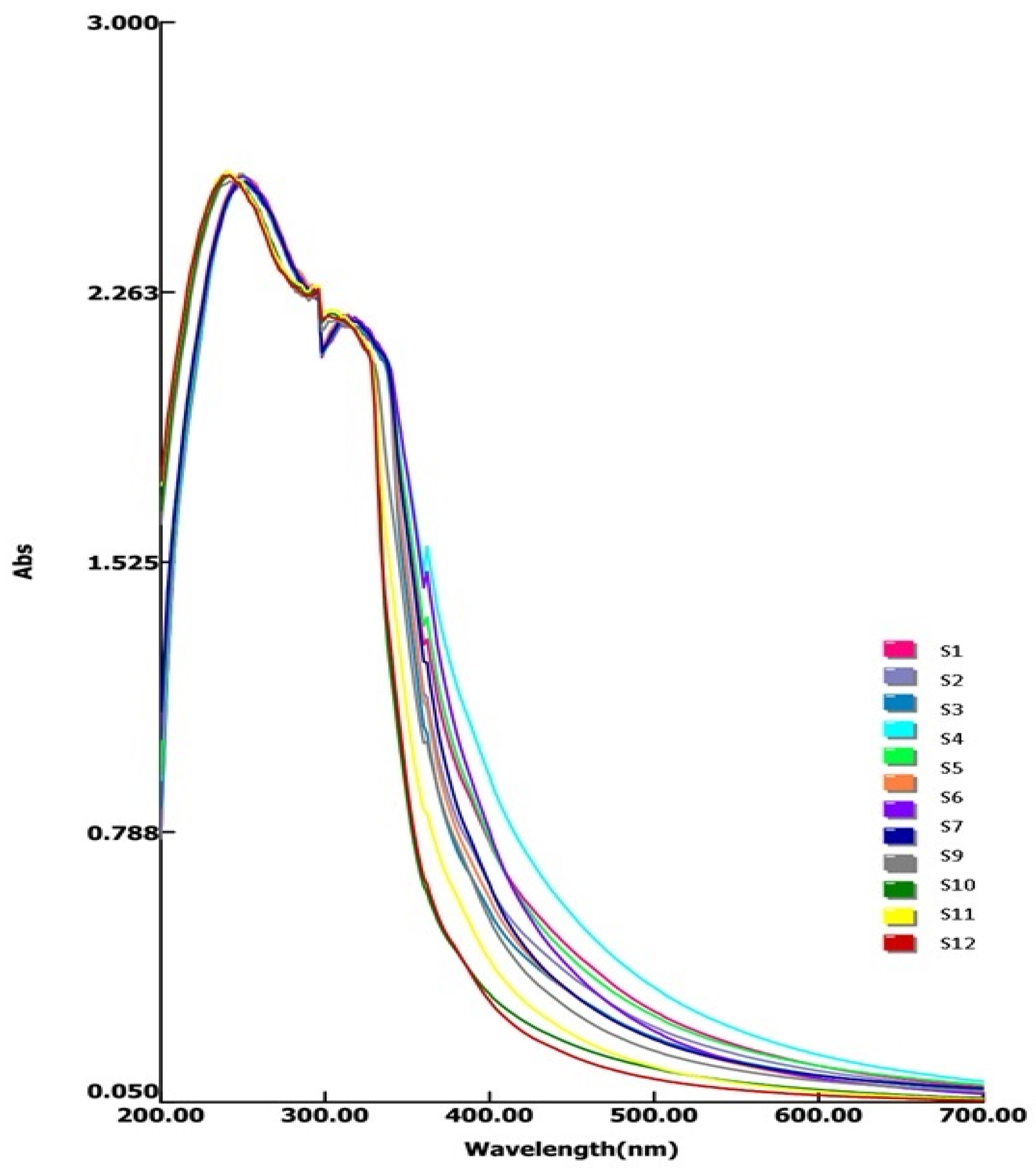
Fresh SAE (Society of Automotive Engineers) 20W-50 oil was introduced into an automotive engine, which was then operated for 3500 km. The used oil was subsequently collected for treatment and evaluation. Three liters were filtered and left for 48 h after and all settled particles were removed. Then the natural red clay was washed with distilled water, dried, and then crushed and sieved with a 200 µm mesh. Different quantities of clay (5, 10, and 20 g) was added to 100 mL of the waste engine oil. Each set of flasks containing oil-clay mixture was then subjected to specific temperatures: 100, 250, 350, and 450 °C with a constant mixing speed of 800 rpm for 3 h according to the method reported in [32]. The mixtures were then left to cool naturally to room temperature and to allow the clay to settle. Simple decantation was used to obtain most of the oil before the use of filtration. Samples from the treated oil (4 mL) were then diluted using kerosene (1 L) before being tested using a UV spectrophotometer. Kerosene was chosen because it is more suitable to mass spectrometric analysis as reported in [33]. The UV results are shown in Figure 1; the complexity of the graph emerged to show an effective way to optimize the operating conditions, which gave the best treatment.

Summary of UV spectrophotometer results is presented in

Table 1. Absorbance area under the curve of the different samples.

Sample	Temperature °C	Concentration g/100 mL	Abs. Area Under Curve from 200–300 nm
S1	250	5	224.66
S2	250	10	224.08
S3	250	20	225.21
S4	350	5	226.89
S5	350	10	227.51
S6	350	20	229.4
S7	400	5	228.39
S8	400	10	228.32
S9	400	20	235.62
S10	450	5	237.52
S11	450	10	239.38
S12	450	20	238.56

. A range of wavelengths from 200 to 350 nm was defined and the area under the curve was noted for all the twelve tested samples.

2.2. Modeling Techniques

Multiple regression models were used in this study based on the response surface method: (a) linnear model, (b) 2 FI model, (c) quadratic model, (d) cubic model, (e) reduced term quadratic model.

Response Surface Methodology (RSM)

The response surface methodology came from the original work [23]. Their cooperation began when solving the issue of determining optimum operating conditions for a particular chemical process. The methodology of the response surface is used in many practical applications where the goal is to identify the levels of design factors or variables that optimize a response. Despite its simplicity and efficiency, RSM provides efficient and accurate solutions. It has therefore been applied effectively to many engineering aspects [34,35,36,37].

Before implementing the RSM methodology, it is first essential to select an experimental design to define which runs should be conducted in the studied experimental range [38].

For this purpose, there are some experimental matrices. Experimental designs can be used for first-order models (e.g., factorial designs) if there is no curvature in the data set [38]. However, in order to approximate a response function to experimental data which cannot be characterized by linear functions, experimental designs for quadratic response surfaces, such as three-level factorial models, Box–Behnken, central composite, and Doehlert designs should be used [39].

In this study, a three-level full factorial design is applied, the minimum number of experiments required for this design can be calculated by the expression N = 3^k, where N is the number of experiments and k is the independent variable. Other designs, such as the Box–Behnken and central composite design (CCD) are used more frequently for more than two factors because the full factorial design needs more experimental runs than can normally be accommodated in practice [39].

RSM is a higher-order polynomial that determines a best-fit polynomial of desired order developed after applying an ANalysis Of VAriance ANOVA test to express the value of the variable Y (lube oil absorbance, in this case) as a function of the independent variables (X1 and X2) as follows [27]:

$$\mathrm{Y}={\beta }_o+{\displaystyle \sum }_{i=1}^2{\beta }_i{X}_i+{\displaystyle \sum }_{i=1}^2{\beta }_{ii}{X}_i^2+{{\displaystyle \sum }}_{j=1}^2{{\displaystyle \sum }}_{i<j=1}^2{\beta }_{ii}{X}_i{X}_j$$

(2)

where β₀, β_i, and β _ii, are the regression intercept constants and the notations X₁ = A and X₂ = B are the independent variables, as shown in

Table 2. Experimental design variables used for modeling the absorbance of treated lube oil.

Independent Variables Xn	Coded Levels
	−1	0	1
X1: Temperature (°C) A	250	362.5	450
X2: Concentration (g/L) B	5	11.66	20

.

2.3. Model Validation and Evaluation

R² and error analyses were performed between the experimental and predicted data in the four models to evaluate the goodness of the model fitting and prediction accuracy of the constructed models. Many approaches for validation are stated in the literature are used for error analyses, some are listed in [40].

In this paper, promising techniques that used the error as performance indices to measure the model accuracy are introduced. There are a number of different measures of model accuracy. The first two are the root mean square error (RMSE) and the R² values.

In general, the larger the values of R² and R²_adj, and the smaller the value of RMSE, the better the fit. It is more appropriate to look at R²_adj in situations where the number of design variables is large because R² always increases as the number of terms in the model increases, while R²_adj actually decreases if unnecessary terms are added to the model. Different techniques for statistical analysis i.e., ANOVA test can be used to check an RSM model’s fitness, thus identifying the main effects of the design variables. The major statistical parameters used for evaluating model fitness are the F statistic, R, adjusted R², and the root mean square error (RMSE) [27,41].

These parameters are not totally independent of each other and are calculated by:

2.3.1. Root Mean Square Error (RMSE)

In general terms, the lower the RMSE value, the better the fit. It could be calculated as:

$$RMSE=\sqrt{\frac{SSE}{n-p-1}}$$

(3)

where p is the number of non-constant terms in the RSM model, SSE is the sum square error, and SST is the total sum square. The calculations for SSE and SST are:

$$SSE={\displaystyle \sum }_{i=1}^n{\left(fi-f^{\prime }\right)}^2$$

(4)

$$SST={\displaystyle \sum }_{i=1}^n{\left(fi-\overline{f}\right)}^2$$

(5)

where fi is the measured function value at the i-th design point, f_i is the calculated function value from the I design point of the polynomial and f is the mean value of f_i.

2.3.2. R², R²_adj, and R²_pred

In situations where the number of design variables is large, it is more appropriate to look at R²_adj because R² always increases as the number of terms in the model increases:

$$R^2=1-\frac{SSE}{SST}$$

(6)

In fact, R²_adj reduces if the model is added to unnecessary terms:

$$R_{adj}^2=1-\left(1-\mathrm{R}\right)\frac{\mathrm{n}-1}{n-p-1}$$

(7)

R²_pred is a measure of the percentage of variation described by the model in new data:

$$R_{pred}^2=1-\frac{PRESS}{SST}$$

(8)

where Predicted Residual Error Sum of Squares PRESS is a measure of how each point in the design fit the mode:

$$PRESS={{\displaystyle \sum }}_{i=1}^n\left(e_{-i}\right)$$

(9)

e_–i is a deletion residual computed by fitting a model without the i-th run then trying to predict the i-th observation with the resulting model.

The adjusted R-squared and the predicted R-squared should be within 0.20 of each other.

2.3.3. AIC and BIC

AIC stands for Akaike’s information criterion for a small design. It is commonly used for validity measurement within a cohort of nonlinear models and is often used for model selection. It is calculated as follows:

AIC = 2p − 2ln(L)

(10)

where p = number of parameters and ln(L) = maximum log-likelihood of the estimated model. The latter, in the case of a nonlinear fit with normally distributed errors [42]. This is calculated by:

$$ln\left(L\right)=0.5\left(-N\left(ln2\pi +1-lnN+ln{\displaystyle \sum }_{i=1}^n{x}_i^2\right)\right)$$

(11)

where x₁, …, x_n are the residuals from the nonlinear least-square fit and N = their number

For small sample sizes, AIC tends to choose models that have too many terms. The AIC corrected (AICc) is used to overcome these issues by increasing the penalty on additional terms for smaller designs.

$$AICc=AIC+\frac{2p\left(p=1\right)}{n-p-1}$$

(12)

where n = sample size and p = number of parameters.

Bayesian information criterion (BIC)

BIC is an alternate to AICc that performs better for larger designs. It is calculated by:

BIC = p ln (n) − 2 ln (L)

(13)

where p is the number of parameters, n = sample size, and L = maximum likelihood of the estimated model.

2.3.4. Modeling Statistics

To compare predictive model terms several statistical indices can be used but are not limited to:

RMSE: Square root of the residual mean square. Consider this to be an estimate of the standard deviation associated with the experiment.

Mean: Overall average of all the response data.

C.V.: (coefficient of variation) the standard deviation expressed as a percentage of the mean. It can be calculated by dividing the standard deviation by the mean and multiplying by 100.

PRESS: (predicted residual error sum of squares) A measure of how the model fits each design point.

Adequate accuracy: this is the ratio of signal to noise. It compares the range of predicted values at the design points with the average error of prediction. Ratios larger than 4 indicate adequate discrimination in the model.

3. Results and Discussion

The UV absorbance values for the treated oil (S1–S12) differ substantially over a broad spectrum of wavelengths, a comparative absorbance assessment is shown in Figure 1. This is due to the presence of very complex mixtures of paraffinic, naphthenic, and aromatic hydrocarbon molecules in addition to waste material [9]. As the kerosene is introduced to dilute samples, the viscosity of oil samples becomes less. Consequently, the sample oil becomes optically more transparent. The UV spectrometer data is modeled to optimize the process operation parameters

The model prediction is created using Design Expert 10 on Windows 7 with i5 8 Gigabite (GB) of Read Access Memory (RAM) to assess the computational effectiveness and precision of the models developed; the above performance evaluation features are recognized as excellent indices. The large values of R²_adj and R², as well as small values of RMSE, indicate good fitting for the models.

3.1. Modeling Experimental Data Using RSM

Five models were compared together: linear model, quadratic model, cubic model, and Two Factor Interactions Model (2FI model).

3.1.1. Linear Model

When applying the developed model using the previously defined data, the following pre-model has been obtained and the final equation in terms of actual factors is as follows:

Absorption area under the curve = +204.98717 + 0.063973 × Temperature +0.19579 × Concentration

Regression coefficients and statistical analysis for the predicted response surface model are shown in

Table 3. Linear model regression coefficients statistical analysis.

Factor	Coefficient Estimate	Df	Standard Error	95% CI Low	95% CI High	F-Value	P-Value
MODEL						18.81	0.0006	significant
Intercept	229.83	1	0.81	227.98	231.67		--	---
A-Temperature	6.40	1	1.08	3.96	8.83	35.28	0.0002
B-Concentration	1.47	1	0.96	−0.70	3.64	2.35	0.1597

.

It was observed that the calculated F-value of 18.81 from Table 3 indicates that the model is significant (as it is desirable to have the biggest value). However, to specify that model terms are significant, the P-value should be less than 0.05. Only the A-temperature is regarded as a significant model term in this situation.

The model was verified using the statistical test ANOVA in which

Table 4. Analysis of statistical variance.

RMSE	2.76	R2	0.8070
Mean	230.46	R2adj dj	0.7641
C.V.%	1.20	R2pred	0.6808
PRESS	113.33	Adeq Precision	11.402
		BIC	62.42
		AICc	63.96

was acquired.

The 0.6808 “R²_pred” is, to be exact, in significant agreement with the 0.7641 “R²_adj;” the difference is less than 0.2. The “Adeq Precision” measures the ratio of signal to noise. It is desirable to have a ratio higher than 4; 11.402 shows an appropriate signal ratio in this situation. However, the search emerges for another better model with insignificant terms.

3.1.2. The Quadratic Model

The final equation model in terms of coded factors is presented in the following quadratic form:

Abs. area under the curve = +227.03 + 6.76 × A + 1.35 × B + 0.55 × AB + 4.19 × A² + 0.55 + B²

As can be seen from

Table 5. Quadratic model regression coefficients statistical analysis.

Factor	Coefficient Estimate	Df	Standard Error	95% CI Low	95% CI High	F-Value	P-Value
MODEL						15.73	0.0022
Intercept	227.03	1	1.41	223.57	230.49	69.24
A-Temperature	6.76	1	0.81	4.77	8.75	3.37	0.0002
B-Concentration	1.35	1	0.73	−0.45	3.14	0.33	0.1161
AB	0.55	1	0.96	−1.80	2.90	9.86	0.5868
A2	4.19	1	1.33	0.93	7.45	0.15	0.0200
B2	0.55	1	1.44	-2.97	4.06	15.73	0.7163

, only two terms of temperature and temperature² are significant in this quadratic model (p-value less than 0.05).

Table 6. Analysis of statistical variance.

RMSE	2.05	R2	0.9291
Mean	230.46	R2adj	0.8700
C.V.%	0.89	R2pred	0.6980
		Adeq Precision	11.195
		BIC	57.85
		AICc	71.74

displays the 0.6980 “R²_pred” insensible agreement with the 0.8700 “R²_adj”. On the other hand, “Adeq Precision” measures the signal-to-noise ratio where it is desirable to have a ratio greater than 4. The 11.195 model ratio stated an appropriate signal as the difference is lower than 0.2, which is lower than the pre-model. In addition, the F value of 15.73 is also less than the prior one. This model may be enhanced.

Only the temperature conditions of the linear model are important to have a p-value which is less than 0.05.

3.1.3. 2-Factor Interactions Model (2FI)

The 2-factor interactions model can be written in the final equation in terms of coded factors without the square terms as follows:

Abs. area under the curve = +229.82 + 6.46 × A + 1.40 × B + 0.55 × AB

Values of “P-value” less than 0.05 in

Table 7. The 2-factor interactions model regression coefficients statistical analysis.

Factor	Coefficient Estimate	Df	Standard Error	95% CI Low	95% CI High	F-Value	P-Value
MODEL						11.43	0.0029
Intercept	229.82	1	0.86	227.84	231.79		0.0029
A-Temperature	6.46	1	1.14	3.83	9.09	32.05	0.0005
B-Concentration	1.40	1	1.02	−0.95	3.75	1.88	0.2073
AB	0.55	1	1.36	−2.58	3.69	0.16	0.6955

show that the terms of the model are significant. In this situation, A is only a significant term. Furthermore, values higher than 0.1 imply that the terms of the model are not significant. The 11.43 model F-value means that the model is significant. There is only a 0.29% possibility that such a big F-value could happen because of noise.

The “R²_pred” of 0.5631 in

Table 8. Analysis of statistical variance.

RMSE	2.90	R2	0.8109
Mean	230.46	R2adj	0.7399
C.V.%	1.26	R2pred	0.5631
PRESS	155.09	Adeq Precision	9.396
		BIC	64.66
		AICc	68.43

is in reasonable agreement with the “R²_adj” of 0.7399; i.e., the difference is less than 0.2. “Adeq Precision” measures the signal to noise ratio. A ratio greater than 4 is desirable. The ratio of 9.396 indicates an adequate signal.

3.1.4. Cubic Model

Similarly, the cubic model can be written in the final equation in terms of coded factors as follows:

Abs. area under the curve = +227.76 + 3.37 × A + 2.45 × B + 0.48 × AB + 3.42 × A² + 0.63 × B² − 1.95 × A²B − 0.66 × AB² + 4.07 × A³ + 0.000 × B³

The statistical parameters for the cubic model are summarized in

Table 9. Cubic model regression coefficients statistical analysis.

Factor	Coefficient Estimate	Df	Standard Error	95% CI Low	95% CI High	F-Value	P-Value
MODEL						8.86	0.0499
Intercept	227.76	1	1.69	222.38	233.15
A-Temperature	3.37	1	4.52	−11.03	17.77	27.94	0.5105
B-Concentration	2.45	1	1.26	−1.55	6.46	2.73	0.1460
AB	0.48	1	1.06	−2.88	3.83	1.10	0.6831
A2	3.42	1	1.56	−1.55	8.39	1.21	0.1164
B2	0.63	1	1.56	−4.33	5.59	1.07	0.7135
A2B	−1.95	1	1.72	−7.42	3.52	2.64	0.3385
AB2	−0.66	1	2.08	−7.28	5.96	3.99	0.7724
A3	4.07	1	4.43	−10.02	18.15	24.59	0.4260

, showing that the parameters are estimated inadequately due to a p-value > 0.05. It is clearly noted that the p-value for all cubic terms is more than 0.05 from the table, which shows that the model is insignificant, whereas values greater than 0.1 have no significance.

A negative “R²_pred” in

Table 10. Analysis of statistical variance.

RMSE	2.19	R2	0.9594
Mean	230.46	R2adj	0.8510
C.V.%	0.95	R2pred	−0.1212
PRESS	398.01	Adeq Precision	8.261
		BIC	58.62
		AICc	144.26

indicates that the fit is worse than just fitting a horizontal line. This is a major drawback of the model and forces it to be rejected.

3.1.5. Modified Quadratic Model

The model can be written in the final equation in terms of coded factors as follows:

Abs. area under the curve = +227.43 + 6.70 × A + 1.47 × B + 4.19 × A²

Table 11. Modified quadratic model regression coefficients and statistical analysis.

Factor	Coefficient Estimate	Df	Standard Error	95% CI Low	95% CI High	F-Value	P-Value
MODEL						32.20	0.0001
Intercept	227.43	1	0.88	225.41	229.45
A-Temperature	6.70	1	0.72	5.03	8.37	85.49	0.0001
B-Concentration	1.47	1	0.64	-6.583E-3	2.94	5.27	0.0508
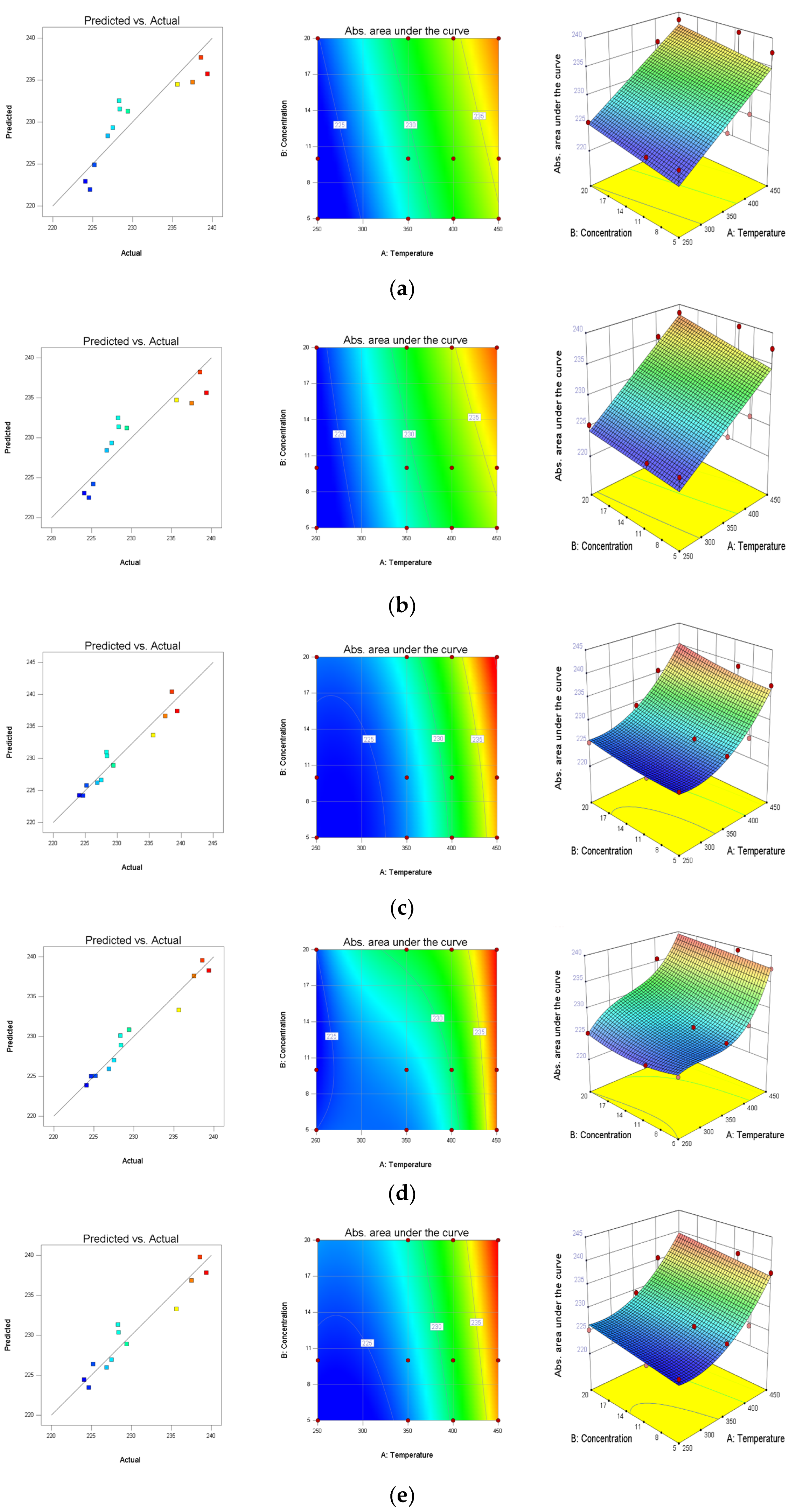
A2	4.19	1	1.20	1.42	6.96	12.19	0.0082

and

Table 12. Analysis of statistical variance.

RMSE	1.84	R-Squared	0.9235
Mean	230.46	Adj R-Squared	0.8948
C.V.%	0.80	Pred R-Squared	0.8478
PRESS	54.02	Adeq Precision	15.352
		BIC	53.793
		AICc	57.56

summarize the statistical parameters for the modified quadratic model, showing that the parameters are properly estimated as the calculated p-values < 0.05. For all response surface design models, high coefficients for determination (R² > 0.90) revealed that variation in responses could not be attributed to random errors but to the effects. On the other hand, for the cubic model, the value of R² _adj (−0.1212) indicates the insignificance of the explanatory variables. Moreover, the difference between R² and R²_adj, which is greater than 0.2, indicates unreasonable agreement as reported in the literature [25,38]. These statistical indicators are supplemented by scatterplots in Figure 2.

The findings summarized in

Table 13. Statistical comparison between the five models.

Model	RMSE	R2	R2adj	R2pred	AICc	BIC	F-Value	Press
Linear	2.76	0.8070	0.7641	0.6808	63.96	62.42	18.81	113.33
2FI	2.90	0.8109	0.7399	0.5631	68.43	64.66	0.16	155.09
Quadratic	2.05	0.9291	0.8700	0.6980	71.4	57.85	5.00	107.20
Cubic	2.19	0.9594	0.8510	-0.1212	144.26	58.68	0.74	398.01
Modified quadratic	1.84	0.9235	0.8948	0.8478	57.57	53.79	32.20	54.02

demonstrate that the modified quadratic model is more precise and can be used to model the used lube oil treated with the red clay process. This accuracy is reflected by the low RMSE error value (1.84) and the high R² and R²_adj ratios (0.9235 and 0.8948, respectively), in addition to the smallest PRESS value (54.02), smallest AICc value (57.57), and the smallest BIC value (53.79), which is compared to the corresponding values obtained by the linear, 2FI, quadratic, and cubic models.

Although the linear model is suggested to model the understudied process, it presents the lowest value of R² and R²_adj ratios (0.8070 and 0.7641, respectively). The cubic and quadratic models, on the other hand, have the highest values of AICc and BIC, whereas the 2FI has the lowest value of R² and R²_adj after the linear model.

In brief, the results indicate the supremacy of the quadratic model of reduced-order over the other models in terms of the minimum RMSE and the highest R² and R²_adj. This finding is in line with that acquired by many scientists confirming that “choosing the best model should concentrate on maximizing the R²_adj and the R²_pred” [34,35,36,37].

Other scientists are advising the use of AICc and BIC for nonlinear models because they perform much better than R² [42].

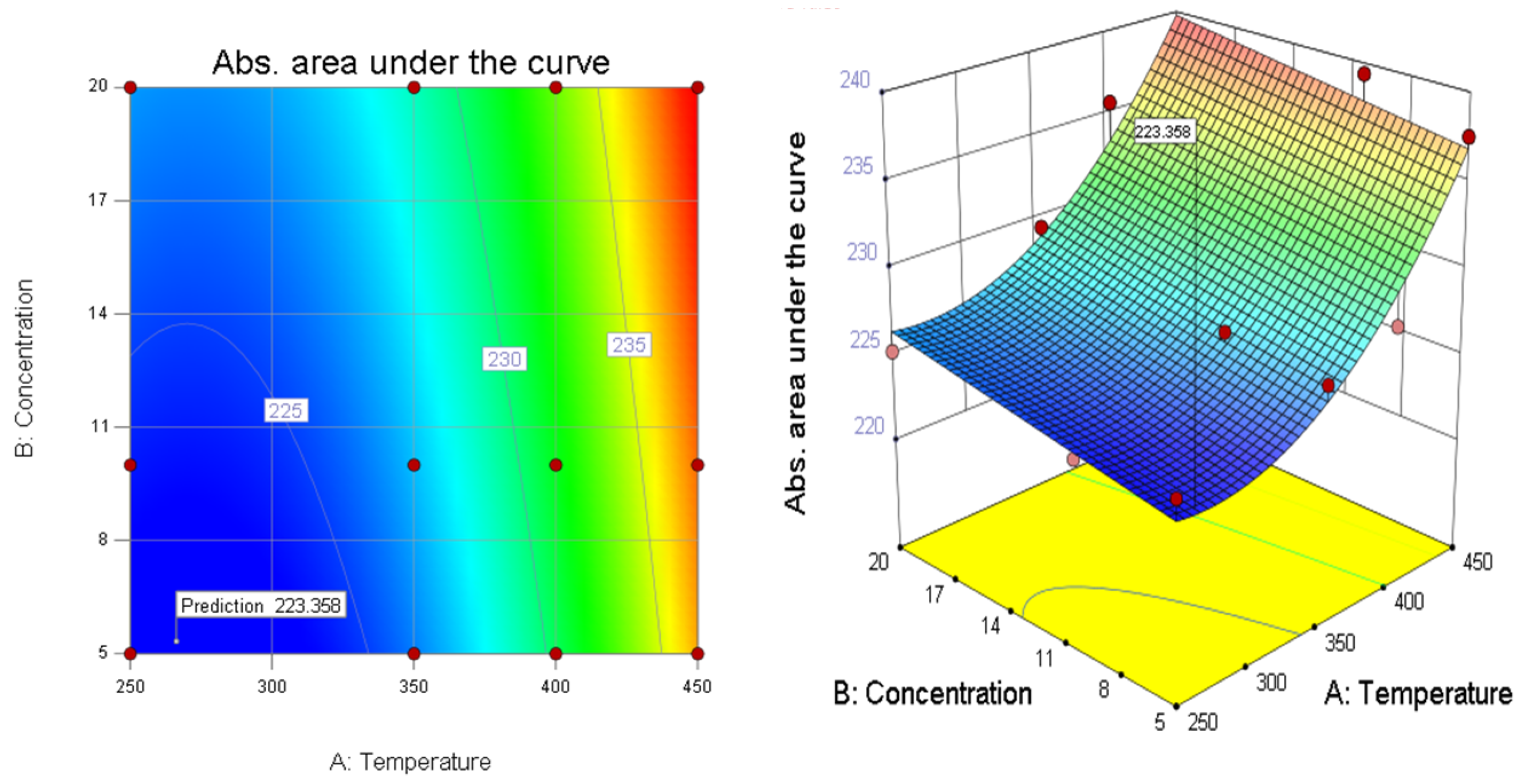
The optimum operating conditions for maximizing production by minimizing the cost of treatment occurs at the minimum absorption under the curve were predicted to be 223.358; this can be achieved at a process temperature of 266.246 °C and 5.331 g clay. These optimum values can be viewed with the contour plot and Three-dimensional 3D curves in Figure 3. Experiments were carried out under these optimal conditions for validating the prediction optimum values. The resulting experimental values of 223.8 is in close agreement with that acquired from the model of regression. Adsorption rates improved with temperature owing to the diffusion of adsorbent molecules into the adsorbent; in addition, solubility and adsorption are inversely linked as temperature impacts the adsorption range [17,43].

This study has revealed that effective oil treatment can be reproduced from natural free-acid clay under optimized process conditions; it is recommended that different types of clays need to be tested, optimized, and mixed to achieve better recycling.

4. Conclusions

This study presents an application of the RSM technique to optimize used the lube oil recycling process treated with natural red clay. Statistical indexes have generated competitive results in comparing the precision and accuracy of the presented models for the used lube oil treatment process. Five different models were tested to find the best fit with the obtained experimental data. The models are linear, 2FI, quadratic, modified quadratic, and cubic models.

Nine statistical indexes (RMSE, BIC, AICc, R², R²_adj, R²_pred, P-value, PRESS, and F-value) were calculated to evaluate model performance.

Obtained results showed that the minimum RMSE value is obtained by the modified quadratic model, whereas the maximum calculated value for R² index is for cubic. However, this model had a low F-value, the highest PRESS, AIC, and BIC making it the least favorable model among the tested ones.

In addition, results show the supremacy of the modified quadratic model in terms of low value of error RMSE (1.84) high values of R² and R²_adj with ratios (0.9235 and 0.8948, respectively), the lowest AICc (57.57), lowest BIC (53.79), comparing to the linear, 2FI, quadratic, and cubic models.

Optimization of the model has provided insightful observation into the process operation conditions for the used lube treatment process, revealing that the optimum operating conditions to maximize production with the minimum cost of treatment happens at minimum absorption under the curve of 223.358; this can be achieved with a temperature of 266.246 °C and a clay amount of 5.331 g. This model can also be used for online state estimation and advanced controlling of the oil recycling process.

References

- Audibert, F. Waste Engine Oils: Rerefining and Energy Recovery; Elsevier: Amsterdam, The Netherlands, 2011. [Google Scholar]
- Cutler, E. Conserve lube oil: Re-refine. [Propane-vacuum-hydrogen process]. Hydrocarb. Process 1976, 55. Available online: https://www.osti.gov/biblio/7361107 (accessed on 19 August 2019).
- Cerny, J.; Strnad, Z.; Sebor, G. Composition and oxidation stability of SAE 15W-40 engine oils. Tribol. Int. 2001, 34, 127–134. [Google Scholar] [CrossRef]
- Ofodu, J.; Anosike, C. Variation in rheological properties of engine oil with usage. Glob. J. Eng. Res. 2003, 2, 95–100. [Google Scholar] [CrossRef]
- El-Fadel, M.; Khoury, R. Strategies for vehicle waste-oil management: A case study. Resour. Conserv. Recycl. 2001, 33, 75–91. [Google Scholar] [CrossRef]
- Brandenberger, S.; Mohr, M.; Grob, K.; Neukom, H.P. Contribution of unburned lubricating oil and diesel fuel to particulate emission from passenger cars. Atmos. Environ. 2005, 39, 6985–6994. [Google Scholar] [CrossRef]
- Pinheiro, C.T.; Pais, R.F.; Quina, M.J.; Gando-Ferreira, L.M. Regeneration of waste lubricant oil with distinct properties by extraction-flocculation using green solvents. J. Clean. Prod. 2018, 200, 578–587. [Google Scholar] [CrossRef]
- Kupareva, A.; Mäki-Arvela, P.; Murzin, D.Y. Technology for rerefining used lube oils applied in Europe: A review. J. Chem. Technol. Biotechnol. 2013, 88, 1780–1793. [Google Scholar] [CrossRef]
- Mohammed, R.R.; Ibrahim, I.A.; Taha, A.H.; McKay, G. Waste lubricating oil treatment by extraction and adsorption. Chem. Eng. J. 2013, 220, 343–351. [Google Scholar] [CrossRef]
- Elbashir, N.; Abdul-Mutalib, M.; Adnan, R. Recycling of used lubrication oil by solvent extraction-a guideline for single solvent design. In Proceedings of the 13th Symposium of Malaysian Chemical Engineers, Hyatt Regency, Malaysia, 13–15 October 1997; pp. 420–427. [Google Scholar]
- Oladimeji, T.E.; Sonibare, J.A.; Omoleye, J.A.; Adegbola, A.A.; Okagbue, H.I. Data on the treatment of used lubricating oil from two different sources using solvent extraction and adsorption. Data Brief 2018, 19, 2240–2252. [Google Scholar] [CrossRef]
- Taha, K.K.; Suleiman, T.M.; Musa, M.A. Performance of Sudanese activated bentonite in bleaching cottonseed oil. J. Bangladesh Chem. Soc. 2011, 24, 191–201. [Google Scholar] [CrossRef]
- Rahman, M.; Siddique, T.; Samdani, S.; Kabir, K. Effect of operating variables on regeneration of base-oil from waste oil by conventional acid-clay method. Chem. Eng. Res. Bull. 2008, 12, 24–27. [Google Scholar] [CrossRef]
- Isah, A.; Abdulkadir, M.; Onifade, K.; Musa, U.; Garba, M.; Bawa, A.; Sani, Y. Regeneration of used engine oil. In Proceedings of the World Congress on Engineering, London, UK, 3–5 July 2013; pp. 54–76. [Google Scholar]
- Hamad, A.; Al-Zubaidy, E.; Fayed, M.E. Used lubricating oil recycling using hydrocarbon solvents. J. Environ. Manag. 2005, 74, 153–159. [Google Scholar] [CrossRef] [PubMed]
- Assunção Filho, J.; Moura, L.; Ramos, A. Liquid-liquid extraction and adsorption on solid surfaces applied to used lubricant oils recovery. Braz. J. Chem. Eng. 2010, 27, 687–697. [Google Scholar] [CrossRef] [Green Version]
- Udonne, J.D. A comparative study of recycling of used lubrication oils using distillation, acid and activated charcoal with clay methods. J. Pet. Gas Eng. 2011, 2, 12–19. [Google Scholar]
- Afolabi, E.A.; Kovo, A.S.; Olalekan, D.A.; Jibrin, A.; Abdulkarrem, A.S.; Suleimam, B. Optimization of the recycle used oil and its fuel quality characterization. Leonardo J. Sci. 2016, 28, 1–14. [Google Scholar]
- Owen, A. Fundamentals of UV-Visible Spectroscopy. Available online: http://agris.fao.org/agris-search/search.do?recordID=US201300126339 (accessed on 19 August 2019).
- Osman, H. Optimizing Model Base Predictive Control for Combustion Boiler Process at High Model Uncertainty. Chem. Biochem. Eng. Q. 2017, 31, 313–324. [Google Scholar] [CrossRef]
- Osman, H. LQ evolution algorithm optimizer for model predictive control at model uncertainty. In Proceedings of the 2014 14th International Conference on Control, Automation and Systems (ICCAS), Gyeonggi-do, Korea, 22–25 October 2014; pp. 1272–1277. [Google Scholar]
- Sacks, J.; Welch, W.J.; Mitchell, T.J.; Wynn, H.P. Design and analysis of computer experiments. Stat. Sci. 1989, 4, 409–423. [Google Scholar] [CrossRef]
- Box, G.; Wilson, K. Royal Statistical Society–Series B. Stat. Methodol. 1951, 13. [Google Scholar] [CrossRef]
- Hardy, R.L. Multiquadric equations of topography and other irregular surfaces. J. Geophys. Res. 1971, 76, 1905–1915. [Google Scholar] [CrossRef]
- Schölkopf, B.; Burges, C.; Vapnik, V. Incorporating invariances in support vector learning machines. In Proceedings of the International Conference on Artificial Neural Networks, Bochum, Germany, 16–19 July 1996; pp. 47–52. [Google Scholar]
- Haykin, S. Neural Networks: A Comprehensive Foundation; Prentice Hall PTR: London, UK, 1994. [Google Scholar]
- Osman, H.; Shigidi, I.; Elkaleefa, A. Optimization of sesame seeds oil extraction operating conditions using the response surface design methodology. Sci. Stud. Res. Chem. Chem. Eng. Biotechnol. Food Ind. 2016, 17, 335–347. [Google Scholar]
- Simpson, T.W.; Mauery, T.M.; Korte, J.J.; Mistree, F. Kriging models for global approximation in simulation-based multidisciplinary design optimization. AIAA J. 2001, 39, 2233–2241. [Google Scholar] [CrossRef]
- Forrester, A.I.; Keane, A.J. Recent advances in surrogate-based optimization. Prog. Aerosp. Sci. 2009, 45, 50–79. [Google Scholar] [CrossRef]
- Amouzgar, K.; Strömberg, N. Radial basis functions as surrogate models with a priori bias in comparison with a posteriori bias. Struct. Multidiscip. Optim. 2017, 55, 1453–1469. [Google Scholar] [CrossRef]
- Osman, H.; Shigidi, I.; Arabi, A. Multiple Modeling Techniques for Assessing Sesame Oil Extraction under Various Operating Conditions and Solvents. Foods 2019, 8, 142. [Google Scholar] [CrossRef]
- Aziz, B.K.; Abdullah, M.A.; Jubrael, K.J. Acid Activation and Bleaching Capacity of Some Clays for Decolourizing Used Oils. Asian J. Chem. 2011, 23, 2449. [Google Scholar]
- D, A. Standard Test Method for ASTM Color of Petroleum Products (ASTM Color Scale). Annual Book of Standards; ASTM International: West Conshohocken, PA, USA, 2007. [Google Scholar]
- Rais-Rohani, M.; Singh, M. Comparison of global and local response surface techniques in reliability-based optimization of composite structures. Struct. Multidiscip. Optim. 2004, 26, 333–345. [Google Scholar] [CrossRef]
- Gary Wang, G.; Dong, Z.; Aitchison, P. Adaptive response surface method-a global optimization scheme for approximation-based design problems. Eng. Optim. 2001, 33, 707–733. [Google Scholar] [CrossRef]
- Yang, B.S.; Yeun, Y.S.; Ruy, W.S. Managing approximation models in multiobjective optimization. Struct. Multidiscip. Optim. 2002, 24, 141. [Google Scholar] [CrossRef]
- Ayati, A.; Moghaddam, A.Z.; Tanhaei, B.; Deymeh, F.; Sillanpaa, M. Response surface methodology approach for optimization of methyl orange adsorptive removal by magnetic chitosan nanocomposite. Maced. J. Chem. Chem. Eng. 2017, 36, 143–151. [Google Scholar]
- Hanrahan, G.; Lu, K. Application of factorial and response surface methodology in modern experimental design and optimization. Crit. Rev. Anal. Chem. 2006, 36, 141–151. [Google Scholar] [CrossRef]
- Bezerra, M.A.; Santelli, R.E.; Oliveira, E.P.; Villar, L.S.; Escaleira, L.A. Response surface methodology (RSM) as a tool for optimization in analytical chemistry. Talanta 2008, 76, 965–977. [Google Scholar] [CrossRef] [PubMed]
- Gendy, T.S.; El-Temtamy, S.A.; El-Salamony, R.A.; Ghoneim, S.A. Comparative assessment of response surface methodology quadratic models and artificial neural network method for dry reforming of natural gas. Energy Sour. Part A Recovery Util. Environ. Eff. 2018, 40, 1573–1582. [Google Scholar] [CrossRef]
- Elkhaleefa, A.; Shigidi, I. Optimization of Sesame Oil Extraction Process Conditions. Adv. Chem. Eng. Sci. 2015, 5, 305. [Google Scholar] [CrossRef]
- Akaike, H. On the likelihood of a time series model. J. R. Stat. Soc. Ser. D Stat. 1978, 27, 217–235. [Google Scholar] [CrossRef]
- Daham, G.R.; AbdulRazak, A.A.; Hamadi, A.S.; Mohammed, A.A. Re-refining of used lubricant oil by solvent extraction using central composite design method. Korean J. Chem. Eng. 2017, 34, 2435–2444. [Google Scholar] [CrossRef]
Figure 1.
The absorbance of treated oil.
Figure 2.
Comparison between the models: predicted vs. actual, contour and 3D curves. (a) Linear model, (b) 2FI model, (c) quadratic model, (d) cubic model, and (e) modified quadratic model.
Figure 3.
Contour and 3D curves for optimum design values for the modified quadratic model.