All articles published by MDPI are made immediately available worldwide under an open access license. No special
permission is required to reuse all or part of the article published by MDPI, including figures and tables. For
articles published under an open access Creative Common CC BY license, any part of the article may be reused without
permission provided that the original article is clearly cited. For more information, please refer to
https://0-www-mdpi-com.brum.beds.ac.uk/openaccess.
Feature papers represent the most advanced research with significant potential for high impact in the field. A Feature
Paper should be a substantial original Article that involves several techniques or approaches, provides an outlook for
future research directions and describes possible research applications.
Feature papers are submitted upon individual invitation or recommendation by the scientific editors and must receive
positive feedback from the reviewers.
Editor’s Choice articles are based on recommendations by the scientific editors of MDPI journals from around the world.
Editors select a small number of articles recently published in the journal that they believe will be particularly
interesting to readers, or important in the respective research area. The aim is to provide a snapshot of some of the
most exciting work published in the various research areas of the journal.
With renewable generation resources and multiple load demands increasing, the combined cooling, heating, and power (CCHP) microgrid energy management system has attracted much attention due to its high efficiency and low emissions. In order to realize the integration of substation resources and solve the problems of inaccurate, random, volatile and intermittent load forecasting, we propose a three-stage coordinated optimization scheduling strategy for a CCHP microgrid. The strategy contains three stages: a day-ahead economic scheduling stage, an intraday rolling optimization stage, and a real-time adjustment stage. Forecasting data with different accuracy at different time scales were used to carry out multilevel coordination and gradually improve the scheduling plan. A case study was used to verify that the proposed scheduling strategy can mitigate and eliminate the load forecasting error of renewable energy (for power balance and scheduling economy).
As opposed to traditional power system problems, the CCHP (combined cooling, heating, and power) microgrid’s energy optimization management problem is more difficult to solve. New energy generation accounts for a large proportion of the energy system. New energy generation, such as wind power generation and photovoltaic power generation, is vulnerable to the external environment. Compared to other forms of traditional power generation, these new energy generation forms usually have random, fluctuating, and intermittent characteristics. Therefore, high-precision wind and light resources and load prediction algorithms are needed to support the energy management of a CCHP microgrid. However, the accuracy of these new energy power predictions is difficult to guarantee. The longer the time span is, the lower the prediction accuracy. For example, when a current wind power forecast is made, the error can reach 25%~40%, and the intraday prediction error may be larger. With the continuous development of big data short-term and ultrashort-term forecasting technologies, historical data such as renewable energy output and heat and cold loads have accumulated significantly. Prediction accuracy and speed have also improved significantly, but it is still difficult to guarantee the efficient and economic operation of a CCHP microgrid.
In addition, current research on the energy management of a CCHP microgrid has mainly concentrated on a single time scale, mostly for economic operation. However, during actual system operation, the output fluctuations of wind power and photovoltaic power are very large. In addition, the optimization results formulated on a long-term scale are not actually optimal solutions, or even feasible solutions [1,2,3]. These directly affect the economics and safety of a system’s optimized operation.
Therefore, many scholars are paying more and more attention to the impact of power fluctuations on the optimal operation of a system. Zhou established a dynamic scheduling model for a CCHP microgrid that takes into account additional opportunity benefits. Using a time-sharing electricity grid and grid-connected operating conditions, a simulated annealing particle swarm optimization algorithm was used to solve the problem [4,5]. In order to cope with the uncertainty of the thermal power load and the output of renewable energy such as wind and light, Sang and Zhang established a stochastic optimization operation model of a CCHP microgrid [6,7]. Aiming at the stochastic characteristics of cold and heat loads and renewable energy output, Grover-Silva and Ji established a pre-economic scheduling model for a cold-heat-powered microgrid based on interval planning [8,9]. Moradi proposed an energy management method for a cogeneration system based on a fuzzy programming optimization algorithm [10]. Smith proposed a method based on quantitative analysis to deal with the uncertainty of a cogeneration system under different operating strategies [11].
The above-mentioned literature mainly focused on the planning of a cold-heat-electric cogeneration microgrid and research on economic dispatches. However, recent research has not fully reflected the prediction error of renewable energy output and loads. The influence of unplanned instantaneous fluctuation power on the energy management of a cogeneration microgrid has also not been considered, so dispatches do not match the actual operation of the system perfectly. In order to cope with the large-scale wind power access and energy optimization management problems of a traditional microgrid with multiple time scales and to learn from the multi-time-scale-coordinated active power allocation scheme adopted by large power grids, many scholars have carried out a large number of multi-time-scale energy management optimization studies on hybrid microgrids [12,13,14,15,16,17]. Gu has proposed an intraday model predictive control method to reduce the impact of prediction errors on the CCHP microgrid [1]. Luo proposed a two-stage energy management method that considers the characteristics of a house during the day and minimizes the impact of a system on the upper-level power grid, continuously revising the plan [2]. Tian proposed a multi-time-scale energy coordination optimization method for a hybrid microgrid and a cogeneration hybrid microgrid, which formulates the unit combination plan on an hourly time scale. Power fluctuations are suppressed by the microcombustion engine and the energy storage system on the “minute” and “second” time scales, respectively [3]. However, this strategy ignores the coordination between long-term and short-term scheduling and does not consider the overall economics of the system. Although these scheduling strategies can largely eliminate the volatility of intermittent energy and loads, there are various problems with these strategies:
Insufficient consideration of the treatment of uncertainty in the economic scheduling;
Long-term and short-term coordination, coordination between schedules, and the overall economics of the system are not considered comprehensively; and
The feedback correction for the optimization control process is not considered in the optimization scheduling process. When the fluctuations in the load and renewable energy output are large but on a short time scale, the scheduling strategy may lose its effect.
In this paper, these factors are fully considered. A three-stage coordinated optimization scheduling strategy is proposed for a CCHP microgrid in grid-connected operation mode, which uses different precision prediction data on different time scales. It gradually refines and improves the dispatch plan to reduce and eliminate the impact of renewable energy output and load forecasting error on the power balance and operational economy of the dispatch plan. Finally, an example is given to verify the rationality and effectiveness of the proposed energy management strategy for a CCHP microgrid (based on three-stage coordinated optimization).
2. CCHP Microgrid Description and Modeling
The CCHP microgrid involves many devices, including microgas turbines, absorption refrigerators, electric refrigerators, waste heat recovery devices, heat exchangers, and distributed renewable energy [18,19]. Figure 1 shows the system structural diagram of a CCHP microgrid.
During the modeling process, there are several parts to take note of:
(I) A microgas turbine: The optimization results are based on two economic scheduling models. When the operating conditions of the microgas turbine under the two models are the same in certain periods, the operating conditions of the microgas turbine will not change with future scheduling strategies. When the operating conditions of the microgas turbine under the two models are inconsistent in certain periods, the operating conditions of the microgas turbine can change within the threshold boundaries of these periods with future scheduling strategies;
(II) Battery: In accordance with the optimization results obtained by the two economic dispatching models, operating conditions with three consistent scheduling curves in the charging and discharging states of the battery are preferentially selected. Secondly, operating conditions in which two scheduling curves are consistent in the states of charge and discharge of the battery during certain periods are selected. Finally, economic-scheduling-optimized charging and discharging conditions are selected;
(III) Other equipment: As opposed to economic scheduling optimization, mixed-integer linear programming (MILP) optimization obtains a set of interval scheduling instructions, which cannot give optimal scheduling instructions. Therefore, the economic dispatch plans of other equipment directly select the scheduling results of the recent economic scheduling optimization.
Finally, for the operation strategy adopted by the microgas turbine, three sets of daily plans are obtained: (1) The operating period during which the microgas turbine does not change. Here, PDh = [, , , , , , , , , ], where is the charge power of the microgas turbine in interval Dh, is the electricity demand of the electric chiller in interval Dh, and and represent the charge/discharge power of the battery (BT) in interval Dh, respectively. and represent the power supplied by the main grid that is sold to the main grid in interval Dh. represents the power output of the gas boiler in interval Dh. is the heat required by the absorption chiller to meet the cooling demands in interval Dh. and represent the thermal power stored/released by the thermal storage tank (TST) in interval Dh. (2) The second plan is the operating period in which the microgas turbine is allowed to be adjustable within the control range: PDh = {[, ], [, , , , , , , , ]}, and (3) The third plan is the charge and discharge status of the battery during the entirety of the day’s operation period (UDh = [, ], where and represent the charge/discharge state of the BT in interval Dh, respectively).
3. Three-Stage Optimization Framework
Since the prediction accuracy has an inverse relationship with the time span, and considering the load fluctuation characteristics and the control characteristics of the distributed units in the system, this paper proposes a three-stage optimization framework for the CCHP microgrid. The framework includes a day-ahead economic scheduling stage, an intraday rolling optimization stage, and a real-time adjustment stage. Figure 2 shows the relationship between these three stages. For a comprehensive consideration of the impact of the computing speed and computing effects, the economic scheduling strategy is set at 24:00 every day, while the intraday rolling optimization is made every 15 min and the real-time adjustment is developed every 5 min [1]. As time goes by, the time period corresponding to the intraday and real-time adjustment plans continues to move forward. In this paper, the scheduling range (length of the period) of the economic scheduling, intraday rolling optimization, and real-time adjustment was set to 24 h, M hours (the scrolling time needed to be optimized), and 5 min, respectively.
(a) Day-ahead economic scheduling stage: During the day-ahead economic scheduling stage, both the economics and safety of the system are considered. The start-stop plan, output value, and interaction power in terms of the grid of the core joint equipment over 24 h are given by the MILP-based economic scheduling joint decision system. The scheduling values mentioned in the last chapter are directly substituted into the predictive control optimization scheduling stage of the economic scheduling model as an input, and other unknowns in the model are solved. The dispatcher adjusts the conservative parameters according to the historical data of the long-term observations and selects a reasonable economic dispatch plan, thus reducing the impact of uncertainty on the energy management of the CCHP microgrid.
(b) Intraday rolling optimization stage: During the actual operation of a CCHP microgrid, considering the randomness of renewable energy and load power, power data are often difficult to predict accurately. Therefore, it is necessary to add a better real-time intraday predictive control optimization scheduling link to correct the economic dispatch plan. The intraday predictive control optimization scheduling stage is executed every 15 min, and the cold–heating load and wind–light forecast data are continuously updated in real time to realize the correction of the economic dispatch plan. The CCHP microgrid energy management system’s cold and hot load and wind power generation power prediction module continuously predicts the cold and heat load, wind power, and photovoltaic power according to real-time operational data. It also continuously optimizes the CCHP microgrid for future periods. The operating conditions provide a power reference point for the real-time adjustment stage.
(c) Real-time adjustment stage: The main purpose of real-time adjustment is to mitigate or eliminate random fluctuations in load and renewable resource output. At this stage, on the basis of the difference between the short-term forecast results and the real-time data, the complementary characteristics of multiple energy sources and the coordination equipment are used to coordinate the fluctuations of the load and the renewable energy output.
3.1. Day-Ahead Economic Scheduling Stage
During the day-ahead economic scheduling stage, in order to determine the optimal scheduling order, predictions and optimizations are performed at each time interval. An economic dispatch model based on a model predictive control (MPC) method is used, taking into account the operating status and the operating-rated power limit of all equipment in the system. By combining the prediction results from the intraday rolling optimization stage, the real-time adjustment stage, and the future time range (from k to the Mth time interval thereafter), the day-ahead economic scheduling stage model can be solved. By solving the model, we can get the best scheduling scheme in this stage.
3.1.1. Objective Function
In order to determine the initial operation of the system scheduling, we take into account the income and cost amounts of different parts. With the goal of maximizing economic benefits, the objective function of the economic dispatches is formulated as shown below:
where is the cost of interacting with the main grid, is the cost of the natural gas, is the cost of the aging battery, is the cost of operating and maintaining the system, is the tariff for purchasing power from the main grid (¥/kWh), is the tariff for selling power from the main grid (¥/kWh), is the cycle cost of the battery (¥/per time), is the tariff for natural gas (¥/per time), is the cost of operating and maintaining different units, is the calorific value of natural gas (kW), is the power of the gas boiler in period t (kW), is the thermal load power in period t (kW), is the heat required by the absorption chiller to meet the cooling demand in period t (kW), and , is the thermal power stored/released by the thermal storage tank (TST) in period t (kW).
3.1.2. System Restrictions
In each device, restrictions such as cooling balances, heating balances, electricity balances, and operational restrictions must be considered in the system to keep the balance of the system. The system operation constraints are shown as follows:
the cold balance constraint is
the thermal balance constraints are
and the electrical balance constraints are
After solving the equation above, the optimal schedule in this period can be obtained. In the next period, only the solution results obtained in the previous time period are used to ensure the real-time nature of the data. In addition, the time scale will continue to move forward in the next period. The initial operation of the system scheduling is solved in this stage.
3.2. Intraday Rolling Optimization Stage
In order to reduce or eliminate the random fluctuation of the load and renewable resource output and reduce the deviation between the economic dispatch plan and ultrashort-term scheduling, we added a rolling optimization link. Its purpose is to use the latest information (such as the renewable energy and real-time power data of cold and heat loads or the latest weather information) from the prediction model calculation to correct the subsequent renewable energy and load power values, and thus the dispatching plan for the subsequent time period is obtained. Rolling optimization is a process that constantly corrects and constantly refreshes the economic dispatch plan.
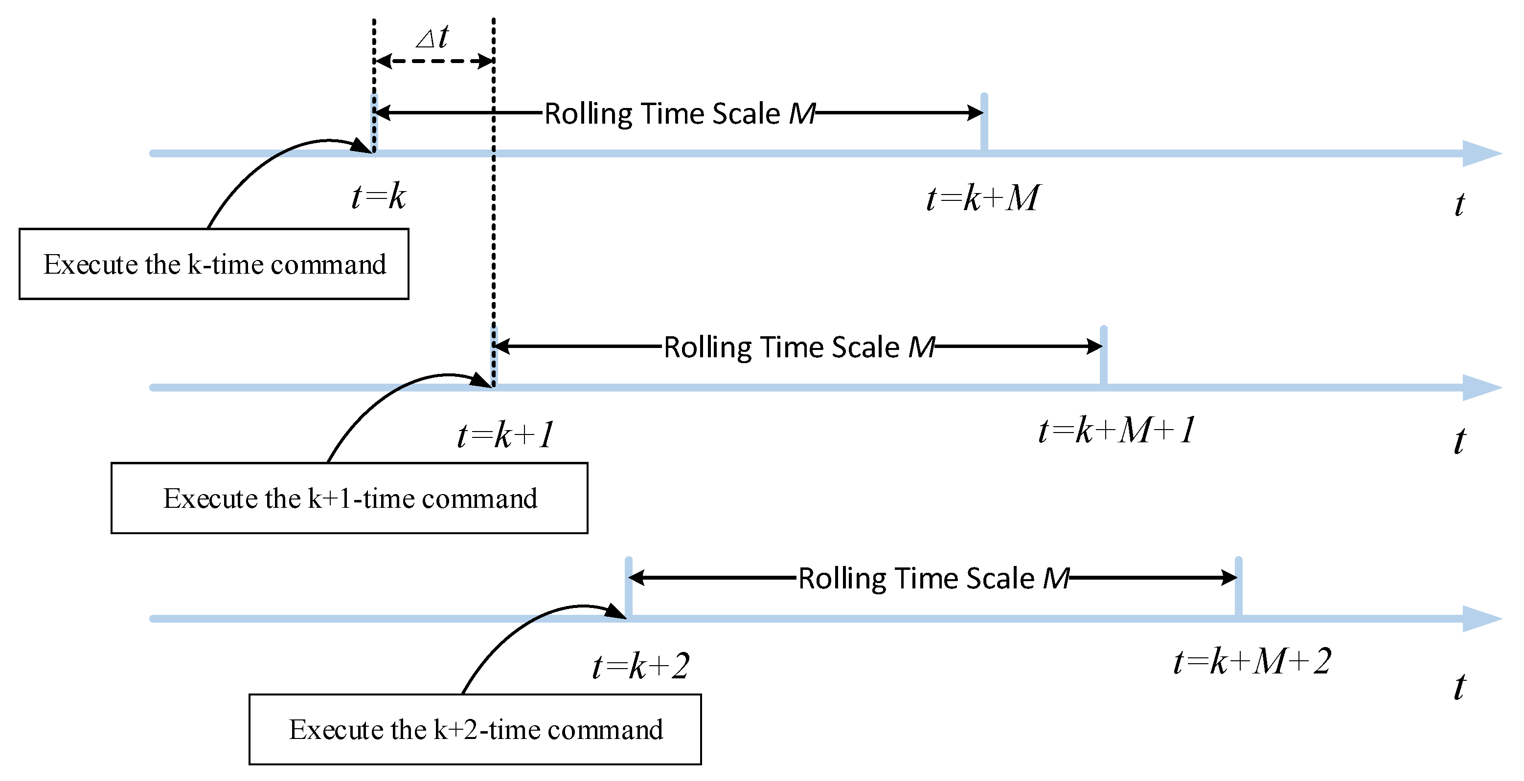
The rolling optimization stage mainly consists of three parts: prediction modeling, feedback correction, and rolling optimization. The basic idea is to obtain the renewable energy output value and load data of the system in the predicted time domain based on the prediction model and the measured output. At each sampling time k, the system’s renewable energy output and load are predicted, and the scheduling algorithm sequence in the future control time domain is calculated using the optimization algorithm (but only the first scheduling instruction of the k-time optimization results is sent to the system). At sampling time k + 1, the entire above optimization step is repeated with the new output measurements (the meaning of scrolling optimization), as shown in Figure 3. It can be seen that the rolling optimization optimizes the target in a limited time domain, and the optimized performance index only involves limited time in the predicted time domain (from the current time). In the next period, this optimization period moves forward. During this rolling optimization process, the prediction information is continuously updated, and at the same time, through feedback correction, historical information is also adopted. This scheme can effectively overcome the effects of errors in the system due to prediction model errors and some uncertainties.
Therefore, on the basis of existing research theories, this paper proposes an intraday rolling optimization strategy based on model predictive control. We focus on the optimal performance of a closed-loop control in an optimization period in the future. Feedback correction is introduced to effectively correct the deviation of the optimal scheduling result caused by the prediction error and random factors, which improves the precision of the optimization control and provides an adjustment reference power point for the real-time adjustment phase.
3.2.1. Prediction Model
According to the length of the forecast period, renewable energy and cold and heat power forecasts are generally classified into long-term, medium-term, short-term, and ultrashort-term forecasts. An ultrashort-term power forecast mainly predicts the future renewable energy and load power data of the system (5~60 min). In this section, the time interval of the economic dispatch phase, which is based on model predictive control, is 15 min. Therefore, the predictive module of renewable energy and cold and hot power is an ultrashort-term forecast.
At present, there are many methods for predicting ultrashort-term renewable energy and load, mostly using Kalman filtering [21,22,23], artificial neural networks [24], time series [25], and the gray theory method [26,27]. Compared to other prediction methods, the gray prediction method does not need to determine whether the renewable energy and the thermal power fluctuations follow a normal distribution and does not require large sample statistics. There is also no need to change the prediction model at any time based on changes in renewable energy and hot and cold power [28]. Its predictive model is easy to operate and has short-term precision, which is more suitable for online ultrashort-term forecasting.
The specific steps of the grey model (1,1) (GM (l, 1)) prediction model are shown here:
Step 1. Input the raw renewable energy and hot and cold power sequence :
where n is the time series of observational data, and represents wind power, photovoltaic power, or thermal power load.
Step 2. Accumulate the renewable energy and cold and hot power sequences to get a new accumulation sequence:
where
Step 3: Establish the general differential equation for the gray dynamic model (first-order models with one variable) to clarify . The sequence mentioned in step 1 is selected as the initial value here for calculation:
where ci represents the development coefficient, and di is the gray amount.
Using the least squares method, we can get the following program:
where
Step 4. Obtain an approximate solution for the differential equation and calculate the renewable energy and the hot and cold power according to the corresponding formula.
The approximate solution to the differential equations is
The equation for renewable energy and hot and cold electricity power is
where is the ultrashort-term renewable energy and cold and hot power forecasting.
Step 5. Take k = 1, 2, …, n for the distribution of the above formula to obtain the fitting sequence of the original sequence (j), where j = 1, 2, …, n.
Step 6. Take k = 1 + n, k = 2 + n, …, k = m + n for the distribution of the above formula to obtain the sequence of predicted values after the original sequence (j), where j = 1, 2, …, m.
3.2.2. Feedback Correction
Due to the nonlinear factors, time variation factors, and other influencing factors of the actual control target, the scheduling instruction data of predictive control based on the open-loop model is difficult to be consistent with the actual running instruction data. Therefore, after the scheduling instruction is executed, the scheduling instruction at the next moment will have a certain deviation from its power prediction value, that is, the amount of power imbalance. Since the prediction error is unavoidable, it is necessary to introduce the prediction error feedback link and correct the output based on open-loop model predictive control through the actual measured information, and then perform a new round of optimization. This enables the scrolling optimization to be based not only on the model, but also on the feedback information (to form a closed-loop optimization).
The fitted sequence of the original sequence is obtained through step 5 of the above prediction module. First, it is compared to the original load series, and the root mean square relative error indicator is used to evaluate the prediction results:
If the fitting accuracy is high enough, step 6 of the above prediction module can be used to obtain the predicted value sequence . If the fitting accuracy is poor, a residual sequence needs to be constructed:
While I ≥ k0, I = k0, k0 + 1, …, n, the residual sequence has a consistent symbol. For the residual sequence |(k0)|, |(k0 + 1) |, …, |(n)|, the predicted value |(k0)|, |(k0 + 1) |, …, |(n)| can be obtained by using the above GM (1,1) model.
The next predicted sequence of the prediction model is corrected by using the weighted value of the prediction error vector (described above). The corrected prediction vector of can be obtained:
where the value of “±” is consistent with the sign of the residual sequence .
3.2.3. Rolling Optimization
Model predictive control uses a rolling finite time domain optimization strategy, namely rolling optimization. The main goal of rolling optimization is to use the latest information (through prediction model calculation, feedback correction of the resulting renewable energy, and the thermal power load) to obtain optimal scheduling instructions for the subsequent period. Rolling optimization is performed by continuously correcting the economic scheduling plan and using its scheduling instructions as the adjustment basis for the real-time adjustment layer. The following—Δ, Δ, Δ, Δ, Δ, Δ, Δ, Δ, Δ, Δ—are the adjusted power of the microgas turbine, the electric refrigeration machine, the battery charge and discharge, the interaction power with the grid, the gas boiler, the absorption chiller and heater, and the heat release of the heat storage tank in the day-ahead economic scheduling stage, where the unit of measure for power is kW.
The goal of the optimized operation of the CCHP microgrid is to minimize the operating costs of the system. Therefore, its objective function is
where M is the control time domain of the scheduling period. is the system operating cost, including the cost of the CCHP microgrid and power grid interaction. is the cost of purchasing natural gas, and is the penalty cost for the change in the charge and discharge power of storage. Here, the unit of measurement of the cost is yuan.
The cost of the CCHP microgrid and power grid interaction is
where is the electricity price of purchasing electricity from the grid for the system during the period . is the power that the system purchases from the grid during the period t. is the price at which the system sells electricity to the grid during the period t. is the power that the system sells to the grid during the period t, and μgrid is a penalty function for the power change that interacts with the grid. M represents the time interval. For these variables, the unit of measurement of the electricity price is yuan/kWh, and the unit of measurement of power is kW.
The cost of purchasing natural gas is
where is the system purchase price of natural gas during the period t. is the fuel power consumed by the microgas turbine in the period t. is the fuel power consumed by the gas boiler in the period t. Hng is the calorific value of natural gas. Here, μmt and μb are the penalty functions for the power variations of the microgas turbine and the gas boiler, respectively.
The penalty cost for the change in the charge and discharge power of the storage is
where μbt is a penalty function for the change in the battery charge and discharge power.
3.2.4. System Restrictions
The system constraints mainly include the electric power balance, thermal power balance, cold power balance, operational constraints of each device in the microgrid, and constraints on interactions with the grid.
The cold balance constraint is
where COPac, COPec are the refrigeration coefficients of absorption chillers and electric chillers, respectively. is the cooling load (kW) of the period t.
The thermal balance constraints are
where is the heat power (kW) recovered by the waste heat recovery device in the period t.
The electrical balance constraints are
the gas boiler constraints are
the microgas turbine constraints are
and the heat storage tank (TST) constraints are
In terms of the battery (BT) constraints, in order to prevent the battery from charging and discharging frequently, this section sets an operation mode for it. When the battery charge and discharge plan value is not zero, the battery charge and discharge state is the M plan value of the current time. When the battery charge and discharge plan value is zero, the battery charge and discharge plan value is traced back to the plan in which the battery charge and discharge plan value is not zero:
The interaction power constraints in terms of large grids are
Through the optimized scheduling phase based on model predictive control, the scheduling plan value with a time scale of 15 mins is obtained: PIh = [, , , , , , , , , ].
3.3. The Real-time Adjustment Stage
The stochastic fluctuations of the cold and hot power load and renewable energy, the prediction error, and the advanced predictive control process cannot perfectly match the system scheduling plan with the actual load demand. In order to balance the intermittent energy output and load fluctuations, it is necessary to introduce a real-time adjustment stage at a time after the predictive control process. According to the real-time error situation of wind power output and cold and hot power load demand, the real-time adjustment stage further optimizes the output of the joint supply equipment to ensure the accuracy and anti-interference of the dispatching instructions.
3.3.1. Objective Function
In order to reflect scheduling instructions based on the model predictive control optimization scheduling stage, the real-time adjustment stage complies with the output plan value of each joint unit in the upper-level scheduling plan and only adjusts the output of each unit at the current time scale. The goal of this stage is to reduce the number of equipment adjustments and improve system security and stability. The objective function is shown below:
where is the total adjustment of the system. Here, Δ, Δ, Δ, Δ, Δ, Δ, Δ, Δ, Δ, Δ are the adjustment powers (kW) of the microgas turbine, electric refrigerator machine, battery charge and discharge, gas boiler, absorption chiller, and heat storage tank in the real-time adjustment stage, respectively. In addition, w1, w2, w3 are the cold and thermoelectric adjustment weight coefficients, and the distribution of the weight coefficients is assigned according to the worst degree of influence of the cold and thermoelectric uncertainty on the system, satisfying w1 + w2 + w3 = 1.
3.3.2. System Restrictions
The system operation constraints are shown as follows.
The cold balance constraint is
the thermal balance constraints are
the electrical balance constraints are
the gas boiler constraints are
the microgas turbine constraints are
the heat storage tank (TST) constraints are
the battery (BT) constraints are
and the interaction power constraints in terms of large grids are
3.4. The Proposed Three-Stage Optimization Energy Management Structure
The coordinated optimization scheduling strategy proposed in this paper includes three stages. Figure 4 shows the implementation process of the overall three-stage optimization energy management structure. It includes an economic optimal scheduling control problem for calculating errors and an intraday rolling optimization control problem to reduce or eliminate the random fluctuation of load and renewable resource output and reduce the deviation between the economic dispatch plan and ultrashort-term scheduling. Finally, it includes a real-time adjustment scheduling model to balance the intermittent energy output and load fluctuations. The three-stage coordinated optimization scheduling strategy procedure is as follows (shown in Figure 4):
Step1. At each time scale, the updated historical data can be obtained and used to predict the power load for the next time horizon. The state of the battery and the thermal storage tank can be updated from Step 6;
Step 2. Then, the MILP problem based on the predicted information from step 1 is solved. P* and U* can be calculated for the next time horizon;
Step 3. Then, the GM (1,1) model is used to evaluate the predicted results. The prediction error feedback correction of the resulting renewable energy and the thermal power can be obtained. Further, a prediction error feedback link can be built;
Step 4. The MILP problem is solved based on the prediction information from step 3. The new P* and U* (with a feedback link) can be calculated for the next time horizon;
Step 5. The prediction power load obtained from the above steps is monitored, and the real-time data are considered to adjust the schedule and apply the units of power P to the CCHP microgrid;
Step 6. The time scale is updated. If the time scale reaches the next time horizon, t = t + Δt, the updated data are fed back, and we jump to step 2. Otherwise, t = t + Δt’, and we jump to step 5.
4. Case Study
This chapter uses an office building in Shanghai as a reference object. The building has 20 floors, with each floor having an average height of 3.8 m, and the building’s area is 8000 m2. The entire building is equipped with photovoltaic power (1 × 50 kW), a gas turbine (1 × 200 kW), a gas boiler (1 × 500 kW), an electric refrigerator (1 × 100 kW), an absorption refrigerator (1 × 200 kW), a battery (1 × 500 kWh), a heat storage tank (1 × 500 kWh), a thermal interactor (1 × 200 kW), and a wind turbine (1 × 50 kW). Figure 5 shows the cooling and heating power load and photovoltaic output on a typical summer day. The electricity price data shown in Table 1 are the purchase/sale price of electricity for the system and the main grid. Table 2 shows the capacity and corresponding efficiency parameters of various types of equipment for combined heating and cooling microgrids. Natural gas is used as the fuel for the microgas turbines and gas boilers. The unit price is 3.24 yuan/m3, and the unit heat value of natural gas is 9.78 kWh/m3.
In order to verify the rationality and effectiveness of the algorithm, this section analyzes it from the following three perspectives: (1) the selection of the rolling duration of intraday rolling optimization; (2) an analysis of the simulation results of optimal scheduling; (3) and a comparison of the optimization results and the algorithm performance of different scheduling strategies at other multi-time-scales. This paper assumes that the number of day-ahead scheduling periods is 24, that the duration is 1 h, and that the time interval for the intraday predictive control scheduling phase is 15 min. The length of the control time domain is M h (where the prediction duration and the control duration are equal and need to be optimized). Five minutes is selected as the time scale of the real-time adjustment phase, so three real-time adjustments must be performed within the time interval of the intraday predictive control scheduling phase. The simulation time selects three different seasonal typical days (summer, winter, and the transition season), and the analysis of the case focuses on summer data.
The predicted time domain length or the rolling optimized duration indicates how many steps are needed to predict the output value from the current moment, and the control time domain length is the number of control variables to be determined during the optimization objective. The selection of the prediction time domain length will affect the robust stability and rapid operation of the system. The selection of the control time domain length for specific control objects can be adjusted and selected according to the system’s requirements for the optimization target. The basic requirement for controlling time domain selection is less than or equal to the predicted time domain length. In order to facilitate the analysis, we chose the same control time domain and predicted time domain, that is, the rolling optimization time is M h, and the time interval is 15 min. Considering comprehensive economics and computing time, we selected the rolling time M to be 4 h for this paper’s intraday predictive control optimization scheduling stage (that is, 16 sampling points) [1].
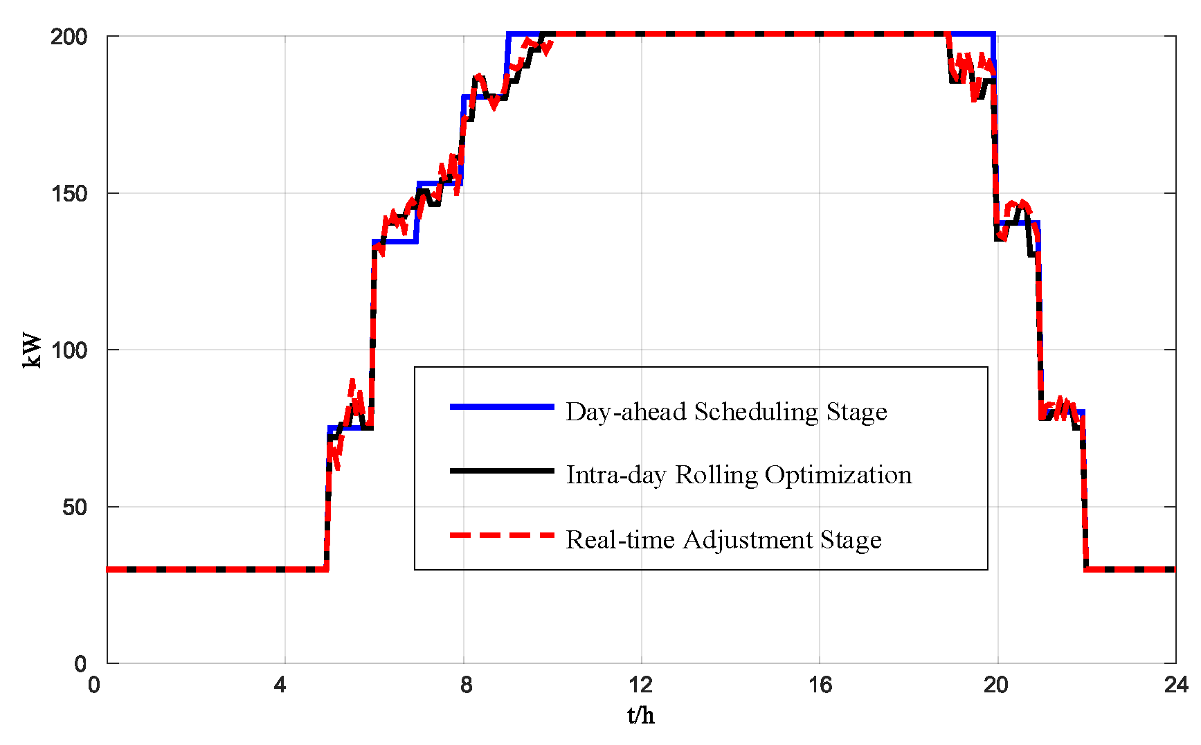
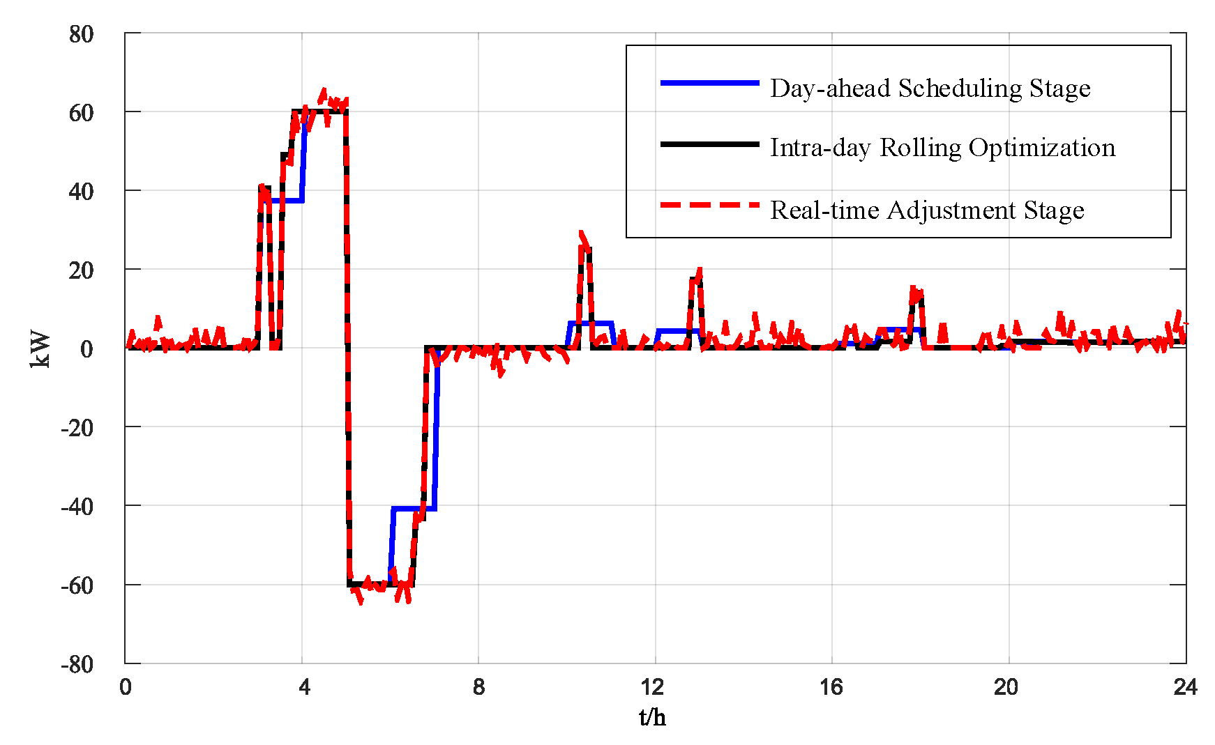
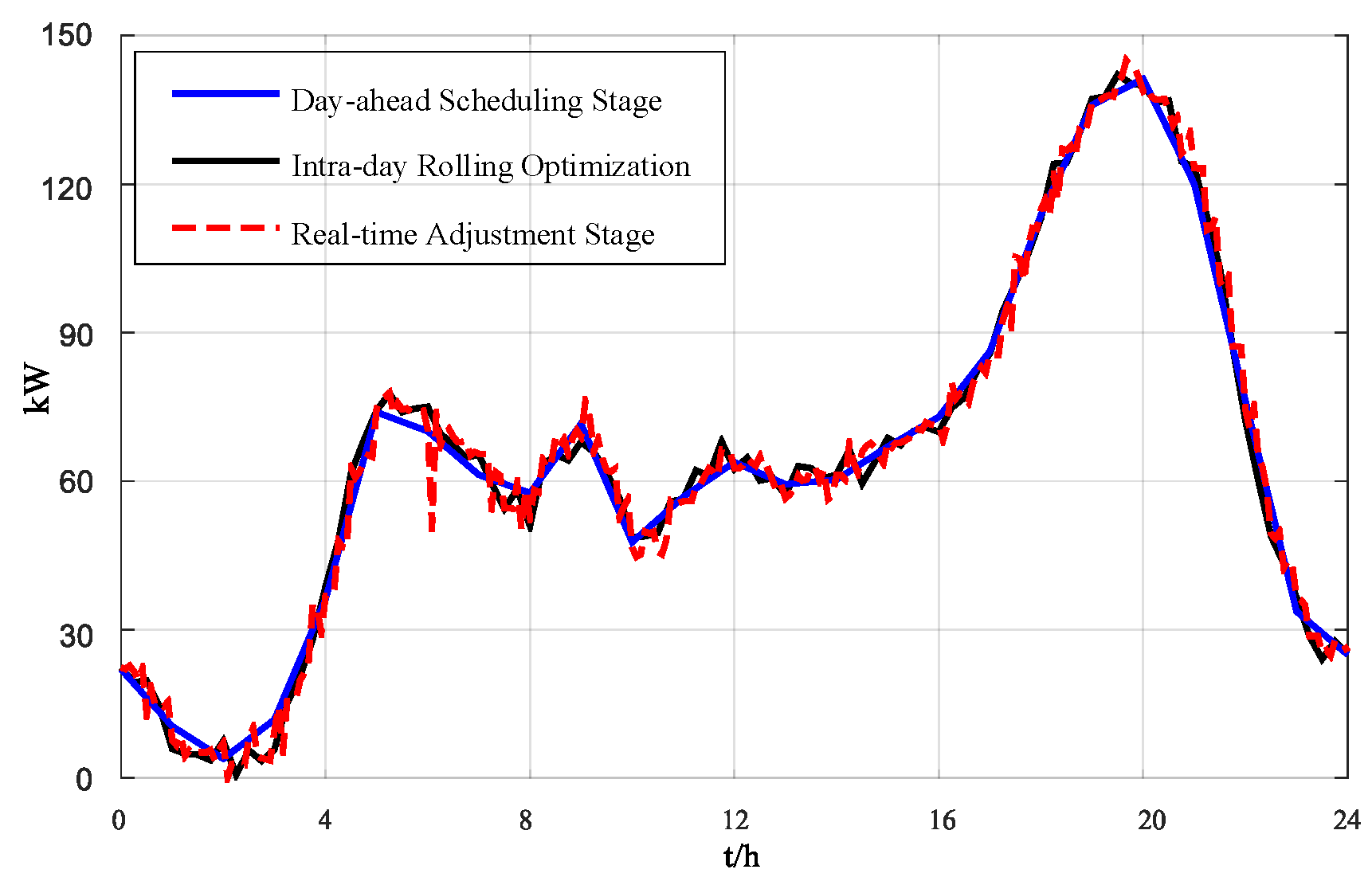
The results of the optimized operation of each device in the system at multiple time scales are shown in Figure 6, Figure 7, Figure 8, Figure 9, Figure 10 and Figure 11. Figure 6 shows the optimization results of the microgas turbine at multiple time scales. Figure 7 shows the results of the battery charge and discharge power optimization at multiple time scales. Figure 8 shows the optimization results of power interactions with the power grid at multiple time scales. Figure 9 shows the results of optimizing the cooling power of an electric refrigerator at multiple time scales. Figure 10 shows the results of optimizing the refrigeration power of an adsorption refrigerator at multiple time scales. Figure 11 shows the results of optimizing the heat absorption power of the heat exchanger at multiple time scales. In these figures, the blue line is the day-ahead scheduling plan, the black line is the intraday rolling optimized scheduling, and the red dotted line is the scheduling instruction for real-time adjustment.
As can be seen from Figure 6, Figure 7, Figure 8, Figure 9, Figure 10 and Figure 11, when the power purchase price is relatively low, the main grid provides the main electrical load of the system. When the power purchase price is relatively high, the microgas turbine provides the main system power load, charging excess batteries or selling them to the grid. The battery discharges outward when the electricity price is high, and charges when the electricity price is low. The battery is charged and discharged once per day, which is conducive to reducing the operating cost of the system and extending the service life. When the purchased electricity price is relatively low, the electric refrigerator consumes more power to provide the cooling load. When the purchased electricity price is relatively high, the cooling capacity of the electric refrigerator is relatively reduced. This is because a large amount of waste heat is generated by the gas turbine that provides more electrical energy, and the absorption refrigerator absorbs the waste heat for cooling. The heat exchanger meets the heat load demand of the system by absorbing the waste heat.
At the same time, it can be seen that day-ahead planning and intraday rolling optimization are based on hours, and the scheduling plan is rough. However, the intraday rolling optimization is revised (compared to day-ahead planning). In order to balance the power and load fluctuations of intermittent energy sources, all cogeneration equipment and energy storage systems share the power fluctuations to reduce the impact of the system on the operation of the large power grid. During the real-time adjustment phase, the core cogeneration equipment’s operating power closely tracks the planned value of the day’s predictive control optimization phase and compensates for the power imbalance caused by the cooling, heating, and electricity loads and renewable energy sources (within the limits of the technology).
4.2. Algorithm Performance Analysis
In order to illustrate the effectiveness of the proposed multi-time-scale coordinated optimization algorithm and its practicality in the actual environment, this chapter will discuss and compare the following aspects: (1) the operating cost of the system using different multi-time-scale optimization strategies; (2) the calculation time; and (3) the operational cost and ideal cost of the proposed method (summer, winter, and the transitional season).
In the actual operation of CCHP microgrids, there are generally two typical operation modes: following the thermal load (FTL) and following the electric load (FEL). In order to prove that the algorithm proposed in this paper can effectively reduce the operating cost of the system, the operating costs of the system using six optimization strategies at multiple time scales were compared, as shown in Table 3. Strategies 1 and 2 are based on real-time data from load and renewable energy output, where the system uses FTL and FEL operating strategies, respectively. Strategies 3 and 4 are based on historical data, where the day-ahead plan is given based on the day-ahead economic scheduling joint decision-making system. In the real-time phase, the FTL and FEL operating strategies are adopted to modify the previous plan and suppress system fluctuations. Strategies 5 and 6 are based on historical data, where the day-ahead plan is given based on the economic scheduling joint decision-making system, and the model is used to modify the day-ahead plan in the intraday rolling optimization stage. In the real-time phase, the FTL and FEL operating strategies are used to modify the scheduling plan of the intraday stage and suppress system power fluctuations.
Table 3 shows that the operating cost of the multi-time-scale coordinated optimization method proposed in this paper is 3617.32 yuan, the operating cost of the system using operating strategy 1 is 4298.86 yuan, and the system using operating strategy 2 costs 434,594 yuan. (1) The optimization method mentioned in this paper can reduce operating costs by 15.85% compared to operating strategy 1 and can reduce the operating costs of the system by 16.77% compared to operating strategy 2. (2) The operating costs of operating strategies 3 and 4 are, respectively, 4121.75 yuan and 4188.56 yuan. The operating costs of the optimization methods proposed in this paper are 12.24% and 13.64% lower than these two operating strategies. (3) The operating costs of operating strategies 5 and 6 are 3785.23 yuan and 3805.56 yuan, respectively. The operating costs of the optimization methods proposed in this paper are 4.44% and 4.95% lower than these two operating strategies. This shows that the three-stage optimal control scheduling strategy mentioned in this paper, through multilevel coordination and a gradual refinement of the scheduling strategy, can eliminate intermittent energy and load fluctuations. It can also significantly reduce the daily operating costs of the system and can optimize the operation mode and output of the cogeneration equipment in the CCHP microgrid.
In order to make it easier for the dispatcher to formulate a more refined time scale for energy management of the system, the algorithm needs to consider the calculation time of the dispatching strategy in practical applications. The planned time interval is long-term, so the calculation time at this stage does not need to be included. To do this, it is only necessary to calculate the algorithm operation time (including the time of prediction and optimization calculation) in the two stages of the day, as shown in Table 4. It can be seen from Table 4 that the maximum and average calculation times (15 min resolution) for real-time model predictive control optimal scheduling within 5 min are 8.9280 × 3 = 26.7840 s and 5.5610 × 3 = 15.6683 s, respectively. The maximum and average calculation times of the algorithm mentioned in this paper are 2.3270 + 1.2010 × 3 = 5.9270 s and 1.5637 + 0.8973 × 3 = 4.2556 s. Therefore, the algorithm proposed in this paper has an advantage in terms of calculation time and the energy management of the system on a more refined time scale.
If the renewable energy and load data are 100% accurate in the real-time adjustment phase, the operating cost obtained by performing a global optimization is the ideal running cost. Table 5 shows the operating costs and ideal operating costs for three typical days. It can be seen from the table that the ideal costs for the three typical days are 3995.55 yuan, 4853.34 yuan, and 3114.75 yuan. The operating costs obtained from the multi-time-scale coordinated optimization algorithm mentioned in this paper are 3617.32 yuan, 4632.26 yuan, and 3169.93 yuan. It can be seen from the table that the operating cost of the algorithm proposed in this paper is closer to the ideal running cost. The operating costs of the three typical days are 0.52%, 0.98%, and 2.64% higher than the ideal running costs.
5. Conclusions
Taking on the problem of managing the energy optimization of a CCHP microgrid in grid-connected operation mode, this paper proposed a scheduling strategy based on three-stage coordinated optimization. The CCHP microgrid energy management strategy includes three stages: a day-ahead economic scheduling stage, an intraday rolling optimization stage, and a real-time adjustment stage.
During the day-ahead economic scheduling stage, an economic scheduling strategy and MILP optimization determine the start and stop status and the output value plan of the microgas turbines and energy storage devices, along with other equipment, at various times throughout the day (based on a large amount of historical data on cold and heat loads and renewable energy day-to-day power). During the intraday rolling optimization stage, the model predictive control method is used to correct the economic scheduling plan (based on model predictive control), thereby obtaining the scheduling plan for the subsequent time period. During the real-time adjustment stage (and considering the prediction error), which aims at minimizing the adjustment of each unit’s output, real-time data are used to obtain the corresponding real-time adjustment instructions according to the proposed real-time adjustment strategy.
The results of the example showed that the three-stage coordinated optimization scheduling strategy of the CCHP microgrid proposed in this paper makes use of different precision prediction data at different time scales. Through multilevel coordination, gradual refinement, and an improved dispatch plan, the impacts of renewable energy output and cold and heat load prediction errors on the power balance and operational economy of the dispatch plan are mitigated and eliminated. The length of the time window of the intraday rolling optimization stage is 4 h, which not only satisfies the robustness requirements of the system economic operations, but also realizes the need for fast calculation. At the same time, comparing the optimization results of the system under different multi-time-scale scheduling strategies showed that the energy management framework proposed in this paper can not only achieve effective online operation, but can also reduce the operating costs of the system.
Author Contributions
Preparation of the manuscript was performed by Y.X., Z.L., Z.Z. (Zhendong Zhu), Z.Z. (Zhiyuan Zhang), J.Q., H.W., Z.G., and Z.Y. All authors have read and agreed to the published version of the manuscript.
Funding
This research was funded by the National Natural Science Foundation of China (No. 51907084), the Yunnan Provincial Talents Training Program (No. KKSY201704027), and the Scientific Research Foundation of the Yunnan Provincial Department of Education (No. 2018JS032). The authors would also like to gratefully thank the reviewers’ suggestions and comments.
Conflicts of Interest
The authors declare no conflict of interest.
References
Gu, W.; Wang, Z.; Wu, Z.; Luo, Z.; Tang, Y.; Wang, J. An Online Optimal Dispatch Schedule for CCHP Microgrids Based on Model Predictive Control. IEEE Trans. Smart Grid2017, 8, 2332–2342. [Google Scholar] [CrossRef]
Luo, Z.; Wang, Z.; Gu, W.; Tang, Y.; Xu, C. A Two-Stage Energy Management Strategy for CCHP Microgrid considering house characteristics. In Proceedings of the 2015 IEEE Power & Energy Society General Meeting, Denver, CO, USA, 26–30 July 2015; pp. 1–5. [Google Scholar]
Tian, Y.; Fan, L.; Tang, Y.; Wang, K.; Li, G.; Wang, H. A Coordinated Multi-Time Scale Robust Scheduling Framework for Isolated Power System With ESU Under High RES Penetration. IEEE Access2018, 6, 9774–9784. [Google Scholar] [CrossRef]
Zhou, X.; Ai, Q. Distributed economic and environmental dispatch in two kinds of CCHP microgrid clusters. Int. J. Electr. Power Energy Syst.2019, 112, 109–126. [Google Scholar] [CrossRef]
Herisanu, N.; Marinca, V.; Madescu, G.; Dragan, F. Dynamic Response of a Permanent Magnet Synchronous Generator to a Wind Gust. Energies2019, 12, 915. [Google Scholar] [CrossRef] [Green Version]
Sang, B.; Hu, J.; Li, G.; Xue, J.; Ye, J. Equivalent modeling method of battery energy storage system in multi-time scales. In Proceedings of the 2016 IEEE 8th International Power Electronics and Motion Control Conference (IPEMC-ECCE Asia), Hefei, China, 22–26 May 2016; pp. 252–256. [Google Scholar]
Zhang, Y.; Meng, F.; Wang, R.; Kazemtabrizi, B.; Shi, J. Uncertainty-resistant Stochastic MPC Approach for Optimal Operation of CHP Microgrid. Energy2019, 179, 1265–1278. [Google Scholar] [CrossRef]
Grover-Silva, E.; Heleno, M.; Mashayekh, S.; Cardoso, G.; Girard, R.; Kariniotakis, G. A stochastic optimal power flow for scheduling flexible resources in microgrids operation. Appl. Energy2018, 229, 201–208. [Google Scholar] [CrossRef] [Green Version]
Ji, L.; Niu, D.X.; Huang, G.H. An inexact two-stage stochastic robust programming for residential micro-grid management-based on random demand. Energy2014, 67, 186–199. [Google Scholar] [CrossRef]
Moradi, M.H.; Hajinazari, M.; Jamasb, S.; Paripour, M. An energy management system (EMS) strategy for combined heat and power (CHP) systems based on a hybrid optimization method employing fuzzy programming. Energy2013, 49, 86–101. [Google Scholar] [CrossRef]
Smith, A.; Luck, R.; Mago, P.J. Analysis of a combined cooling, heating, and power system model under different operating strategies with input and model data uncertainty. Energy Build.2010, 42, 2231–2240. [Google Scholar] [CrossRef]
Marino, C.; Quddus, M.A.; Marufuzzaman, M.; Cowan, M.; Bednar, A.E. A chance-constrained two-stage stochastic programming model for reliable microgrid operations under power demand uncertainty. Sustain. Energy Grids Netw.2018, 13, 66–77. [Google Scholar] [CrossRef]
Jiang, Q.; Xue, M.; Geng, G. Energy Management of Microgrid in Grid-Connected and Stand-Alone Modes. Trans. Power Syst.2013, 28, 3380–3389. [Google Scholar] [CrossRef]
Yanan, W.; Jiekang, W.; Xiaoming, M. Intelligent Scheduling Optimization of Seasonal CCHP System Using Rolling Horizon Hybrid Optimization Algorithm and Matrix Model Framework. IEEE Access2018, 6, 75132–75142. [Google Scholar] [CrossRef]
Zhu, S.; Liu, H.; Xu, J.; Chen, Z.; Niu, M. Study on the day-ahead co-operation strategy of regional integrated energy system including CCHP. J. Eng.2019, 2019, 5219–5223. [Google Scholar] [CrossRef]
Tian, M.W.; Ebadi, A.G.; Jermsittiparsert, K.; Kadyrov, M.; Ponomarev, A.; Javanshir, N.; Nojavan, S. Risk-based stochastic scheduling of energy hub system in the presence of heating network and thermal energy management. Appl. Therm. Eng.2019, 159, 113825. [Google Scholar] [CrossRef]
Wang, J.; Zhong, H.; Xia, Q.; Kang, C.; Du, E. Optimal joint-dispatch of energy and reserve for CCHP-based microgrids. IET Gener. Transm. Distrib.2017, 11, 785–794. [Google Scholar] [CrossRef]
Wang, L.; Li, Q.; Sun, M.; Wang, G. Robust optimisation scheduling of CCHP systems with multi-energy based on minimax regret criterion. IET Gener. Transm. Distrib.2016, 10, 2194–2201. [Google Scholar] [CrossRef]
Polanco Vasquez, L.O.; Carreño Meneses, C.A.; Pizano Martínez, A.; López Redondo, J.; Pérez García, M.; Álvarez Hervás, J.D. Optimal Energy Management within a Microgrid: A Comparative Study. Energies2018, 11, 2167. [Google Scholar] [CrossRef] [Green Version]
Miao, Y.; Jiang, Q.; Cao, Y. Battery switch station modeling and its economic evaluation in microgrid. In Proceedings of the 2012 IEEE Power and Energy Society General Meeting, San Diego, CA, USA, 22–26 July 2012; pp. 1–7. [Google Scholar]
Lee, S.; Park, J. Selection of Optimal Location and Size of Multiple Distributed Generations by Using Kalman Filter Algorithm. IEEE Trans. Power Syst.2009, 24, 1393–1400. [Google Scholar]
Haider, R.; Kim, C.H.; Ghanbari, T.; Bukhari, S.B.A. Harmonic-signature-based islanding detection in grid-connected distributed generation systems using Kalman filter. IET Renew. Power Gener.2018, 12, 1813–1822. [Google Scholar] [CrossRef]
Alexiadis, M.C.; Dokopoulos, P.S.; Sahsamanoglou, H.S. Wind speed and power forecasting based on spatial correlation models. IEEE Trans. Energy Convers.1999, 14, 836–842. [Google Scholar] [CrossRef]
Szkuta, B.R.; Sanabria, L.A.; Dillon, T.S. Electricity price short-term forecasting using artificial neural networks. IEEE Trans. Power Syst.1999, 14, 851–857. [Google Scholar] [CrossRef]
Kavousi-Fard, A.; Akbari-Zadeh, M.R. A hybrid method based on wavelet, ANN and ARIMA model for short-term load forecasting. J. Exp. Theor. Artif. Intell.2014, 26, 167–182. [Google Scholar] [CrossRef]
El-Fouly, T.H.M.; El-Saadany, E.F.; Salama, M.M.A. Grey predictor for wind energy conversion systems output power prediction. IEEE Trans. Power Syst.2006, 21, 1450–1452. [Google Scholar] [CrossRef]
Zhang, J.; Wang, X.; Ma, L. An Optimal Power Allocation Scheme of Microgrid Using Grey Wolf Optimizer. IEEE Access2019, 7, 137608–137619. [Google Scholar] [CrossRef]
García Vera, Y.E.; Dufo-López, R.; Bernal-Agustín, J.L. Energy Management in Microgrids with Renewable Energy Sources: A Literature Review. Appl. Sci.2019, 9, 3854. [Google Scholar] [CrossRef] [Green Version]
Figure 1.
A structural diagram of a CCHP (combined cooling, heating, and power) microgrid.
Figure 1.
A structural diagram of a CCHP (combined cooling, heating, and power) microgrid.
Figure 2.
The relationship between the three scheduling stages.
Figure 2.
The relationship between the three scheduling stages.
Figure 3.
Rolling optimization time window.
Figure 3.
Rolling optimization time window.
Figure 4.
Three-stage optimization energy management structure.
Figure 4.
Three-stage optimization energy management structure.
Figure 5.
Data of the system. (a) System cold load. (b) System thermal load. (c) System electrical output. (d) System photovoltaic output. (e) System wind turbine output. (f) System time-of-use electricity price.
Figure 5.
Data of the system. (a) System cold load. (b) System thermal load. (c) System electrical output. (d) System photovoltaic output. (e) System wind turbine output. (f) System time-of-use electricity price.
Figure 6.
Electric power output of the microgas turbine at multiple time scales.
Figure 6.
Electric power output of the microgas turbine at multiple time scales.
Figure 7.
Battery charge and discharge power at multiple time scales.
Figure 7.
Battery charge and discharge power at multiple time scales.
Figure 8.
Interactions with the power grid at multiple time scales.
Figure 8.
Interactions with the power grid at multiple time scales.
Figure 9.
Refrigeration power of the electric refrigerator at multiple time scales.
Figure 9.
Refrigeration power of the electric refrigerator at multiple time scales.
Figure 10.
Refrigeration power of the adsorption refrigerator at multiple time scales.
Figure 10.
Refrigeration power of the adsorption refrigerator at multiple time scales.
Figure 11.
Heat absorption power of heat exchangers at multiple time scales.
Figure 11.
Heat absorption power of heat exchangers at multiple time scales.
Table 1.
Basic purchase and sale prices for the microgrid and large grid.
Table 1.
Basic purchase and sale prices for the microgrid and large grid.
Time Category
Time Period
Purchase Price
Sale Price
Peak period
8:00–10:59
1.231 ¥/kWh
0.6432 ¥/kWh
13:00–14:59
18:00–20:59
6:00–7:59
Flat period
11:00–12:59
0.777 ¥/kWh
0.6432 ¥/kWh
15:00–17:59
21:00–21:59
Low period
22:00–5:59
0.288 ¥/kWh
0.6432 ¥/kWh
Table 2.
Model parameters.
Table 2.
Model parameters.
Parameters
Value
Parameters
Value
α, β
2.67, 11.3
Kom,bt
0.00687 ¥/kWh
ηb
0.73
Kom,wt
0.0126 ¥/kWh
ηhr
0.75
Kom,tst
0.02 ¥/kWh
ηhe
0.9
30 kWh
COPec
4
200 kWh
COPac
0.7
0
0.95
500 kW
0.95
0
σbt
0.02
200 kW
0.9
,
0, 40 kW
0.9
,
0, 40 kW
σtst
0.1
40 kW
Rng
3.24 ¥/m3
180 kW
Hng
9.78 kWh/m3
,
0, 100 kWh
Kom,mt
0.1685 ¥/kWh
,
0, 100 kWh
Kom,b
0.0018 ¥/kWh
100 kWh
Kom,he
0.0065 ¥/kWh
450 kWh
Kom,ac
0.0156 ¥/kWh
18 ¥/per time
Kom,ec
0.0104 ¥/kWh
60 kWh
Kom,pv
0.01329 ¥/kWh
60 kWh
Table 3.
Operating costs of the system under different multi-time-scale optimization strategies. FTL: following the thermal load; FEL: following the electric load.
Table 3.
Operating costs of the system under different multi-time-scale optimization strategies. FTL: following the thermal load; FEL: following the electric load.
Strategy
Day-Ahead Plans
Intraday Plans
Real-Time Adjustment
Operating Costs
1
×
×
FTL
4298.86 yuan
2
×
×
FEL
4345.94 yuan
3
The proposed strategy
×
FTL
4121.75 yuan
4
The proposed strategy
×
FEL
4188.56 yuan
5
The proposed strategy
The proposed strategy
FTL
3785.23 yuan
6
The proposed strategy
The proposed strategy
FEL
3805.56 yuan
7
The proposed strategy
The proposed strategy
The proposed strategy
3617.32 yuan
Table 4.
Calculation time of the two intraday operating strategies.
Table 4.
Calculation time of the two intraday operating strategies.
Operation Strategy
Calculate Time (s)
Average
Maximum
The proposed strategy
Intraday stage
Economical control (15 min)
1.5637
2.3270
Real-time stage
The proposed strategy
0.8973
1.2010
Economic strategy (5 min)
Intraday stage
×
×
×
Real-time stage
Economical control (5 min)
5.5610
8.9280
Table 5.
The operating costs and ideal operating costs of the algorithm proposed in this paper.
Table 5.
The operating costs and ideal operating costs of the algorithm proposed in this paper.
Xu, Y.; Luo, Z.; Zhu, Z.; Zhang, Z.; Qin, J.; Wang, H.; Gao, Z.; Yang, Z.
A Three-Stage Coordinated Optimization Scheduling Strategy for a CCHP Microgrid Energy Management System. Processes2020, 8, 245.
https://0-doi-org.brum.beds.ac.uk/10.3390/pr8020245
AMA Style
Xu Y, Luo Z, Zhu Z, Zhang Z, Qin J, Wang H, Gao Z, Yang Z.
A Three-Stage Coordinated Optimization Scheduling Strategy for a CCHP Microgrid Energy Management System. Processes. 2020; 8(2):245.
https://0-doi-org.brum.beds.ac.uk/10.3390/pr8020245
Chicago/Turabian Style
Xu, Yan, Zhao Luo, Zhendong Zhu, Zhiyuan Zhang, Jinghui Qin, Hao Wang, Zeyong Gao, and Zhichao Yang.
2020. "A Three-Stage Coordinated Optimization Scheduling Strategy for a CCHP Microgrid Energy Management System" Processes 8, no. 2: 245.
https://0-doi-org.brum.beds.ac.uk/10.3390/pr8020245
Note that from the first issue of 2016, this journal uses article numbers instead of page numbers. See further details here.
Article Metrics
No
No
Article Access Statistics
For more information on the journal statistics, click here.
Multiple requests from the same IP address are counted as one view.
Xu, Y.; Luo, Z.; Zhu, Z.; Zhang, Z.; Qin, J.; Wang, H.; Gao, Z.; Yang, Z.
A Three-Stage Coordinated Optimization Scheduling Strategy for a CCHP Microgrid Energy Management System. Processes2020, 8, 245.
https://0-doi-org.brum.beds.ac.uk/10.3390/pr8020245
AMA Style
Xu Y, Luo Z, Zhu Z, Zhang Z, Qin J, Wang H, Gao Z, Yang Z.
A Three-Stage Coordinated Optimization Scheduling Strategy for a CCHP Microgrid Energy Management System. Processes. 2020; 8(2):245.
https://0-doi-org.brum.beds.ac.uk/10.3390/pr8020245
Chicago/Turabian Style
Xu, Yan, Zhao Luo, Zhendong Zhu, Zhiyuan Zhang, Jinghui Qin, Hao Wang, Zeyong Gao, and Zhichao Yang.
2020. "A Three-Stage Coordinated Optimization Scheduling Strategy for a CCHP Microgrid Energy Management System" Processes 8, no. 2: 245.
https://0-doi-org.brum.beds.ac.uk/10.3390/pr8020245
Note that from the first issue of 2016, this journal uses article numbers instead of page numbers. See further details here.

 ,
, 


